WaveConv-sLSTM-KET: A Novel Framework for the Multi-Task Analysis of Oil Spill Fluorescence Spectra

Abstract

The frequent occurrence of marine oil spills underscores the need for efficient methods to identify spilled substances and analyze their thickness. Traditional models based on Laser-Induced Fluorescence (LIF) technology often focus on a single functionality, limiting their ability to simultaneously perform qualitative and quantitative analyses. This study introduces a novel LIF-based spectral analysis method that integrates a self-designed detection system and a multi-task framework, the Wavelet CNN-sLSTM-KAN-Enhanced Transformer (WaveConv-sLSTM-KET). By combining a Wavelet Transform CNN block, a scalar LSTM block, and a Kolmogorov–Arnold Network-Enhanced Transformer block, the framework enables simultaneous oil-type identification and thickness prediction without preprocessing or fully connected layers. It achieves high classification accuracy and precise regression for oil film thicknesses (50 µm–0.5 mm). Its reliability, real-time operation, and lightweight structure address limitations of conventional methods, offering a promising solution for non-destructive, efficient oil spill detection.

1. Introduction

With the continuous growth of marine oil transportation, oil spill incidents occur frequently, causing severe damage to marine ecosystems and coastal economies [1,2,3]. Consequently, there is a pressing need for the rapid and accurate analysis of oil spills to guide subsequent pollution assessment and remediation efforts. Oil spill analysis primarily involves qualitative and quantitative methods. A qualitative analysis focuses on identifying the type of spilled oil, while a quantitative analysis predicts parameters such as oil thickness, area, and concentration. Among these, oil film thickness is a key parameter for assessing spill volume. In recent years, a range of non-contact detection methods based on remote sensing and spectroscopy have been widely used for oil spill analysis [4]. These include Synthetic Aperture Radar (SAR) [5,6], hyperspectral remote sensing [7,8], infrared remote sensing [9,10], near-infrared spectroscopy [11,12], and Laser-Induced Fluorescence (LIF) [13,14]. Among these, LIF is regarded as one of the most effective techniques for marine oil spill detection due to its capability to accurately identify oil types and estimate oil film thickness [15,16]. LIF is an active detection method, where laser light is directed onto the sea surface through an emission system. Oil spills and organic matter in seawater fluoresce upon excitation and the fluorescence signal are captured by a detection system, processed through a spectrometer, and analyzed on a computer for predictions. Oil spill identification leverages the distinct fluorescence spectra of different compounds in petroleum products, such as polycyclic aromatic hydrocarbons, using chemometric and deep learning methods to achieve accurate classification [17,18,19]. Thickness prediction methods include fluorescence-based and Raman suppression-based approaches [20,21,22]. The fluorescence method establishes a correlation between fluorescence intensity and thickness, while the Raman suppression method relies on the attenuation of seawater Raman signals by the oil film.

Existing LIF-based oil spill analysis methods face several limitations. First, data reliability is a major concern, because obtaining fluorescence spectra in actual oil spill scenarios is difficult. As a result, most datasets are collected under controlled laboratory conditions. Real-world oil spill spectra deviate from laboratory data due to environmental influences (e.g., waves, emulsification, and ambient light) and instrumental factors (e.g., noise and baseline drift), while variations in detector distance, angle, and transmission–reception modes further compromise model accuracy, particularly in thickness prediction [23,24,25]. Laser power selection also plays an important role. Insufficient power fails to produce distinct peaks, while excessive power leads to saturation and peak disappearance. Fluctuations in the relative distance and angle between the detector and the oil spill surface—driven by wind and waves—further alter the collected spectral data. As a result, spectral measurements taken solely under ideal conditions may not accurately reflect field conditions, potentially leading to model failure. This dynamic environment can even cause overlapping fluorescence intensities for oil films of similar thickness, despite the fact that the absolute thickness remains unchanged. Since most thickness estimation methods rely on fluorescence intensity as a key parameter, it is crucial to account for variations in detector positioning to improve model accuracy. Zhang et al. [26] stressed the need for more representative data and robust models. Xu et al. [27] introduced transfer learning to improve model applicability and reduce training parameters, while Wang et al. [28] expanded datasets using conditional variational autoencoders to address spectral variations in emulsified oil spills. However, these improvements were made under laboratory conditions and do not fully resolve field challenges. Therefore, this study simulates real-world environments by designing dynamic data collection scenarios and using varied laser power levels to enhance data diversity and representativeness.

Second, existing analysis methods have significant limitations. Most oil spill identification models primarily focus on improving accuracy with traditional or deep learning algorithms. However, given the complex interference from multiple sources in field conditions and the nonlinear variations in oil film thickness due to wind and waves, it is essential to enhance the robustness against interference and the nonlinear modeling capabilities of current methods.

Finally, there is a lack of unified models. Current approaches focus on either oil-type identification or thickness prediction but rarely both. The variations in oil film fluorescence spectra depend not only on film thickness but also on oil type and laser power, which affect spectral distribution and peak positions [24,29,30]. In addition, traditional thickness prediction methods have inherent limitations. Fluorescence-based methods require real-time calibration due to sensitivity to the detection distance, while Raman suppression methods fail with thicker films, as the seawater signal is obscured [31]. Yin et al. [25] proposed a fluorescence-to-Raman ratio method to address this limitation, but its accuracy depends on the detection angle. Zhang et al. [23] further extended the detection range using fluorescence radiative transfer mechanisms but noted that validation is limited to only one or two oil types. Given that thickness correlations may vary across different oils, a general model capable of learning the spectral features of various oil types is urgently needed. Therefore, designing a multifunctional analysis model that integrates oil-type identification and thickness prediction is essential. Such a unified multi-task framework would improve prediction accuracy and generalizability while reducing parameter count, thereby enabling a fast, online analysis of resource-constrained devices.

Existing oil spill spectral analysis methods include traditional chemometric approaches, machine learning techniques, and deep learning technologies. Traditional methods, such as principal component analysis (PCA) [32] and partial least squares regression (PLSR) [33], rely on capturing nonlinear relationships between variables for identification and prediction. While effective in certain applications, these methods are insufficient for oil spill analysis tasks involving multiple influencing factors. Machine learning techniques, including support vector machines (SVMs), k-nearest neighbors (KNNs), and logistic regression (LR), have been combined with chemometric methods to improve performance [19,34]. However, their scalability, computational efficiency, and reliance on preprocessing limit their effectiveness in online and complex environments [26,35]. Deep learning, with its ability to learn complex patterns from large datasets, has been increasingly applied to oil spill spectral analysis [36,37]. Convolutional neural networks (CNNs), in particular, have gained attention for their strong feature extraction and data compression capabilities. By independently focusing on key regions, CNNs can improve accuracy. However, for spectral data with sequential feature correlations, CNNs alone may fail to capture these dependencies, which reduces their robustness in complex scenarios. Moreover, due to their fully connected layers, CNNs typically have a large number of parameters, making them difficult to be deployed on devices with limited hardware resources for real-time analysis. Therefore, it is necessary to improve existing deep learning models, so that they are better suited for spectral analysis tasks and offer enhanced robustness, nonlinear modeling capabilities, and deployability.

To address these issues, this study proposes a novel oil spill spectral analysis method that simultaneously performs oil-type identification and thickness prediction. First, a new data acquisition approach enhances reliability and diversity by using a custom-designed detection system combined with an environmental simulation setup to collect spectra from five engine oils at various thicknesses. Second, a lightweight multi-task framework, named the Wavelet CNN–sLSTM–Kolmogorov–Arnold Network-Enhanced Transformer (WaveConv-sLSTM-KET), hereafter referred to as the Hybrid framework, is developed. This framework integrates noise-adaptive multi-scale local feature extraction, sequential dependency modeling, and global dependency representation with nonlinear feature mapping to enable simultaneous qualitative and quantitative analyses. Experimental results show that the proposed method achieves accurate oil-type identification and thickness prediction without preprocessing. It outperforms traditional methods in thickness prediction accuracy and demonstrates robust performance against variations in detection distance and environmental conditions. Furthermore, by eliminating fully connected layers, the framework reduces the parameter count, facilitating deployment on resource-limited systems.

2. Materials and Methods

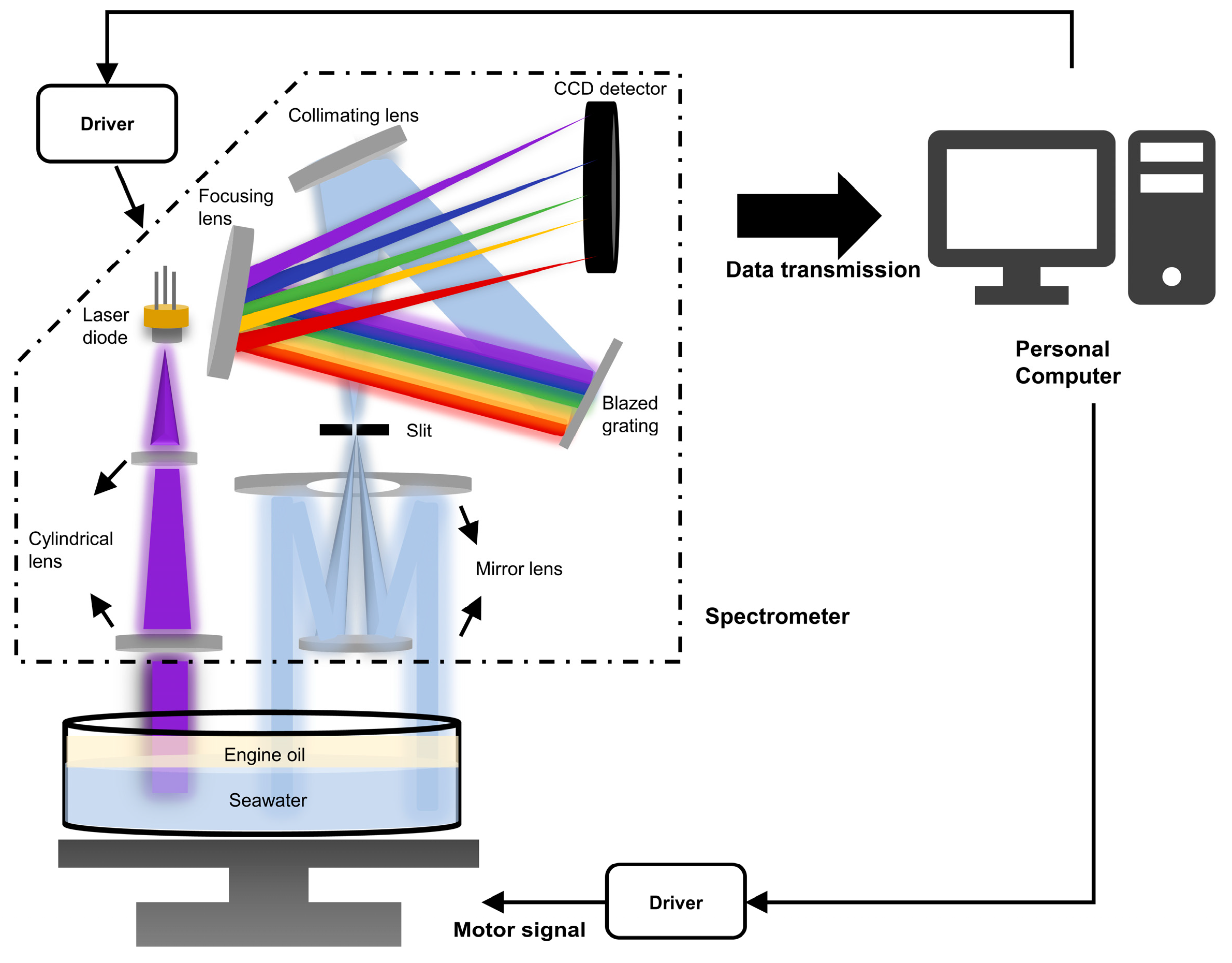
2.1. Experimental Scheme and Data Acquisition

The fluorescence spectra of five engine oils were collected under laboratory conditions. The samples included Shell HELIX 0W-40, Shell HELIX 5W-20, Mobil Super 4T 20W-50, Mobil Super 1000 X1 Diesel 15W-40, and Mobil 2000 5W-40. These petroleum products differ in application, viscosity, and chemical composition, leading to variations in their fluorescence spectra, including differences in intensity and characteristic peaks. The experiment involved placing equal amounts of seawater collected from the Yellow Sea of China (coordinates: 120.18° E, 35.82° N) into a Petri dish that was 7 cm in diameter. Oil samples were added in volumes of 0.2 mL, 0.4 mL, 0.6 mL, 0.8 mL, 1 mL, 1.5 mL, and 2 mL. After the oil spread into a uniform film, measurements were conducted using a self-developed portable spectrometer.

The experimental setup consisted of three components: a custom-built portable spectrometer with integrated transmission and reception systems, a six-axis motorized stage, and a personal computer. A schematic of the system is shown in Figure 1. The system comprises a transmission system, a reception system, and a dispersion system. The following describes the instrument components and signal acquisition process.

The laser source uses a 405 nm laser diode from Thorlabs (Newton, NJ, USA), delivering an adjustable power output from 1 to 100 mW. The emitted beam passes through a transmission system composed of two cylindrical mirrors that shape the divergence angle, ensuring uniform energy distribution over long distances. After collimation, the divergence angles are reduced from 78.5 mrad and 174.5 mrad to 1.8 mrad and 3 mrad, respectively, resulting in a focal spot of approximately 72 μm × 120 μm. At 60 mW of power, the beam achieves a power density of 0.885 MW/cm². The shaped beam is then directed perpendicularly onto an oil film floating on seawater. Upon receiving the laser energy, the fluorescent molecules in the oil absorb the energy, become excited, and subsequently emit fluorescence via spontaneous radiation. The reception system employs a custom-designed Cassegrain telescope with two parabolic mirrors. Featuring a primary mirror diameter of 95 mm and an effective focal length of 255 mm, the telescope efficiently collects fluorescence from the target area. It focuses the collected light onto a 35 μm-wide slit and directs the signal into the dispersion system. The dispersion system uses a crossed Czerny–Turner optical path to disperse the fluorescence signal. A reflective blaze grating with 600 lines/mm and a blaze angle of 8.6° is used; at 500 nm, the grating achieves a blaze efficiency of 68%, meeting the application requirements. The dispersed spectral signal is then focused by a lens onto Hamamatsu TDI-CCD image sensors, known for their high sensitivity and low noise performance, which enables the precise capturing of spectral variations. A control module synchronizes the laser driver and CCD timing, allowing the CCD to perform two measurements within a single laser cycle for background correction. Each spectrometer scan takes approximately 500 milliseconds and covers a spectral range of 400–750 nm.

To improve dataset diversity and reliability while better simulating real-world conditions, spectral data were collected for oil films of varying thicknesses at three laser power settings (60 mW, 70 mW, and 80 mW), with 30 samples recorded per power level. The spectrometer scan time was set to 5 s. The container holding the oil film and seawater was mounted on a six-axis motorized stage, which was programmed via control software to execute horizontal and vertical reciprocating motions over a 2 cm range, along with a simple harmonic tilting motion to simulate wave action. Additionally, to evaluate the effects of oil film thickness and laser power on fluorescence spectra, the pure fluorescence spectra of several engine oils were also collected.

2.2. Spectra Preprocessing and Augmentation Methods

Before training the model, we first used interpolations to remove the backscattering peak of the 405 nm laser observed during testing. Traditional oil film thickness measurement methods rely on fluorescence intensity and thus require calibration before measurements. However, in real-world environments, wind and waves cause fluctuations in fluorescence intensity that can generate false signals and degrade the accuracy of thickness inversion models. To mitigate this interference, we applied min–max normalization to scale the fluorescence spectra of oil films with different thicknesses to the [0, 1] range, enabling the model to focus on differences in spectral distribution related to film thickness.

Furthermore, spectral acquisition in practical settings is often affected by environmental and instrumental errors, which introduce noise and interference [38]. Traditional chemometric methods require preprocessing steps, such as noise removal, to improve the signal-to-noise ratio. In this study, to demonstrate the adaptive noise handling capabilities of our proposed framework, we evaluated the performance of the multi-task framework, traditional deep learning models, and chemometric models under various conditions: without preprocessing, with Savitzky–Golay (SG) filtering [39], standard normal variates (SNVs) [40], and normalization. The classification and regression results were statistically analyzed.

Traditional deep learning methods often require large datasets to learn feature relationships. Since there are no publicly available datasets for oil spill spectra and the collected data are limited, data augmentation is necessary to simulate real variations in spectral data. This helps improve model generalization under different operational conditions. In this study, we applied multiplication, noise addition, and random shift transformations to augment the dataset. The original dataset was split into training, validation, and test sets at a ratio of 3:1:1. Data augmentation was performed on the training set. Multiplication was adjusted using ±0.1 times the standard deviation of the training set, simulating variations in spectral intensity caused by sensor sensitivity and baseline shifts. Noise addition ranged from 1% to 5% of the training set’s standard deviation, mimicking spectral variations due to environmental light and instrument noise in real scenarios. Random shifts, limited to within 5 nm, were applied to simulate wavelength calibration differences between instruments. These shifts enhance model adaptability to various spectrometers, as calibration methods may cause slight wavelength offsets in measured spectra. For each spectral sample, the augmentation process was repeated nine times, increasing the dataset size from the original 4200 samples to 26,880.

2.3. Multi-Task Spectral Analysis Framework

The proposed network demonstrates a robust and efficient model for oil spill identification and thickness prediction, as illustrated in Figure 2. The Wavelet Transform CNN (WaveConv) block is used for multi-scale feature extraction from spectral data, reducing model parameters and improving computational efficiency. The scalar Long Short-Term Memory (sLSTM) block captures sequential dependencies, enhancing the model’s understanding of spectral feature positions. The Kolmogorov–Arnold Network-Enhanced Transformer (KET) block captures global data relationships, improving the model’s nonlinear representation capability. By integrating the WaveConv block, sLSTM block, and KET block, the model effectively captures both local and global spectral features. Moreover, the regression and classification tasks are seamlessly integrated into the core structure of the model. Instead of using separate fully connected layers, the features output by the KET block are directly mapped linearly to the classification and regression outputs. This design ensures that the core feature extraction modules also serve as predictive components, eliminating the need for additional fully connected layers while maintaining efficiency and simplicity.

2.3.1. Wavelet Transform CNN Block

The WaveConv block, shown in Figure 3a, is a critical component for lightweight network design and multi-scale feature extraction from spectral data. It consists of a CNN module and a Wavelet CNN module. Traditional CNN models for spectral analysis typically include multiple convolutional layers and fully connected layers. Convolutional layers are used for feature extraction and dimensionality reduction (e.g., through convolutional layers with large kernel sizes and strides), while fully connected layers combine extracted feature maps nonlinearly to enhance predictive capability. However, fully connected layers introduce a large number of parameters, reducing computational efficiency and increasing the risk of overfitting. In our previous research, we proposed a lightweight spectral analysis model that replaces fully connected layers with Global Average Pooling (GAP), reducing parameter counts while maintaining prediction accuracy [12]. Thus, the CNN module in the WaveConv block incorporates the core design from this model, as illustrated in Figure 3b. The CNN module includes three convolutional layers with residual connections to improve stability. Each convolution performs the following operation:

$$\begin{array}{c}y=\mathrm{ReLU}\left(\mathrm{B}\mathrm{N}\left(\mathrm{Conv}1\mathrm{d}\left(\mathrm{BN}\right(\mathrm{Conv}1\mathrm{d}(x\left)\right))\right)+\mathrm{S}\mathrm{h}\mathrm{o}\mathrm{r}\mathrm{t}\mathrm{c}\mathrm{u}\mathrm{t}\left(x\right)\right)\end{array}$$

(1)

where BN represents Batch Normalization, ReLU is the Rectified Linear Unit, and Shortcut denotes dimension-matched skip connections. After convolution, GAP compresses the feature dimensions to 1, and the features are flattened as the following:

$$\begin{array}{c}{z}_{\mathrm{cnn}}=\mathrm{F}\mathrm{l}\mathrm{a}\mathrm{t}\mathrm{t}\mathrm{e}\mathrm{n}\left(\mathrm{AdaptiveMaxPool}1\mathrm{d}\left(y\right)\right)\end{array}$$

(2)

However, CNNs can only extract local features, ignoring the sequential continuity of spectral data. For spectral analysis tasks, enhancing the model’s ability to understand feature sequences improves robustness and aligns with physical logic. Therefore, we introduced the Wavelet Transform Convolution (WTConv) operation to enhance the model’s multi-scale feature extraction capability.

Finder et al. [41] proposed an improved convolution operation, called Wavelet Transform Convolutions (WTConv), which increases the receptive field of the model without adding computational overhead. WTConv uses wavelet transforms to decompose features into high-frequency and low-frequency components, allowing convolution operations to focus on distinct frequency bands. Its effectiveness has been validated in image segmentation tasks. Inspired by WTConv, we simplified this into a Wavelet CNN module suitable for 1D data to extract multi-scale features, as illustrated in Figure 3c. The Wavelet CNN module operates as follows: First, a predefined wavelet filter (f_wavelet) is applied to the input tensor X∈ℝ^B×C×L (where B is the batch size, C is the number of channels, and L is the sequence length). The wavelet transform decomposes $X$ into W∈ℝ^B×C×2×L/2, containing low-frequency and high-frequency (W_LL and W_LH) components, as shown in Equation (3). Similarly, f_wavelet contains two filters: a low-pass filter and a high-pass filter (f_LL and f_LH).

$$\begin{array}{c}\mathrm{W}=\mathrm{WT}\left(X\right)=\mathrm{Conv1d}\left(X,{\mathrm{f}}_{\mathrm{w}\mathrm{a}\mathrm{v}\mathrm{e}\mathrm{l}\mathrm{e}\mathrm{t}},\mathrm{s}\mathrm{t}\mathrm{r}\mathrm{i}\mathrm{d}\mathrm{e}=2,\mathrm{p}\mathrm{a}\mathrm{d}\mathrm{d}\mathrm{i}\mathrm{n}\mathrm{g}=\mathrm{p}\mathrm{a}\mathrm{d}\right)\end{array}$$

(3)

After decomposition, convolutions are independently applied to the frequency components. For each decomposition level $\mathrm{i}$, the low-frequency (${\mathrm{W}}_{\mathrm{LL}}$) and high-frequency (${\mathrm{W}}_{\mathrm{LH}}$) components are processed using small 1D convolutional kernels (${\mathrm{W}}_{\mathrm{c}\mathrm{o}\mathrm{n}\mathrm{v}}$):

$$\begin{array}{c}{\mathrm{Y}}_{\mathrm{L}\mathrm{L}}^{\left(\mathrm{i}\right)},{\mathrm{Y}}_{\mathrm{L}\mathrm{H}}^{\left(\mathrm{i}\right)}=\mathrm{ReLU}\left(\mathrm{C}\mathrm{o}\mathrm{n}\mathrm{v}1\mathrm{d}\left(\left[{\mathrm{W}}_{\mathrm{L}\mathrm{L}}^{\left(\mathrm{i}\right)},{\mathrm{W}}_{\mathrm{L}\mathrm{H}}^{\left(\mathrm{i}\right)}\right],{\mathrm{W}}_{\mathrm{c}\mathrm{o}\mathrm{n}\mathrm{v}}\right)\right)\end{array}$$

(4)

After convolution, the wavelet components are reconstructed back into the spatial domain using the inverse wavelet transform:

$$\begin{array}{c}\mathrm{Z}=\mathrm{IWT}\left({\mathrm{Y}}_{\mathrm{L}\mathrm{L}},{\mathrm{Y}}_{\mathrm{L}\mathrm{H}}\right)=\mathrm{ConvTranspose1d}\left(\mathrm{Y},{\mathrm{f}}_{\mathrm{w}\mathrm{a}\mathrm{v}\mathrm{e}\mathrm{l}\mathrm{e}\mathrm{t}}^{\mathrm{\top }},\mathrm{s}\mathrm{t}\mathrm{r}\mathrm{i}\mathrm{d}\mathrm{e}=2,\mathrm{p}\mathrm{a}\mathrm{d}\mathrm{d}\mathrm{i}\mathrm{n}\mathrm{g}=\mathrm{p}\mathrm{a}\mathrm{d}\right)\end{array}$$

(5)

Here, ${\mathrm{f}}_{\mathrm{w}\mathrm{a}\mathrm{v}\mathrm{e}\mathrm{l}\mathrm{e}\mathrm{t}}^{\mathrm{\top }}$ represents the reconstruction filters, and Z ∈ ℝ^B×C×L is the reconstructed feature map. The final output of the Wavelet CNN module is expressed in Equation (6), where ${\mathrm{X}}_{\mathrm{b}\mathrm{a}\mathrm{s}\mathrm{e}}$ represents the base convolution operation, and ${\mathrm{Z}}_{\mathrm{w}\mathrm{a}\mathrm{v}\mathrm{e}\mathrm{l}\mathrm{e}\mathrm{t}}$ is the reconstructed wavelet output:

$$\begin{array}{c}Z={\mathrm{X}}_{\mathrm{b}\mathrm{a}\mathrm{s}\mathrm{e}}+{\mathrm{Z}}_{\mathrm{w}\mathrm{a}\mathrm{v}\mathrm{e}\mathrm{l}\mathrm{e}\mathrm{t}}\end{array}$$

(6)

In the WaveConv block, spectral data are passed through both the CNN–Wavelet CNN module and the Wavelet CNN module independently, with the output features combined at the end. This design enhances the feature extraction capabilities of the WaveConv block by effectively integrating local focus regions with multi-scale feature information. Additionally, the incorporation of wavelet transforms improves the model’s noise resistance.

2.3.2. Scalar Long Short-Term Memory Block

Considering the inherent continuity of spectral features, traditional convolution-based feature extraction methods struggle to establish feature correlations. To address this, we use the scalar Long Short-Term Memory (sLSTM) method to learn the sequential dependencies in the feature output by the WaveConv block. sLSTM enhances traditional LSTMs by introducing an exponential gate in the input and forget gates to replace the sigmoid function used in conventional LSTMs. Additionally, a new memory mixing mechanism is incorporated [42]. These modifications improve the stability of sLSTM when handling long sequences, making it particularly suitable for tasks such as time-series prediction and natural language processing. Figure 4 illustrates the computational process of the sLSTM block as well as the detailed calculation steps within a single sLSTM module. The sLSTM block contains multiple sLSTM modules, with green and orange arrows representing bidirectional information transmission.

2.3.3. Kolmogorov–Arnold Network-Enhanced Transformer Block

The transformer architecture, first introduced by Vaswani et al. [43], has revolutionized natural language processing due to its outstanding attention mechanism and position-encoding methods. It has since been widely adopted in fields such as computer vision, time-series analysis, and spectral data classification. However, transformers have certain limitations. The feedforward layers in traditional transformers consist of multiple fully connected layers, which are the main contributors to the model’s parameters. This increases computational complexity and memory requirements, making transformer-based oil spill analysis models challenging to deploy on resource-constrained hardware. Moreover, the simplistic linear transformations and activation functions in the feedforward layers struggle to model the highly nonlinear relationships in spectral data, while dense parameterization increases the risk of overfitting.

To address these issues and enable the model to focus on different parts of the oil spill spectra simultaneously—capturing both local and global dependencies—we propose an improved transformer structure. Kolmogorov–Arnold Networks (KANs) replace the feedforward layers in the original transformer, eliminating the need for fully connected layers. Additionally, the multi-head attention mechanism is enhanced by applying KAN-based nonlinear mapping to its output, reducing the parameter count while improving nonlinear representation capabilities. This module, referred to as the Kolmogorov–Arnold Network-Enhanced Transformer (KET) block, is illustrated in Figure 5a.

KAN, introduced by Liu et al. [44], leverages learnable activation functions on edges to replace traditional linear weights. This novel architecture enhances model expressiveness and interpretability, particularly for compositional tasks. The computational process of the KAN module is shown in Figure 5b. Each learnable edge function (${\varphi }_{j,i}$) combines a base activation function (b(x)) and a spline (s(x)), defined as follows:

$$\begin{array}{c}{\varphi }_{j,i}\left(x\right)=w\cdot \left(b\left(x\right)+s\left(x\right)\right)\end{array}$$

(7)

where $b\left(x\right)=silu\left(x\right)$ and $s\left(x\right)={\sum }_k{c}_k{B}_k\left(x\right)$, with $B_k\left(x\right)$ being B-spline basis functions. In the proposed KET block, each linear transformation in the original feedforward layer is replaced by the following:

$$\begin{array}{c}{f}_{KAN}\left(x\right)={\mathsf{\Phi }}_2\left({\mathsf{\Phi }}_1\left(x\right)\right)\end{array}$$

(8)

where ${\mathsf{\Phi }}_1$ and ${\mathsf{\Phi }}_2$ are KAN layers with learnable spline-based edge functions.

Additionally, the attention mechanism output in the transformer is passed through KAN-based nonlinear mapping:

$$\begin{array}{c}\mathrm{KAN}\left(\mathrm{Q},\mathrm{K},\mathrm{V}\right)={\mathsf{\Phi }}_{KAN}\left(\mathrm{ATTENTION}\left(Q,K,V\right)\right)\end{array}$$

(9)

This ensures that the model effectively captures complex compositional structures and single-variable feature intricacies. By replacing the original dense layers with KAN, the KET block achieves a more compact representation, reducing the parameter count while maintaining performance. With the incorporation of KAN’s learnable nonlinear mapping capabilities, the KET block captures complex spectral features and relationships that are often overlooked by traditional dense layers. Furthermore, KAN’s reduced sensitivity to noise makes the enhanced transformer module more robust when handling real-world spectral data. The lower parameter count also makes the spectral analysis framework more suitable for deployment on resource-constrained devices, enabling real-time oil spill spectral analysis.

2.3.4. Training Parameters and Strategy

The model was trained using the Adam optimizer, which adaptively adjusts learning rates for each parameter based on the first moment (mean) and second moment (uncentered variance) of the gradients during optimization [45]. For the loss functions, cross-entropy loss was used to evaluate the classification performance, while mean-square-error (MSE) loss was used to assess regression predictions. Other hyperparameters of the model were optimized using the Bayesian Optimization (BO) method with the ‘Optuna’ package (3.6.1) to identify the optimal values. The results of the hyperparameter optimization are shown in

Table 1. Hyperparameter optimization results.

Hyperparameter	Range/Values	Optimal Solution
Learning rate	[1 × 10−5, 1 × 10−3]	6.922 × 10−5
Batch size	[32, 64, 128, 256, 512]	32
Kernel sizes	[3, 19]	[19, 5, 17]
Strides	[1, 5]	[3, 5, 5]
Number of layers (LSTMs)	[2, 5]	3
Transformer dropout rate	[0.1, 0.5]	0.5
Transformer blocks	[2, 5]	4
Attention heads	[2, 4, 8, 16]	4
Embedding dimension	[64, 128, 256, 512]	64
Dense dimension	[64, 128, 256, 512]	256

. An early stopping mechanism was introduced to monitor the training process, halting training if the validation loss did not decrease after 10 epochs. The final number of training epochs was set to 400. The training was performed on an NVIDIA GTX-3090 GPU with CUDA 11.8 and cuDNN 8.7.0 environments. The implementation of the proposed method was programmed using PyTorch 2.0.0 in a Python 3.10.10 environment.

2.4. Model Evaluation Methods

2.4.1. Evaluation Metrics

This study employs various metrics to comprehensively evaluate the classification and regression performance of the model. For the classification task, a confusion matrix, accuracy, macro-precision, macro-recall, and the macro-F1 score were used as evaluation metrics. The confusion matrix visually presents prediction results, while accuracy measures the overall correctness of the model’s predictions. Meanwhile, precision evaluates the proportion of correctly predicted positive samples among all predicted positives, and recall measures the proportion of actual positives correctly identified. The F1 score, the harmonic mean of precision and recall, balances these two metrics.

In our multi-class setting, we adopt macro averaging for precision, recall, and the F1 score: we first compute these metrics for each class independently, then take the unweighted mean across all classes, giving each class equal importance. The formulas for these metrics (in their classic binary form) are provided in Equations (10)–(13), where $TP$, $TN$, $FP$, and $FN$ represent true positives, true negatives, false positives, and false negatives, respectively:

$$\begin{array}{c}\mathrm{Accuracy}={\displaystyle \frac{TP+TN}{TP+TN+FP+FN}}\end{array}$$

(10)

$$\begin{array}{c}\mathrm{Precision}={\displaystyle \frac{TP}{TP+FP}}\end{array}$$

(11)

$$\begin{array}{c}\mathrm{Recall}={\displaystyle \frac{TP}{TP+FN}}\end{array}$$

(12)

$$\begin{array}{c}\mathrm{F}1-\mathrm{S}\mathrm{c}\mathrm{o}\mathrm{r}\mathrm{e}={\displaystyle \frac{2·\mathrm{Precision}·\mathrm{Recall}}{\mathrm{Precision}+\mathrm{Recall}}}\end{array}$$

(13)

For the regression task, the key evaluation metrics include the coefficient of determination ($R^2$), mean absolute error (MAE), root-mean-square error (RMSE), and Residual Predictive Deviation (RPD). These metrics are calculated using Equations (14)–(17):

$$\begin{array}{c}{R}^2=1-{\displaystyle \frac{{\sum }_{i=1}^n{\left(y_i-{\widehat{y}}_i\right)}^2}{{{(y}_i-\overline{y})}^2}}\end{array}$$

(14)

$$\begin{array}{c}\mathrm{M}\mathrm{A}\mathrm{E}={\displaystyle \frac{1}{n}}{\displaystyle \sum _{i=1}^n}\left|y_i-{\widehat{y}}_i\right|\end{array}$$

(15)

$$\begin{array}{c}\mathrm{R}\mathrm{M}\mathrm{S}\mathrm{E}=\sqrt{{\displaystyle \frac{1}{n}}{\displaystyle \sum _{i=1}^n}{\left(y_i-{\widehat{y}}_i\right)}^2}\end{array}$$

(16)

$$\begin{array}{c}\mathrm{RPD}={\displaystyle \frac{{\sigma }_y}{RMSE}}\end{array}$$

(17)

Here, $y_i$ is the actual value, ${\widehat{y}}_i$ is the predicted value, $\overline{y}$ is the mean of the actual values, and ${\sigma }_y$ is the standard deviation of the actual values. $R^2$ measures the proportion of variance in the target variable explained by the model inputs; values closer to 1 indicate better predictive performance. MAE quantifies the average magnitude of prediction errors, offering an intuitive measure of accuracy. RMSE calculates the square root of the average squared differences between predicted and actual values, highlighting the model’s ability to minimize large prediction errors. RPD evaluates the ratio of the standard deviation of actual values to the model’s RMSE, reflecting the model’s predictive reliability. A higher RPD indicates better generalization capabilities and performance on diverse data distributions.

2.4.2. Model Comparison

To demonstrate the advantages of the proposed Hybrid framework, we conducted comparative experiments for classification and regression tasks. For classification, the framework was compared with SVM, KNN, and a traditional transformer model. For regression, comparisons were made with SVM, LR, and the transformer model. A grid search combined with 5-fold cross-validation was used to optimize the hyperparameters of the SVM, KNN, and LR models. During each cross-validation, the performance on the validation set was used to evaluate the parameter settings and determine the final values. For the transformer model, it was also designed as a unified framework for simultaneous classification and regression tasks, and its hyperparameters were extensively optimized using the Bayesian Optimization (BO) method. Both the raw dataset (without preprocessing) and the preprocessed dataset were used to train the above models. The classification and regression performances of the models were analyzed and compared.

3. Results and Discussion

3.1. Spectral Analysis

Figure 6 presents the fluorescence spectra of five oils measured at the laser powers of 60 mW, 70 mW, and 80 mW. Solid lines indicate the average spectra, while shaded areas represent spectral variability under specific film thickness and laser power conditions. The spectra reveal similar features across the oils, with prominent peaks around 490 nm and 530 nm. A peak near 470 nm corresponds to the Raman signal of seawater, and a peak near 610 nm likely originates from organic matter in the seawater. These findings are consistent with those reported by Zhang et al. [26]. As laser power increases, the fluorescence intensity of the oils also increases. For example, Figure 6a–c demonstrate that the fluorescence spectra of Shell HELIX 0W-40 tend to saturate at 80 mW, leading to a diminution of the two primary peaks. In contrast, the other oils do not exhibit noticeable saturation at a high laser power, indicating that intrinsic differences among oils result in varied laser responses. Additionally, as oil film thickness increases, the seawater Raman peak diminishes; however, the degree of attenuation varies among different oils. Even for the same oil, the intensity variation of the Raman peak differs under different laser powers. These observations suggest that differences in the optical absorption properties of each oil affect the suppression of the seawater Raman signal. Consequently, traditional oil film thickness estimation methods, such as Raman suppression techniques, often require adjusting model parameters based on oil type and laser power, increasing workflow complexity and reducing model practicality. Moreover, the predictive thickness range varies among different oils, which severely limits the generalizability of these methods. Furthermore, since spectral acquisition occurs during dynamic processes, the relative position of the oil film and detector (horizontal and vertical distances, as well as angles) is constantly changing. For oil films with similar thicknesses, the spectral intensity may overlap. Existing thickness prediction methods rely on static data collected in laboratories to fit models. However, significant spectral variations in real-world environments can lead to model failure. The relationship between oil thickness and fluorescence intensity in Figure 6 is nonlinear for different oils. Even for the same oil, due to the simulated wave action, the transformation between thickness and fluorescence intensity is inconsistent under different laser powers (e.g., Figure 6j–l).

Figure 7 illustrates the fitting relationship between fluorescence intensity and oil film thickness for Helix 0W-40 and Mobil 2000 5W-40 under static conditions at three different laser power levels. This figure shows that fluorescence intensity increases with oil film thickness, exhibiting an exponential-like trend. A cubic polynomial model was used to effectively capture this nonlinear relationship. Moreover, due to inherent differences in light absorption, the thickness–intensity relationship varies among oils, as evidenced by the distinct fitted curves for Helix 0W-40 and Mobil 2000 5W-40. This phenomenon indicates that oil type and film thickness are interrelated and must be analyzed comprehensively.

To illustrate the effects of oil type and film thickness on spectral distribution, pure oil spectra were collected for 100 mL samples of five different engine oils, as shown in Figure 8. A comparison revealed differences in both spectral features and distribution between the pure oil spectra and the spectra of oil films with varying thicknesses. For example, the pure oil spectrum of Mobil Super 1000 X1 Diesel 15W-40 shows two prominent fluorescence peaks near 490 nm and 530 nm, with an intensity ratio close to 1:1. However, as Figure 6j–l demonstrates, the spectral profile of Mobil Super 1000 X1 Diesel 15W-40 initially resembles that of the pure oil when the film is thin but changes as the film thickens. This behavior is likely due to interfacial effects between the oil and seawater, which influence the fluorescence characteristics as well as light propagation effects in the oil film and seawater. These findings indicate that the quantity of spilled oil alters the fluorescence spectral distribution. Therefore, oil-type identification and oil film thickness prediction should be analyzed concurrently to capture their synergistic effects. Separating these tasks with traditional methods may undermine the practical utility of LIF technology in field applications.

The spectral acquisition results further indicate that the oil type, detection mode, and laser power significantly influence the fluorescence spectra of oil spills. Traditional methods often overlook the interrelations among these factors, raising concerns about their accuracy and practicality. In contrast, our data acquisition system effectively simulates real-world oil spill scenarios. Combined with a multi-task deep learning framework that simultaneously predicts oil type and film thickness, the system enhances the model’s comprehensiveness, practicality, and reliability.

3.2. Model Training Process

Figure 9 depicts the training progress of the Hybrid framework and the transformer model. With the combination of Bayesian Optimization (BO) and early stopping, the number of training epochs for the transformer model was set to 1000. From the loss convergence curves of the two models, it can be observed that the proposed framework converges faster, with the loss dropping below 0.1 at around 30 epochs and stabilizing after 300 epochs. In contrast, the transformer model reaches a loss of 0.1 only after approximately 250 epochs and stabilizes at around 700 epochs. Additionally, the proposed framework demonstrates better stability during training, with a smooth loss curve and minimal spikes. In contrast, the transformer model exhibits numerous spikes in the early training phase, likely due to the large number of parameters in its feedforward layers and the simplicity of its linear transformations, which make it prone to gradient vanishing when handling long sequences. Furthermore, the high complexity of the fluorescence dataset and the introduction of noisy data through augmentation exacerbate the transformer’s sensitivity to noise, leading to model degradation during training.

3.3. Model Performance Evaluation

3.3.1. Classification Performance

After training, we saved the model that performed best on the validation set and evaluated its performance on the test set using classification metrics. The performance of the proposed framework was compared with that of traditional transformer, SVM, and KNN models. Figure 10 presents the confusion matrices for the four models on the test set without data preprocessing. As shown in Figure 10a, the proposed framework achieved the best classification performance, with only two misclassified samples, where two Mobil 2000 5W-40 samples were misclassified as Mobil Super 4T 20W-50. From the spectral graphs in Figure 6, it is evident that these two oils have similar spectra, and the dynamic measurement process introduces fluctuations in spectral intensity. Therefore, we consider this misclassification within the acceptable error range of the model. Similarly, the transformer model also demonstrated a classification performance comparable to the Hybrid framework. Considering the complexity of the fluorescence dataset, especially in terms of thickness variations, and the similarity between oil spectra, it is reasonable that the transformer model, which has been well-validated in large-scale language tasks, performs similarly to the proposed model. In contrast, the SVM and KNN models performed significantly worse than the deep learning models on the unprocessed dataset. Both SVM and KNN exhibited notable errors in identifying Mobil Super 4T 20W-50 and Mobil 2000 5W-40 samples. This indicates that traditional machine learning models struggle to accurately identify spectral features in the presence of complex interference signals.

Next, the balance of the models’ performance on the training and test sets was examined. As shown in

Table 2. Classification evaluation index results of the model.

Model	Accuracy (Train)	Recall (Train)	Precision (Train)	F1 Score (Train)	Accuracy (Test)	Recall (Test)	Precision (Test)	F1 Score (Test)
Hybrid framework	99.98%	99.99%	99.98%	0.9998	99.76%	99.76%	99.73%	0.9975
Transformer	99.96%	99.97%	99.97%	0.9997	99.52%	99.53%	99.5%	0.9951
SVM	89.83%	89.82%	89.85%	0.8972	92.62%	92.16%	92.42%	0.9223
KNN	87.52%	87.46%	88.56%	0.8733	93.81%	93.68%	94.08%	0.9351

, the two deep learning-based models performed similarly, with the proposed Hybrid framework achieving slightly better results. For SVM and KNN, their classification performance on the test set was better than on the training set. This may be due to the broader distribution and higher complexity of the augmented training data compared to the test set. As a result, even though these models struggled with the training set, the learned distributions aligned more closely with the test set. This outcome further demonstrates the effectiveness of the data augmentation method.

For traditional spectral analysis methods, data preprocessing is necessary to filter out interference signals. However, different preprocessing methods affect model performance in various ways, making preprocessing an additional hyperparameter for oil spill spectral analysis models. If a model can filter out interference signals during feature extraction without relying on preprocessing, it would have faster response times and greater practicality.

Table 3. Test set classification evaluation index results.

Methods	Raw		SG		SG + SNV		Normalization
Hybrid Framework	Accuracy	99.76%	Accuracy	99.82%	Accuracy	99.76%	Accuracy	99.82%
	Recall	99.76%	Recall	99.81%	Recall	99.75%	Recall	99.81%
	Precision	99.73%	Precision	99.79%	Precision	99.74%	Precision	99.79%
	F1 score	0.9975	F1 score	0.9980	F1 score	0.9974	F1 score	0.9980
Transformer	Accuracy	99.52%	Accuracy	99.88%	Accuracy	99.52%	Accuracy	99.88%
	Recall	99.53%	Recall	99.88%	Recall	99.53%	Recall	99.88%
	Precision	99.50%	Precision	99.87%	Precision	99.52%	Precision	99.87%
	F1 score	0.9951	F1 score	0.9987	F1 score	0.9952	F1 score	0.9987
SVC	Accuracy	92.62%	Accuracy	92.5%	Accuracy	97.26%	Accuracy	92.74%
	Recall	92.16%	Recall	92.02%	Recall	97.13%	Recall	92.31%
	Precision	92.42%	Precision	92.32%	Precision	97.10%	Precision	92.60%
	F1 score	0.9223	F1 score	0.9210	F1 score	0.9711	F1 score	0.9237
KNN	Accuracy	93.81%	Accuracy	93.93%	Accuracy	93.69%	Accuracy	93.81%
	Recall	93.68%	Recall	93.82%	Recall	93.46%	Recall	93.68%
	Precision	94.08%	Precision	94.09%	Precision	93.75%	Precision	93.93%
	F1 score	0.9351	F1 score	0.9363	F1 score	0.9342	F1 score	0.9351

shows the classification performance of four models on the test set under no preprocessing and three preprocessing combinations.

As shown in Table 3, the proposed Hybrid framework demonstrates consistent performance across different preprocessing methods, while the transformer model significantly improves its classification performance after SG filtering and normalization. This aligns with the transformer’s sensitivity to noise. After SG filtering, noise in the spectra is significantly reduced, resulting in improved transformer performance. In contrast, the proposed Hybrid framework, due to the effective integration of the WaveConv block, sLSTM block, and KET block, exhibits reduced sensitivity to external interference and enhanced feature extraction and recognition capabilities. For KNN and SVM, their performance fluctuates under different preprocessing methods, further demonstrating the uncertain impact of preprocessing on spectral models. The proposed framework achieves better classification performance than traditional methods and classic deep learning models even without preprocessing. Its robustness to noise makes it well-suited for fast oil spill spectral analysis in complex environments.

3.3.2. Regression Performance

As shown in Figure 6, the relationship between oil film thickness and fluorescence intensity varies across different oil types under different laser powers. Combined with the simulated wave environment used in our experiments, the data exhibit high nonlinearity.

Table 4. The thickness prediction performance of the model.

Model	MAE	RMSE	R2	RPD
Hybrid framework	0.0068	0.0212	0.9806	7.1876
Transformer	0.0266	0.0375	0.9392	4.0542
SVM	0.4000	0.5420	0.7028	1.8343
LR	0.5446	0.6639	0.5541	1.4976

summarizes the regression performance of the four models on the test set.

From Table 4, it is evident that the proposed Hybrid framework significantly outperforms the other methods in thickness prediction. The test set’s R² value being close to 1 indicates a strong correlation between predicted and actual values, demonstrating that the model has effectively learned and can generalize to a broader data range. The lower RMSE suggests that the proposed method has the smallest prediction error for oil film thickness compared to other models. The RPD value of 7.1876 for the Hybrid framework indicates exceptional robustness and stability. An RPD greater than 2 generally signifies a good predictive ability for most applications, while an RPD above 5 indicates a highly reliable model. The transformer model has an RMSE close to that of the Hybrid framework, but its R² and RPD values are significantly lower. This suggests that although the transformer can predict thickness to some extent, it lacks extrapolation capabilities and struggles with unseen data. This limitation stems from its feedforward layers, which rely on simple linear transformations. In contrast, the KET module in the proposed framework leverages the nonlinear mapping power of KAN, resulting in predictions that closely correlate with actual values and generalize effectively to other thickness ranges. Traditional regression models like SVM and LR exhibit poor performance on the highly nonlinear fluorescence dataset due to their limited nonlinear modeling capabilities. As a result, they are unable to effectively predict oil film thickness.

It is worth noting that our oil film thickness range spans from 50 µm to 0.5 mm, covering both thin and thick films, with broad sample diversity. The evaluation metrics in Table 4 reflect the model’s overall performance rather than its performance for individual oil types. Previous analyses of oil spill spectra revealed that the Raman peak intensity, fluorescence spectral features, and thickness at which Raman peaks disappear vary across oil types, influenced by laser power, wave effects, and intrinsic properties. Traditional methods like fluorescence and Raman suppression often fail to account for these additional factors, reducing their practicality and robustness. The proposed Hybrid framework, with its robust multi-scale feature extraction capabilities, achieves accurate predictions across a wide range of thicknesses and complex scenarios. This demonstrates the model’s excellent generalization and adaptability, making it suitable for real-world applications.

Figure 11 shows the scatter plots of predictions for the test set of five oils by the two deep learning models. From this figure, it is evident that both models perform differently for each oil type. The Hybrid framework performs best for Mobil Super 1000 X1 Diesel 15W-40, although there is greater prediction variance for the 0.39 mm oil film thickness. This is because at 60 mW laser power, the fluorescence intensity variation for this thickness differs from that under other power conditions, posing challenges for thickness prediction. For the proposed model, the RPD values for regression predictions across all oil types exceed 5, with R² values generally above 0.97, indicating a strong extrapolation ability and applicability to unseen data. In comparison, the transformer model’s RPD values are consistently below 5, with a lower RMSE and R², which aligns with its overall performance in Table 4. On the other hand, the results in Figure 11 highlight the importance of verifying the generalization capability of oil spill analysis models during development. Due to variations in intrinsic properties and external disturbances, thickness prediction performance may differ across oil types. This result further demonstrates that the proposed method is versatile, capable of learning individual spectral features for different oils. With continued data augmentation, the model has the potential to become a universal framework for oil spill thickness analysis.

Similar to Section 3.3.1,

Table 5. Test set regression evaluation index results.

Methods	Raw		SG		SG + SNV		Normalization
Hybrid Framework	MAE	0.0068	MAE	0.0090	MAE	0.0075	MAE	0.0076
	RMSE	0.0212	RMSE	0.0241	RMSE	0.0229	RMSE	0.0209
	R2	0.9806	R2	0.9750	R2	0.9774	R2	0.9810
	RPD	7.1876	RPD	6.3188	RPD	6.6544	RPD	7.2614
Transformer	MAE	0.0266	MAE	0.0250	MAE	0.0241	MAE	0.0251
	RMSE	0.0375	RMSE	0.0349	RMSE	0.0358	RMSE	0.0355
	R2	0.9392	R2	0.9473	R2	0.9446	R2	0.9455
	RPD	4.0542	RPD	4.3567	RPD	4.2505	RPD	4.2816
SVC	MAE	0.4000	MAE	0.4059	MAE	0.4264	MAE	0.4058
	RMSE	0.542	RMSE	0.5490	RMSE	0.5679	RMSE	0.5499
	R2	0.7028	R2	0.6962	R2	0.6737	R2	0.694
	RPD	1.8343	RPD	1.8109	RPD	1.7507	RPD	1.8079
LR	MAE	0.5446	MAE	0.5446	MAE	0.5498	MAE	0.5459
	RMSE	0.6639	RMSE	0.6639	RMSE	0.6754	RMSE	0.6661
	R2	0.5541	R2	0.5541	R2	0.5385	R2	0.5511
	RPD	1.4976	RPD	1.4976	RPD	1.472	RPD	1.4925

summarizes the regression performance of different methods under various preprocessing conditions. From Table 5, it can be observed that preprocessing does not significantly improve regression performance across the models. Instead, similar to the classification task, performance fluctuations are noted. Given the high complexity of the dataset, strong nonlinear capabilities are required, and preprocessing cannot enhance the nonlinearity of the models. The proposed Hybrid framework outperforms other models significantly, even without preprocessing. While slight performance fluctuations occur after SG and SNV preprocessing, the RMSE remains around 0.2, indicating that additional interference signals, introduced by preprocessing, do not cause significant prediction deviations. Moreover, the RPD and R² values remain high, confirming the model’s reliability. The transformer model shows an improvement in regression performance after preprocessing, suggesting that preprocessing reduces noise interference in the data, partially addressing the transformer’s sensitivity to noise. However, the performance gain is limited, which is related to the transformer’s constrained nonlinear mapping capability. This further highlights the necessity of improving the transformer model using the KAN method.

To account for the strong noise interference in marine environments, noise signals with SNR of 15 dB, 20 dB, 25 dB, and 30 dB were added to the dataset to evaluate the noise robustness of the proposed Hybrid framework.

Table 6. Results of robustness testing for Hybrid framework and transformer.

Model	SNR (dB)	Accuracy	Precision	Recall	F1 Score	MAE	RMSE	R2	RPD
Hybrid Framework	GT	0.9976	0.9973	0.9976	0.9975	0.0068	0.0212	0.9806	7.1876
	15	0.8357	0.8475	0.8397	0.8402	0.0365	0.0651	0.8166	2.3353
	20	0.9405	0.9427	0.9435	0.9428	0.0256	0.0489	0.8965	3.1079
	25	0.9786	0.9797	0.9801	0.9799	0.0161	0.0343	0.9492	4.4371
	30	0.9952	0.9949	0.9954	0.9951	0.0081	0.0234	0.9763	6.5
Transformer	GT	0.9952	0.995	0.9953	0.9951	0.0266	0.0375	0.9392	4.0542
	15	0.5488	0.5734	0.5472	0.5387	0.1105	0.1431	0.1141	1.0625
	20	0.7417	0.7544	0.7443	0.7409	0.0852	0.1144	0.4345	1.3298
	25	0.9202	0.9212	0.9225	0.9212	0.0567	0.0797	0.7251	1.9072
	30	0.9714	0.9721	0.9719	0.9719	0.0387	0.0541	0.8736	2.8124

summarizes the classification and regression performance of both the Hybrid framework and the transformer model under these different noise conditions. In classification tasks, as noise levels increase, the Hybrid framework demonstrates notable robustness. At an SNR of 15 dB, its accuracy is 0.8357, a reduction of only about 16% compared to the noise-free case. As noise decreases, the classification performance recovers rapidly; at 30 dB, the model achieves an accuracy of 0.9952, nearly identical to the noise-free scenario, indicating strong noise adaptability.

For regression tasks, the proposed model also exhibits strong resilience. Although at 15 dB, the MAE and RMSE increase significantly and regression performance degrades compared to the noise-free condition, the R² value remains above 0.8, and the RPD exceeds 2, indicating that the model’s regression predictions are still meaningfully correlated. As noise diminishes, the regression performance gradually recovers, reaching levels comparable to the noise-free state at 30 dB.

In contrast, the transformer model is severely affected by noise. In classification tasks at 15 dB, its accuracy drops sharply to 0.5488, a decline of roughly 41% compared to the noise-free condition. Its regression performance also deteriorates dramatically, with an R² of only 0.1141 and an RPD of 1.0625 at 15 dB, which is close to random prediction. This suggests that the transformer’s global attention weights are significantly disrupted by noise, impairing effective feature extraction.

Overall, these robustness tests indicate that the designed WaveConv block significantly enhances the model’s noise resilience. Its multi-scale convolutional kernels and residual connections create a synergistic path for local denoising and global fitting, achieving a balanced improvement in noise robustness and multi-task performance. This advancement further enhances the practicality of LIF technology.

Table 7. Performance of Hybrid framework and transformer.

Method	Accuracy	R2	RPD	Iteration	Noise Sensitivity	Parameter
Hybrid Framework	99.76%	0.9806	7.1876	400	16.48%	4.57 M
Transformer	99.52%	0.9392	4.0542	1000	66.34%	16.79 M

summarizes the key metrics, stable training epochs, noise sensitivity, and parameter counts for both the Hybrid framework and the transformer model. Here, noise sensitivity is defined as the average reduction in accuracy and R² at an SNR of 15 dB relative to the baseline. The results show that while both models perform similarly in classification tasks, the proposed framework significantly outperforms the transformer model in regression tasks. Owing to the multi-scale feature extraction capability of the WaveConv module and the nonlinear mapping ability of KAN, the Hybrid framework requires fewer training epochs and exhibits enhanced robustness. Additionally, the lightweight design of the WaveConv and KET block allows the framework to achieve high predictive performance without relying on fully connected layers. With only 4.57 M parameters, the framework is ideally suited for deployment on resource-constrained, miniaturized hardware systems.

Although the proposed Hybrid framework achieves simultaneous predictions for oil spill classification and regression tasks, it has certain limitations. The current validation primarily focused on distinguishing oil types, while other organic materials commonly coexisting in marine environments (e.g., natural dissolved organic matter, microplastics, and biological substances) were not systematically incorporated into the spectral dataset. This omission may challenge the framework’s discrimination accuracy in real-world scenarios, where complex material mixtures exist, as evidenced by recent LIF-based studies demonstrating the necessity of multi-material comparisons for robust identification [46]. Additionally, the model’s performance depends critically on the representativeness of input spectral data. Due to experimental constraints, training and validation were conducted using laboratory-collected data rather than field measurements from dynamic marine environments, potentially limiting practical applicability. Observed performance fluctuations during preprocessing stages further suggest that the model’s stability may be compromised when encountering severe noise interference or unexpected spectral artifacts in real-time detection.

Future work will focus on expanding the spectral database to encompass diverse marine organic materials and validating the model’s online analysis capability using more real-world data to enhance its practicality. Transfer learning strategies will be explored to improve the model’s adaptability, enabling broader applications in more complex and diverse spectral analysis tasks. Integrating the framework into an end-to-end online spectral detection system presents a promising direction for future research, with the potential to significantly enhance its applicability in industrial and field environments.

4. Conclusions

This article proposes a novel oil spill spectral analysis method that simultaneously identifies oil types and predicts oil film thickness. The method integrates a self-designed detection and environmental simulation system, which significantly improves the reliability of the dataset and the practicality of the model. Furthermore, the proposed lightweight multi-task unified framework, the Wavelet CNN-sLSTM-KET framework, demonstrates the ability to handle both classification and regression tasks using fluorescence spectra without relying on fully connected layers. The framework achieves high accuracy and robustness in classification tasks and effectively predicts oil film thicknesses across a range of 50 µm to 0.5 mm, achieving strong R² and RPD values and low RMSE values, all without requiring preprocessing. Moreover, thanks to its well-conceived architecture and innovative feature extraction modules, the model’s performance decreases by only 16% under high-noise conditions, indicating excellent robustness. These characteristics establish the proposed framework as a foundational solution for fast, general, and precise oil spill spectral analysis, driving advancements in non-destructive oil spill detection technologies. Its scalability, real-time capability, and lightweight design overcome the limitations of traditional oil spill analysis models, making it highly suitable for practical applications. Future research will aim to expand the representativeness of the dataset to further improve the model’s generalizability and robustness. The development of miniaturized spectrometer devices could broaden the framework’s application scenarios, enabling its use in various fields, such as industrial quality control and remote sensing. Additionally, incorporating advanced learning strategies like transfer learning and reinforcement learning could enhance the model’s adaptability to diverse datasets, further solidifying its role as a versatile tool for oil spill analysis.

References

1. Lira, A.L.O.; Craveiro, N.; da Silva, F.F.; Rosa Filho, J.S. Effects of contact with crude oil and its ingestion by the symbiotic polychaete Branchiosyllis living in sponges (Cinachyrella sp.) following the 2019 oil spill on the tropical coast of Brazil. Sci. Total Environ. 2021, 801, 149655. [Google Scholar] [CrossRef] [PubMed]
2. Lourenco, R.A.; Combi, T.; Alexandre, M.D.R.; Sasaki, S.T.; Zanardi-Lamardo, E.; Yogui, G.T. Mysterious oil spill along Brazil’s northeast and southeast seaboard (2019–2020): Trying to find answers and filling data gaps. Mar. Pollut. Bull. 2020, 156, 111219. [Google Scholar] [CrossRef] [PubMed]
3. Oliveira, L.G.; Araújo, K.C.; Barreto, M.C.; Bastos, M.E.P.A.; Lemos, S.G.; Fragoso, W.D. Applications of chemometrics in oil spill studies. Microchem. J. 2021, 166, 106216. [Google Scholar] [CrossRef]
4. Mohammadiun, S.; Hu, G.; Gharahbagh, A.A.; Li, J.; Hewage, K.; Sadiq, R. Intelligent computational techniques in marine oil spill management: A critical review. J. Hazard. Mater. 2021, 419, 126425. [Google Scholar] [CrossRef] [PubMed]
5. Ajadi, O.A.; Meyer, F.J.; Tello, M.; Ruello, G. Oil Spill Detection in Synthetic Aperture Radar Images Using Lipschitz-Regularity and Multiscale Techniques. IEEE J. Sel. Top. Appl. Earth Obs. Remote Sens. 2018, 11, 2389–2405. [Google Scholar] [CrossRef]
6. Kim, D.; Jung, H.S. Mapping Oil Spills from Dual-Polarized SAR Images Using an Artificial Neural Network: Application to Oil Spill in the Kerch Strait in November 2007. Sensors 2018, 18, 2237. [Google Scholar] [CrossRef]
7. Gibril, M.B.A.; Kalantar, B.; Al-Ruzouq, R.; Ueda, N.; Saeidi, V.; Shanableh, A.; Mansor, S.; Shafri, H.Z.M. Mapping Heterogeneous Urban Landscapes from the Fusion of Digital Surface Model and Unmanned Aerial Vehicle-Based Images Using Adaptive Multiscale Image Segmentation and Classification. Remote Sens. 2020, 12, 1081. [Google Scholar] [CrossRef]
8. Li, Y.; Yu, Q.; Xie, M.; Zhang, Z.; Ma, Z.; Cao, K. Identifying Oil Spill Types Based on Remotely Sensed Reflectance Spectra and Multiple Machine Learning Algorithms. IEEE J. Sel. Top. Appl. Earth Obs. Remote Sens. 2021, 14, 9071–9078. [Google Scholar] [CrossRef]
9. De Kerf, T.; Gladines, J.; Sels, S.; Vanlanduit, S. Oil Spill Detection Using Machine Learning and Infrared Images. Remote Sens. 2020, 12, 4090. [Google Scholar] [CrossRef]
10. Salisbury, J.W.; D’Aria, D.M.; Sabins, F.F. Thermal infrared remote sensing of crude oil slicks. Remote Sens. Environ. 1993, 45, 225–231. [Google Scholar] [CrossRef]
11. Yu, H.; Li, Y.; Du, W.; Yang, M.; Peng, X.; Wang, X.; Long, J. A Novel Interpretable Ensemble Learning Method for NIR-Based Rapid Characterization of Petroleum Products. IEEE Trans. Instrum. Meas. 2023, 72, 2523211. [Google Scholar] [CrossRef]
12. Zhang, S.; Yuan, Y.; Wang, Z.; Wei, S.; Zhang, X.; Zhang, T.; Song, X.; Zou, Y.; Wang, J.; Chen, F.; et al. A novel deep learning model for spectral analysis: Lightweight ResNet-CNN with adaptive feature compression for oil spill type identification. Spectrochim. Acta Part A Mol. Biomol. Spectrosc. 2025, 329, 125626. [Google Scholar] [CrossRef]
13. Sun, L.; Zhang, Y.; Ouyang, C.; Yin, S.; Ren, X.; Fu, S. A portable UAV-based laser-induced fluorescence lidar system for oil pollution and aquatic environment monitoring. Opt. Commun. 2023, 527, 128914. [Google Scholar] [CrossRef]
14. Xie, M.; Xie, L.; Li, Y.; Han, B. Oil species identification based on fluorescence excitation-emission matrix and transformer-based deep learning. Spectrochim. Acta Part A Mol. Biomol. Spectrosc. 2023, 302, 123059. [Google Scholar] [CrossRef] [PubMed]
15. Brown, C.E. Laser Fluorosensors. In Oil Spill Science and Technology; Gulf Professional Publishing: Houston, TX, USA, 2011; pp. 171–184. [Google Scholar]
16. Brown, C.E.; Fingas, M.F. Review of the development of laser fluorosensors for oil spill application. Mar. Pollut. Bull. 2003, 47, 477–484. [Google Scholar] [CrossRef]
17. Okparanma, R.N.; Mouazen, A.M. Determination of Total Petroleum Hydrocarbon (TPH) and Polycyclic Aromatic Hydrocarbon (PAH) in Soils: A Review of Spectroscopic and Nonspectroscopic Techniques. Appl. Spectrosc. Rev. 2013, 48, 458–486. [Google Scholar] [CrossRef]
18. Hou, Y.; Li, Y.; Liu, Y.; Li, G.; Zhang, Z. Effects of polycyclic aromatic hydrocarbons on the UV-induced fluorescence spectra of crude oil films on the sea surface. Mar. Pollut. Bull. 2019, 146, 977–984. [Google Scholar] [CrossRef]
19. Chen, X.; Hu, Y.; Li, X.; Kong, D.; Guo, M. Fast dentification of overlapping fluorescence spectra of oil species based on LDA and two-dimensional convolutional neural network. Spectrochim. Acta A Mol. Biomol. Spectrosc. 2025, 324, 124979. [Google Scholar] [CrossRef]
20. Visser, H. Teledetection of the thickness of oil films on polluted water based on the oil fluorescence properties. Appl. Opt. 1979, 18, 1746–1749. [Google Scholar] [CrossRef]
21. Hoge, F.E.; Swift, R.N. Oil film thickness measurement using airborne laser-induced water Raman backscatter. Appl. Opt. 1980, 19, 3269–3281. [Google Scholar] [CrossRef]
22. Cui, Y.; Kong, D.; Ma, Q.; Xie, B.; Zhang, X.; Kong, D.; Kong, L. Algorithm research on inversion thickness of oil spill on the sea surface using Raman scattering and fluorescence signal. Spectrosc. Spectr. Anal. 2022, 42, 104–109. [Google Scholar]
23. Zhang, X.; Kong, D.; Cui, Y.; Zhong, M.; Kong, D.; Kong, L. An Evaluation Algorithm for Thick Oil Film on Sea Surface Based on Fluorescence Signal. IEEE Sens. J. 2023, 23, 9727–9738. [Google Scholar] [CrossRef]
24. Yin, S.; Sun, F.; Liu, W.; Bi, Z.; Liu, Q.; Tian, Z. Remote Identification of Oil Films on Water via Laser-Induced Fluorescence LiDAR. IEEE Sens. J. 2023, 23, 13671–13679. [Google Scholar] [CrossRef]
25. Yin, S.; Cui, Z.; Bi, Z.; Li, H.; Liu, W.; Tian, Z. Wide-Range Thickness Determination of Oil Films on Water Based on the Ratio of Laser-Induced Fluorescence to Raman. IEEE Trans. Instrum. Meas. 2022, 71, 7008011. [Google Scholar] [CrossRef]
26. Zhang, S.; Yuan, Y.; Wang, Z.; Li, J. The application of laser-induced fluorescence in oil spill detection. Environ. Sci. Pollut. Res. Int. 2024, 31, 23462–23481. [Google Scholar] [CrossRef] [PubMed]
27. Xu, Q.; Li, Y.; Xie, M. Oil Species Identification Based on the Fluorescence Spectroscopic Analysis Using the Excitation-Emission Matrix and Transfer Learning. Water Air Soil Pollut. 2024, 235, 642. [Google Scholar] [CrossRef]
28. Wang, Z.; Zhao, Y.; Kong, D. Application of 3D fluorescence spectroscopy and a convolutional neural network for oil emulsion species identification. Measurement 2024, 237, 115177. [Google Scholar] [CrossRef]
29. Chen, Y.; Yang, R.; Zhao, N.; Zhu, W.; Huang, Y.; Zhang, R.; Chen, X.; Liu, J.; Liu, W.; Zuo, Z. Concentration Quantification of Oil Samples by Three-Dimensional Concentration-Emission Matrix (CEM) Spectroscopy. Appl. Sci. 2020, 10, 315. [Google Scholar] [CrossRef]
30. Wang, Z.; Wu, P.; Zhao, Y.; Li, X.; Kong, D. Application of excitation-emission matrix fluorescence spectroscopy and chemometrics for quantitative analysis of emulsified oil concentration. Spectrochim. Acta A Mol. Biomol. Spectrosc. 2025, 328, 125423. [Google Scholar] [CrossRef]
31. Fingas, M. The Challenges of Remotely Measuring Oil Slick Thickness. Remote Sens. 2018, 10, 319. [Google Scholar] [CrossRef]
32. McCabe, G.P. Principal Variables. Technometrics 1984, 26, 137–144. [Google Scholar] [CrossRef]
33. Höskuldsson, A. PLS regression methods. J. Chemom. 1988, 2, 211–228. [Google Scholar] [CrossRef]
34. Xie, M.; Xu, Q.; Li, Y. Deep or Shallow? A Comparative Analysis on the Oil Species Identification Based on Excitation-Emission Matrix and Multiple Machine Learning Algorithms. J. Fluoresc. 2024, 34, 2907–2915. [Google Scholar] [CrossRef] [PubMed]
35. Yang, Y.; Sun, R.; Li, H.; Qin, Y.; Zhang, Q.; Lv, P.; Pan, Q. Lightweight deep learning algorithm for real-time wheat flour quality detection via NIR spectroscopy. Spectrochim. Acta Part A Mol. Biomol. Spectrosc. 2025, 330, 125653. [Google Scholar] [CrossRef] [PubMed]
36. Liu, W.B.; Wang, Z.D.; Liu, X.H.; Zengb, N.Y.; Liu, Y.R.; Alsaadi, F.E. A survey of deep neural network architectures and their applications. Neurocomputing 2017, 234, 11–26. [Google Scholar] [CrossRef]
37. Temitope Yekeen, S.; Balogun, A.-L. Advances in Remote Sensing Technology, Machine Learning and Deep Learning for Marine Oil Spill Detection, Prediction and Vulnerability Assessment. Remote Sens. 2020, 12, 3416. [Google Scholar] [CrossRef]
38. Xie, M.; Xu, Q.; Xie, L.; Li, Y.; Han, B. Establishment and optimization of the three-band fluorometric indices for oil species identification: Implications on the optimal excitation wavelengths and the detection band combinations. Anal. Chim. Acta 2023, 1280, 341871. [Google Scholar] [CrossRef]
39. Liu, X.N.; Qiao, S.D.; Ma, Y.F. Highly sensitive methane detection based on light-induced thermoelastic spectroscopy with a 2.33 μm diode laser and adaptive Savitzky-Golay filtering. Opt. Express 2022, 30, 1304–1313. [Google Scholar] [CrossRef]
40. Bi, Y.M.; Yuan, K.L.; Xiao, W.Q.; Wu, J.Z.; Shi, C.Y.; Xia, J.; Chu, G.H.; Zhang, G.X.; Zhou, G.J. A local pre-processing method for near-infrared spectra, combined with spectral segmentation and standard normal variate transformation. Anal. Chim. Acta 2016, 909, 30–40. [Google Scholar] [CrossRef]
41. Finder, S.E.; Amoyal, R.; Treister, E.; Freifeld, O. Wavelet Convolutions for Large Receptive Fields. In Computer Vision—ECCV 2024; Leonardis, A., Ricci, E., Roth, S., Russakovsky, O., Sattler, T., Varol, G., Eds.; Springer Nature: Cham, Switzerland, 2025; pp. 363–380. [Google Scholar]
42. Beck, M.; Pöppel, K.; Spanring, M.; Auer, A.; Prudnikova, O.; Kopp, M.; Klambauer, G.; Brandstetter, J.; Hochreiter, S. xLSTM: Extended Long Short-Term Memory. arXiv 2024, arXiv:2405.04517. [Google Scholar]
43. Vaswani, A. Attention is all you need. In Proceedings of the Advances in Neural Information Processing Systems (NIPS 2017), Long Beach, CA, USA, 4–9 December 2017. [Google Scholar]
44. Liu, Z.; Wang, Y.; Vaidya, S.; Ruehle, F.; Halverson, J.; Soljačić, M.; Hou, T.Y.; Tegmark, M. Kan: Kolmogorov-arnold networks. arXiv 2024, arXiv:2404.19756. [Google Scholar]
45. Pekel, E. Deep Learning Approach to Technician Routing and Scheduling Problem. Adcaij-Adv. Distrib. Comput. Artif. Intell. J. 2022, 11, 191–206. [Google Scholar] [CrossRef]
46. Merlemis, N.; Drakaki, E.; Zekou, E.; Ninos, G.; Kesidis, A.L. Laser induced fluorescence and machine learning: A novel approach to microplastic identification. Appl. Phys. B 2024, 130, 168. [Google Scholar] [CrossRef]
Figure 1. A schematic diagram of the measurement system.
Applsci 15 03177 g001
Figure 2. WaveConv-sLSTM-KET framework.
Applsci 15 03177 g002
Figure 3. (a) WaveConv block structure; (b) lightweight CNN module design; (c) one-dimensional Wavelet CNN module; (d) detailed description of module components.
Applsci 15 03177 g003
Figure 4. (a) sLSTM block; (b) sLSTM module.
Applsci 15 03177 g004
Figure 5. (a) KET block; (b) KAN module.
Applsci 15 03177 g005
Figure 6. Fluorescence spectra of oil spills under different thicknesses and laser powers: (ac) show the fluorescence spectra of Shell HELIX 0W-40 at 60 mW, 70 mW, and 80 mW laser powers, respectively; (df) correspond to Shell HELIX 5W-20; (gi) correspond to Mobil Super 4T 20W-50; (jl) correspond to Mobil Super 1000 X1 Diesel 15W-40; and (mo) correspond to Mobil 2000 5W-40.
Applsci 15 03177 g006
Figure 7. Fitting curves of the relationship between thickness and fluorescence intensity under static conditions for HELIX 0W-40 and Mobil 2000 5W-40: (ac) show the fitting curve of Shell HELIX 0W-40 at 60 mW, 70 mW, and 80 mW laser powers, respectively; (df) correspond to Mobil 2000 5W-40.
Applsci 15 03177 g007
Figure 8. Pure oil spectra of five types of engine oil products.
Applsci 15 03177 g008
Figure 9. (ac) Loss, accuracy, and MSE curves for the Hybrid framework; (df) loss, accuracy, and MSE curves for the transformer model.
Applsci 15 03177 g009
Figure 10. (a) Confusion matrix on the test set for the Hybrid framework; (b) transformer; (c) SVM; (d) KNN.
Applsci 15 03177 g010
Figure 11. (ae) Scatter plots of regression predictions by the Hybrid framework for Shell HELIX 0W-40, Shell HELIX 5W-20, Mobil Super 4T 20W-50, Mobil Super 1000 X1 Diesel 15W-40, and Mobil 2000 5W-40, respectively; (fj) scatter plots of regression predictions by the transformer model.
Applsci 15 03177 g011