Article

From Simulation to Validation in Ensuring Quality and Reliability in Model-Based Predictive Analysis

1
Department of Industrial Engineering and Informatics, Faculty of Manufacturing Technologies, Technical University of Košice, Bayerova, 1, 08001 Prešov, Slovakia
2
Faculty of Mechanical Engineering and Aeronautics, Rzeszow University of Technology, Powstańców War-Szawy 8, 35-959 Rzeszów, Poland
3
Department of Natural Sciences and Humanities, Faculty of Manufacturing Technologies, Technical University of Košice, Bayerova, 1, 08001 Prešov, Slovakia
*
Author to whom correspondence should be addressed.
Appl. Sci. 2025, 15(6), 3107; https://doi.org/10.3390/app15063107
Submission received: 31 December 2024 / Revised: 8 March 2025 / Accepted: 11 March 2025 / Published: 13 March 2025
(This article belongs to the Topic Smart Production in Terms of Industry 4.0 and 5.0)

Abstract

:
The increasing complexity of artificial intelligence and machine learning models has raised concerns about balancing model accuracy and interpretability. While advanced software tools facilitate model design, they also introduce challenges in selecting models that offer both high quality and manageable complexity. Validation techniques such as Root Mean Squared Error (RMSE), Mean Absolute Error (MAE), and the Akaike Information Criterion (AIC) enable quantitative assessment, but empirical studies indicate that higher complexity does not always improve predictive performance. This study proposes an approach to evaluate model complexity versus accuracy in predicting the absorption properties of composite materials with varying textile fibre content (10%, 20%, 30%, 40%). Using MATLAB’s Curve Fitting Toolbox, we assessed polynomial, Fourier, and Gaussian regression models. The Gaussian regression model with six parameters (Gauss6) achieved the best balance between complexity and accuracy (R2 = 0.9429; RMSE = 0.013537; MAE = 0.004885). Increasing parameters beyond six showed diminishing returns, as confirmed by AIC (−2806.93 for Gauss6 vs. −2847.17 for Gauss7). These findings emphasise that higher model complexity does not necessarily enhance quality, highlighting the importance of structured model validation. This study provides insights for optimising predictive modelling in material science and other domains.

1. Introduction

The rapid development of simulations and specialised software, together with the increasing computing power of modern computers, is creating favourable conditions for modelling in various scientific fields [1]. Simulation models are an invaluable tool for analysing and predicting the behaviour of complex systems in various fields such as engineering, economics, healthcare, logistics and many others. For this purpose, different types of simulations are often used and appropriate mathematical, numerical or statistical models are sought [2]. The basis of a simulation is a model. These models allow experimentation with different scenarios and provide a deeper insight into the dynamics of the system, which would be difficult or impossible to investigate under real conditions. If the model is intended to answer different questions, it is necessary to determine the validity of the model with respect to each question separately [3]. Before a valid and satisfactory model is obtained, several versions of the model are usually generated. Determining whether the selected model is valid or not is part of the overall model development process [3]. Regression models are a fundamental tool for data analysis, allowing the values of a dependent variable to be predicted from a set of independent variables. One of the most widely used approaches to building regression models is based on Gaussian processes (GPs). The applications of GP-based regression are broad and include areas such as machine learning and neural networks [4], optimisation, material selection [5], time series prediction, education [6], and many others. GP models are particularly valuable in situations involving small- to medium-sized datasets, where their ability to represent uncertainty provides a competitive advantage over traditional regression methods.
However, as with any analytical technique, simulation models require thorough evaluation to ensure their reliability, accuracy and applicability in practice. In the literature [7], the authors analysed the use of metrics in 106 papers. The following figure (Figure 1) shows a summary of the metrics used in the reviewed studies [7].
The focus of this paper is to describe the steps involved in the design of a simulation model and its evaluation. This description is illustrated by an example using measured absorption data in composite materials containing textile fibres.
Various software applications provide model design tools that make it easier to find an optimal model. However, the quality of the model is almost always evaluated only on the basis of quantitative indicators (R-squared, RSME, MAE). In this paper, we will focus on describing the steps of designing a simulation model and evaluating it not only in terms of quality but also in terms of complexity. This description will be given by means of an illustrative example using measured absorption data in composite materials containing textile fibres.
The contribution of this paper is to point out that an indiscriminate increase in the complexity of the model (adding parameters) will not significantly improve the quality of the model. For model evaluation, it is necessary to use criteria that deal with the relationship between quality and complexity.

Related Work

The comparison of the impact of complexity vs. model quality can be found in several literature sources. Given the less powerful application programmes of the past, it was generally preferred to design a less complex model. The findings were based on the fact that simpler models offer many advantages, while the accuracy of the model is only marginally reduced, as long as the simplification is not taken too far [8]. The issue of complexity and model quality is discussed in more detail in [9]. The authors examine the validity of previous claims that accuracy improves with decreasing returns as complexity increases, up to the point where measurement errors begin to dominate. The verification is carried out by examining the effect of successive simplifications with models of three different systems: a manufacturing model, a service model and a case study model. The conclusion was that the actual relationship between accuracy and complexity depends on the nature of the system, the model that the system represents, and the modeller’s choice of simplifications, including the order in which the simplifications are introduced. Although increased complexity often leads to increased accuracy, this is not always the case. Results supporting the previous statement are also found in the work of the authors [10], who investigate this relationship in the field of energy systems. They point to the need to maintain a balance between the complexity and quality of models. In the context of modelling dynamic systems, this relationship is explored in previous work [11]. The article examines the trade-off between accuracy and complexity in solving the problem of constructing mathematical models of dynamic systems. Also in the field of machine learning, the authors of [12,13] examine the effect of changing the complexity of the model on its quality. The performance of selected machine learning models is analysed, with an emphasis on evaluating the complexity of the models in order to obtain economic models with a good balance between accuracy and complexity (in terms of the number of model parameters). As presented, the issue of finding a balance between complexity and quality of models is being addressed by researchers in many fields.
When designing models, it is necessary to further consider the limitations that can significantly affect the model itself. The quality of the data has a fundamental impact on the model. Its quality, quantity and representativeness have a direct impact on the accuracy, reliability and generalisability of the model. Other limitations include the boundary between overfitting the data in overly complex models and underfitting.
In this paper, we will use the Akaike criterion to find such a balance, which will allow us to find the optimal model while maintaining high quality and sufficient complexity.

2. Tools and Methods

MATLAB R2023 was chosen as the basic development environment for the model design. This application is widely used in various fields requiring numerical calculations and data analysis due to its powerful tools, which include other tools specific to its field of application [1]. One of these areas is the design and implementation of regression models, ranging from simple statistical methods to advanced machine learning and optimised models for large datasets. These tools can be found in specialised extensions (toolboxes) [14]:
  • Regression Learner App—This is an interactive tool for designing, training and testing regression models. It supports pre-built models (linear, non-linear, trees, SVM, ensembles) [15].
  • Statistics and Machine Learning Toolbox—This provides tools for designing models using various machine learning algorithms, Support Vector Machines (SVMs), Decision Trees, and Gaussian Process Regression.
  • Curve Fitting Toolbox—allows data fitting, model visualisation, and automatic parameter optimisation.

2.1. Curve Fitter Development Environment

The selected essential features include graphics, data representation, programming and user interface design. In this paper, we will use the Curve Fitting Toolbox, which allows users to explore different mathematical models that best fit the observed data [16]. It provides a graphical user interface for selecting models, specifying fitting parameters, and visualising the results. Its main features include a collection of tools:
  • An extensive collection of preset models, covering both linear and non-linear types, as well as the ability to develop custom models.
  • Robust data visualisation tools to help users identify trends and anomalies in the data.
  • Model selection tools that allow users to evaluate the performance of different models and select the most appropriate one for the given data.
  • Various techniques for calculating model parameters, such as least squares regression, non-linear regression and maximum likelihood estimation.
  • A toolbar that allows you to save the results of your analyses to variables in the MATLAB workspace and to files in various formats, such as Excel, CSV and LaTeX.

2.2. Model Assessment Metrics

In data analysis, linear regression models are often used in mathematical modelling, as evidenced by numerous applications. However, it is sometimes necessary to apply a non-linear model to a dataset, particularly when the data show that there is some curvature or interaction in the relationship between the response and input variables. To achieve the research objective of building a non-linear regression (mathematical) model for complex data with explanatory variables and a residual (error term), the estimated model can be expressed in the well-known form [17,18,19]
Y t = f ( X 1 , t , X 2 , t , , X p , t ) + ε t ,
The parameters p = 1 ,   2 , ,   P and t = 1 ,   2 , ,   T signify the index range, while ε t indicates the residual (error term). The collection ( X 1 t , X 2 t , , X p t ) R represents the explanatory variables, while Y = ( Y t ) R denotes the response. In practice, researchers are required to create a fairly precise mathematical model that describes a dataset; for instance, a regression function f : X Y is formed, and its accurate form f is assesed. Due to the challenge of establishing the appropriate form f ( ) of the model [20,21], an error arises from using an incorrect model form, namely the regression function f. This type of error can be denoted by the term δ t in a modified version of the fm model/regression presented in Equation (1):
Y t = f m ( X 1 , t , X 2 , t , , X p , t ) + δ t + ε t ,
In order to obtain a reasonably precise mathematical representation of the observed data, the value of δ t must be sufficiently small so that the model f m can closely approximate f ( ) , with f being any continuous function in the regression model (1). If f represents a nonparametric function, we obtain a nonparametric model; conversely, if f ( ) denotes a parametric function, we have a parametric model that encompasses traditional linear and non-linear models. The quest for the regression function is determined by Relation (3), where β j ,   j = 0 ,   1 , ,   k represent the regression coefficients.
Y = g ( X ,   β 0 , β 1 , , β p ) = E ( Y X )
According to Formula (3), where E Y X indicates how the conditional mean values of the random variable Y are dependent on the values of the random variable X, it is clear that multiple options exist for constructing a regression model (various types, such as linear, quadratic, polynomial, hyperbolic, logarithmic, etc.) aligned with (1) and utilising specific mathematical relations [22,23]. The least squares method is the most appropriate technique to derive the parameters of the regression curve, based on the premise that the sum of the residual squared errors of the model is minimised when estimating the regression function. In scientific papers, many researchers tend to favour a non-linear regression model that provides an estimate of the dependent variable under study, typically represented by a polynomial equation (of degree n) [6,7]:
y = β 0 x 0 + j = 1 n β j x j + u , j = 1 u j n β u j x u x j + u , j = 1 u j n β u j x u 2 x j + + u , j = 1 u j n β u j x u x j n + j = 1 n β j j x j n
The following section will describe the most used metrics for assessing model suitability.
  • R2—The coefficient of determination (R2) is frequently utilised to assess the quality of linear fit in regression models (5). R2 represents the square of the correlation between the real variable and the forecasted variable [24], or the fraction of the forecasted variable that the regression model elucidates [25]. A value of 1 indicates that the regression model accounts for all the predicted variables, signifying a perfect correlation between the two variables [15,26].
R 2 = 1 i = 1 n y i y ^ i 2 i = 1 n y i y ¯ i 2
where yi represents the actual value, y ^ i denotes the predicted value and y ¯ i signifies the mean value of the actual variable.
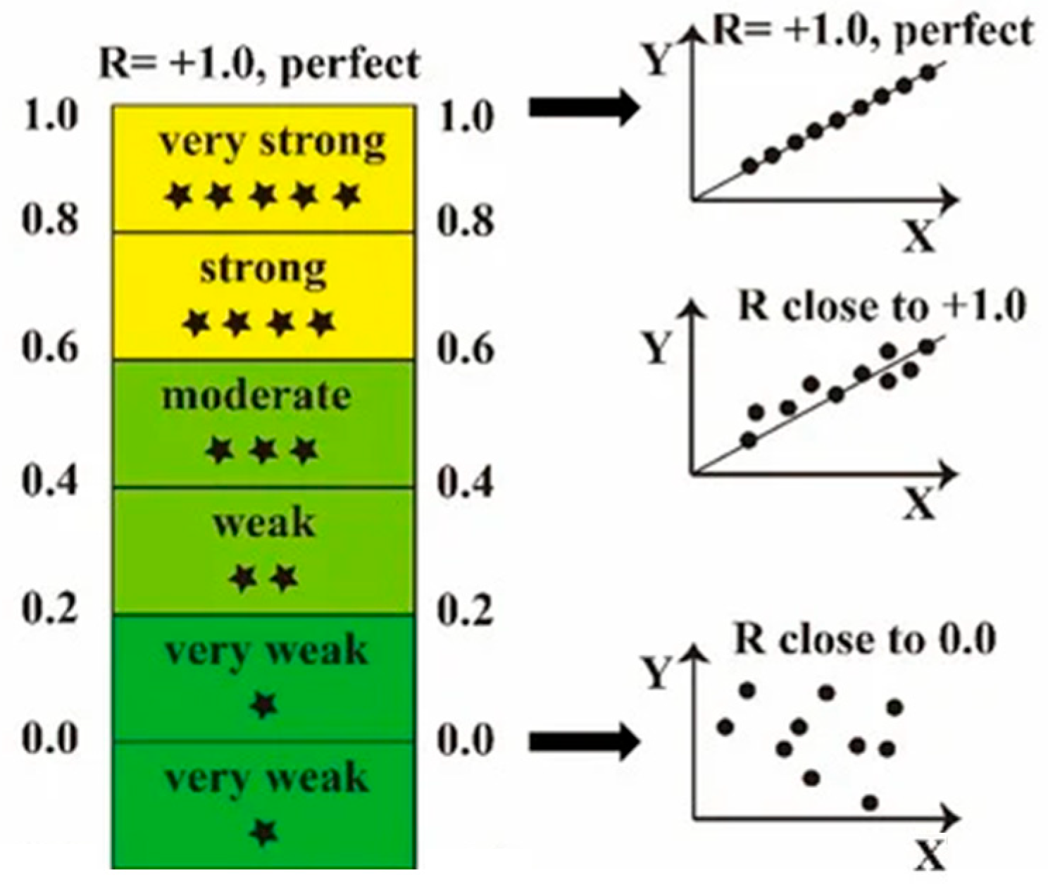
The following figure (Figure 2) shows the interpretation of the given metric.
Metrics derived from metrics or squared errors are called scale-dependent metrics. They correspond to the scale of the original data and present errors in the same unit [3]. Nevertheless, the R2 value alone is not an adequate measure to assess the validity of the model and the relationship with unexplained variance must be taken into account [24,27].
Scale-dependent metrics:
  • The Sum of Squared Errors (SSE) is a statistical measure employed to assess the quality of a model or the difference between predicted outcomes and actual data. It is often used in regression, modelling, and machine learning to quantify model error.
S S E = i = 1 n y i y ^ i 2 ,
where n represents the number of values, yi measured values and y ^ i forecasted values.
SSE does not have units comparable to the original data, so it is less intuitive for direct interpretation. To achieve this, a derivative like Mean Squared Error (MSE) or Root Mean Squared Error (RMSE) is frequently utilised.
  • Root Mean Squared Error (RMSE),
R M S E = 1 n i = 1 n y i y ^ i 2 ,
where n represents the number of values, yi measured values and y ^ i   forecasted values.
In contrast to MSE, RMSE shares the same units as the original data, which enhances its interpretability compared to MSE [28]. R2 is considered more independent than RMSE since it is not reliant on the unit, allowing for comparison among models trained on various datasets.
  • Mean Squared Error (MSE)—The value of Mean Squared Error (MSE) indicates the proximity of the regression line to a group of points. It calculates the Mean Squared Error between the predicted and actual values, assigning greater importance to larger discrepancies. When the average of the collection of errors is determined, it is referred to as the Mean Squared Error. The smaller the MSE value, the more accurate the prediction becomes. MSE is measured in units that are the square of the target variable. The units of MSE are the square of the target variable.
M S E = 1 n i = 1 n y i y ^ i 2 ,
  • Mean Absolute Error (MAE)—The Mean Absolute Error reflects the average discrepancy between the measured and forecasted values. The nearer the MAE value is to 0, the more accurate the prediction becomes [7].
M A E = 1 n i = 1 n y i y ^ i ,
  • MAPE indicates the level of accuracy of the forecasted value compared to the actual measured values [7] (expressed in percent). For the MAPE index, an effective model has a value of less than 14%.
M A P E = 1 n i = 0 n y i y ^ i y i ,
where n represents the number of values, yi measured values and   y ^ i forecasted values.
RMSE, MAE and MAPE are widely used accuracy metrics because they are easy to interpret. They offer a plausible assessment of the typical error anticipated from the predictions at each prediction stage [7].
  • SMAPE (symmetric mean absolute percentage error).
S M A P E = 1 n i = 1 n y ^ i y i y i + y ^ i 2 ,
It conveys the typical variation between the actual values yi and the estimated values   y ^ i , normalising the error relative to the average value. A limitation of SMAPE is that if the actual value or predicted value is 0, the error value will increase up to the upper error bound.
However, different accuracy metrics rely on different types of measurement. For example, MSE, RMSE and MAE calculations are based on root mean square and absolute errors. MAPE calculations are based on percentage errors. Different accuracy metrics indicate different types of quality. Because different accuracy metrics have their own strengths and weaknesses, some accuracy metrics may not be appropriate for a particular prediction model. Therefore, selecting an appropriate accuracy metric for evaluating prediction models is a critical issue [24].
When using application software, increasing the number of regression curve degrees is a trivial matter. For the monitored metrics, the values appear to be better because they achieve better values compared to previous designs. However, this increases the complexity of the model. The Akaike Information Criterion and the Bayesian Information Criterion (BIC) are used to assess the complexity of the model.

2.2.1. Akaike Information Criterion (AIC)

Model selection criteria serve as a valuable resource for identifying a model with appropriate structure and complexity from a range of potential candidates. The criterion can assess whether the selected model provides an optimal balance between goodness of fit and complexity [29]. This is the role of the information criterion. It is a general information-theoretic measure of model quality based on selection [30,31,32]. It is used when we have several models that we can use to predict the data [33,34]. Essentially, the selection criterion will discard potential models that are either too simple for the data or too complicated [29].
A I C = n l n S S E n + 2 k + 2 k ( k + 1 ) n k 1 + n l n 2 π + n
where n is number of values, k is the total number of parameters estimated in the model, and SSE is the Sum of Squared Errors.
In model design, it is possible to increase the fit of the model by adding parameters, which may result in an increase in model complexity. In this sense, AIC, AICc (corrected AIC used for small sample sizes) [30] and BIC are the most commonly used selection criteria. The goal is to achieve the simplest model with the fewest variables. This minimises the risk of excessive model complexity and prevents overfitting [28].

2.2.2. Bayesian Information Criterion (BIC)

The Bayesian Information Criterion (BIC) is a powerful model selection tool that emphasises simpler models when working with large datasets. When combined with other metrics, it provides useful insights for statistical analysis and modelling. When the true model is among the possible models, the BIC selects the true model with a probability close to 1, ensuring the selection of the correct model as the sample size increases [32].
B I C = k l n ( n ) 2 l n   ( L ) ,
where n is number of values, k is the total number of parameters estimated in the model and L is the maximum value of the model’s likelihood function.

3. Illustrative Study

The procedure for applying each of the properties described is illustrated in the following example. As part of the study of the properties of composite materials, data were obtained on the absorption of composite materials with a certain percentage of textile fibre content (10%, 20%, 30% and 40%). Usually, several models are combined and we look for the model that best fits the given phenomena [32,35]. The dataset consists of 1455 records, where the x-coordinate is the wave number and the y-coordinate is the measured absorption data obtained. More detailed information about the results and the measurement method is given in [36].
Our research framework consists of the following steps:
  • Data collection and preparation—Source data were cleaned and outliers removed prior to analysis. We assume that the data distribution is normal.
  • Visualisation—Since we have samples with different textile fibre content, we used the graphical tools of the Matlab environment and visualised the obtained data (Figure 3).
  • Model design—Using the Curve Fitter Toolbox, we will progressively analyse the suitability of each built-in function and select a suitable model based on the R2 value.
  • Validation—Quality versus balance. At this point, we will not only analyse the quality of the model but also look for a balance between the quality and complexity of the model.
The resulting graphical progression is shown in the following figure.
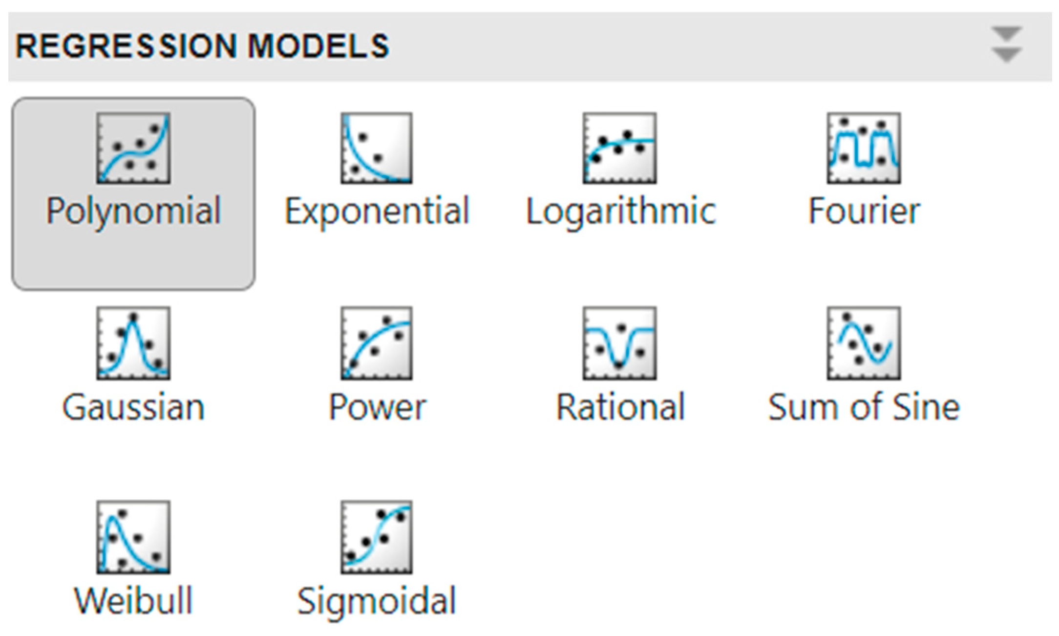
In terms of the application of mathematical modelling, conventional techniques are used to find distribution functions for data collected from experiments, including Gaussian, exponential, Laplacian, Fourier, Weibull, Wigner and Pareto [37,38]. This method is advantageous because the necessary mathematical tools are already available and integrated into various software applications. Using the specified tool, we can select the appropriate model [32]. In the Curve Fitter environment, we have several options thanks to the available toolbox libraries (Figure 4).
This environment provides metrics such as R2 (coefficient of determination), RMSE (Root Mean Square Error), visual verification using residual plots and variance distributions, and automatic parameter optimisation using various algorithms (e.g., least squares) (Figure 5). Each selection also includes options for increasing the degree.
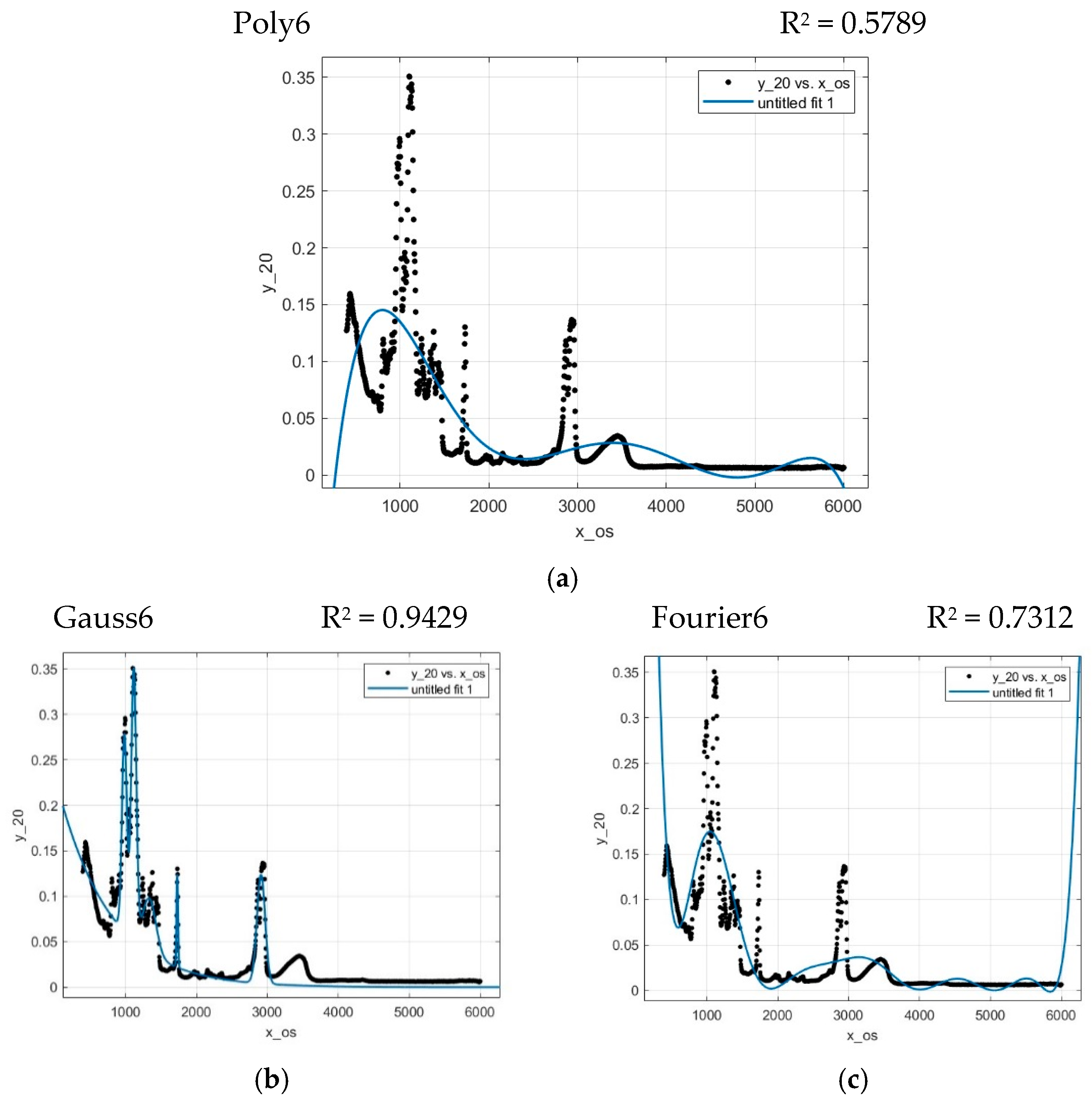
Since the search for the best model is very intuitive, we usually focus on assessing individual variants based on only one coefficient, namely R2. For a given case, possible variants were gradually considered (Figure 6).
Based on the R-squared value, we chose the Gaussian regression function as the starting method. This is a statistical approach that attempts to approximate the input-output mapping from empirical data [26]. The chosen model is interpreted by the following formula:
y = i = 1 n a i e x b i c i 2 ,
where a is the amplitude, b is the centroid (location), c is related to the peak width and n is the number of peaks.

4. Results

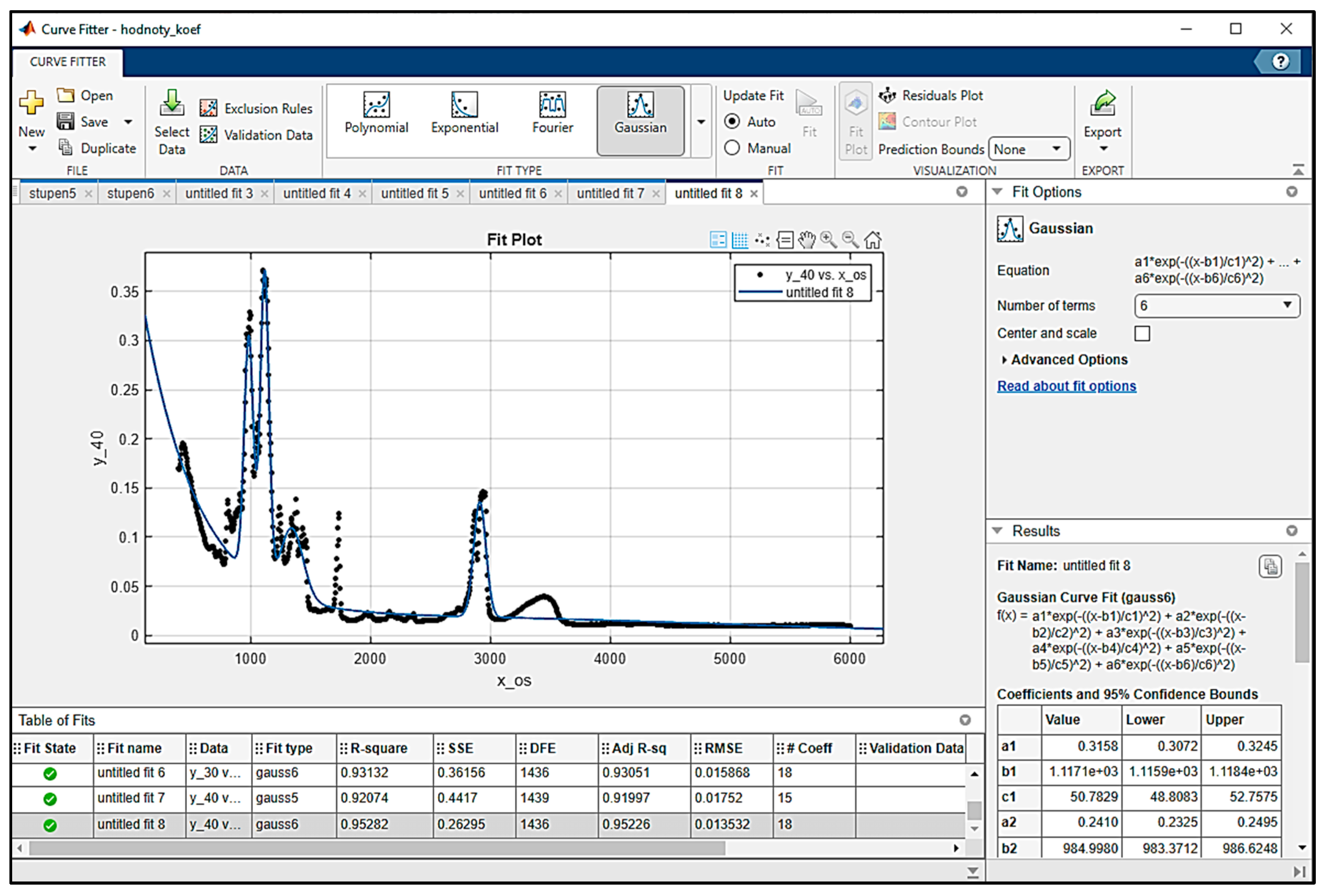
The initial selection will be made based on the value of the coefficient of determination R2. As the following figure (Figure 7) shows, we have at our disposal the individual indicators of the model and the values of the coefficients.
By gradually increasing the ‘Number of terms’, we compare the selected coefficient values. The resulting values are shown in Table 1.
Based on the table, it is clear that the more we increase the “degree”, the higher the value of the considered coefficient R2, and the values of several indicators (SSE, RMSE, MSE, SMAPE) are lower. It is therefore possible to state that the model better represents the measured data. However, it is important to assess whether this additional complexity is justified. Will we achieve a significant improvement by increasing the complexity of the model?
In this case, we can use the AIC (Akaike Information Criterion). The resulting values are shown in Table 2.
While the R2 value for the ‘gauss7’ model is higher than for ‘gauss6’, the AIC suggests that adding parameters beyond six does not significantly improve model quality.
The following values also speak in favour of the gauss6 variant:
  • MAE—a lower value of this indicator means that the model is more accurate, because its predictions are closer to the actual values.
  • MAPE expresses the error in the form of a percentage difference between the actual and predicted values, which allows easier comparison of different datasets or units. A lower value means a more accurate model.

5. Conclusions

Evaluating model suitability is a very challenging task, as there is no objective way of knowing what is a suitable model and what is not. This article has provided insight into the dynamics between simulation and validation and how these techniques can improve the overall quality and credibility of predictive models in various applications.
Specifically, this study provides an in-depth examination of the processes and tools involved in the transition from simulation to validation in predictive modelling. Using MATLAB’s Curve Fitting Toolbox as the primary environment, we demonstrated how advanced modelling and validation techniques can be applied to ensure the accuracy and reliability of predictive models. Our analysis focused on composite absorption data and highlighted the dynamics of balancing model complexity and performance.
Among the various models tested (e.g., polynomial, Gaussian, Fourier), the Gaussian regression model emerged as the most suitable, achieving a high coefficient of determination (R2 = 0.9429) for a six-parameter configuration. This reflects its superior ability to capture the underlying patterns of the data compared to other models.
Incremental increases in model complexity, represented by the number of parameters, led to improvements in key metrics such as Sum of Squared Errors (SSE), Root Mean Square Error (RMSE), Mean Squared Error (MSE) and symmetric mean absolute percentage error (SMAPE). For example, the RMSE decreased from 0.021555 (four-parameter model) to 0.013537 (six-parameter model) and the SSE decreased from 0.675565 to 0.266441 over the same range. The SMAPE showed improvements, decreasing from 0.000442 to 0.000343, indicating greater agreement between predicted and actual values.
We can also see that while increasing the number of parameters to 7 further reduced errors and improved R2 to 0.94663, the Akaike Information Criterion (AIC) showed diminishing returns in model performance relative to complexity. The AIC for the six-parameter model (−2806.93) was significantly better than that for the seven-parameter model (−2847.17), highlighting the importance of parsimony in model selection.
In addition, metrics such as MAPE and MAE also supported the selection of the six-parameter model as optimal for balancing accuracy with practical applicability.
These results demonstrate the importance of systematically evaluating model performance across multiple dimensions. While a higher R2 can be appealing, relying solely on this metric can lead to overly complex models that may lack interpretability and robustness. Instead, integrating a range of metrics, including SSE, RMSE, AIC and BIC, ensures a balanced approach to model validation.
Future work could explore larger datasets, different application domains, or alternative modelling frameworks to generalise these findings. In addition, the incorporation of real-time data streams or ensemble modelling techniques could further improve the accuracy and reliability of predictions. We will also focus on evaluating the residuals and statistical significance of individual parameters affecting the balance between model quality and complexity. This study provides a basis for improving model evaluation procedures and highlights the need for robust validation protocols to ensure that predictive models provide practical and reliable solutions in various scientific and engineering fields.

Author Contributions

Conceptualisation, S.H. and K.A.; methodology, S.H. and K.A.; software, J.H. and A.V.; validation, S.H., K.A. and J.H.; formal analysis, A.V.; investigation, S.H. and K.A.; resources, S.H. and J.H.; data curation, K.A.; writing—original draft preparation, S.H.; writing—review and editing, S.H. and K.A.; visualisation, S.H. and A.V.; supervision, K.A.; project administration, K.A. and J.H.; funding acquisition, J.H. All authors have read and agreed to the published version of the manuscript.

Funding

This work was supported by the Slovak Research and Development Agency under contract No. APVV-23-0591, and by the projects VEGA 1/0704/22 and KEGA 014TUKE-4/2023 granted by the Ministry of Education, Science, Research, and Sport of the Slovak Republic.

Institutional Review Board Statement

Not applicable.

Informed Consent Statement

Not applicable.

Data Availability Statement

The original contributions presented in this study are included in the article. Further inquiries can be directed to the corresponding author.

Conflicts of Interest

The authors declare no conflicts of interest.

References

  1. Al-Marshadi, A.H.; Alharby, A.H.; Shahbaz, M.Q. Selecting the “true” regression model: A new ranking method. Adv. Appl. Stat. 2023, 87, 1–11. [Google Scholar] [CrossRef]
  2. Vagaská, A.; Gombár, M.; Straka, Ľ. Selected Mathematical Optimization Methods for Solving Problems of Engineering Practice. Energies 2022, 15, 2205. [Google Scholar] [CrossRef]
  3. Sargent, R.G. Verification, Validation, and Accreditation of Simulation Models. In Proceedings of the 2000 Winter Simulation Conference, Orlando, FL, USA, 10–13 December 2000; Volume 1, pp. 50–59. [Google Scholar] [CrossRef]
  4. Hošovský, A.; Pite, J.; Adámek, M.; Mižáková, J.; Židek, K. Comparative study of week-ahead forecasting of daily gas consumption in buildings using regression ARMA/SARMA and genetic-algorithm-optimized regression wavelet neural network models. J. Build. Eng. 2021, 34, 101955. [Google Scholar] [CrossRef]
  5. Pavlenko, I.; Piteľ, J.; Ivanov, V.; Berladir, K.; Mižáková, J.; Kolos, V.; Trojanowska, J. Using Regression Analysis for Automated Material Selection in Smart Manufacturing. Mathematics 2022, 10, 1888. [Google Scholar] [CrossRef]
  6. Hrehova, S.; Vagaska, A. Computer Models as Appropriate Tools in Elearning. In Proceedings of the INTED2017 Proceedings, Valencia, Spain, 6–8 March 2017; pp. 8871–8877. [Google Scholar]
  7. Piotrowski, P.; Rutyna, I.; Baczyński, D.; Kopyt, M. Evaluation Metrics for Wind Power Forecasts: A Comprehensive Review and Statistical Analysis of Errors. Energies 2022, 15, 9657. [Google Scholar] [CrossRef]
  8. Tako, A.; Tsioptsias, N.; Robinson, S. Can we learn from simple simulation models? An experimental study on user learning. J. Simul. 2020, 14, 130–144. [Google Scholar] [CrossRef]
  9. Robinson, S. Exploring the relationship between simulation model accuracy and complexity. J. Oper. Res. Soc. 2022, 74, 1992–2011. [Google Scholar] [CrossRef]
  10. Priesmann, J.; Nolting, L.; Praktiknjo, A. Are complex energy system models more accurate? An intra-model comparison of power system optimization models. Appl. Energy 2019, 255, 113783. [Google Scholar] [CrossRef]
  11. Zhang, L. Analysis of the trade-off between accuracy and complexity of identified models of dynamic systems. Anal. Data Process. Syst. 2024, 94, 85–93. [Google Scholar] [CrossRef]
  12. Rohskopf, A.; Goff, J.; Sema, D.; Gordiz, K.; Nguyen, N.; Henry, A.; Thompson, A.; Wood, M. Exploring model complexity in machine learned potentials for simulated properties. J. Mater. Res. 2023, 38, 5136–5150. [Google Scholar] [CrossRef]
  13. Trojanová, M.; Hošovský, A.; Čakurda, T. Evaluation of Machine Learning-Based Parsimonious Models for Static Modeling of Fluidic Muscles in Compliant Mechanisms. Mathematics 2023, 11, 149. [Google Scholar] [CrossRef]
  14. Hrehova, S.; Husár, J.; Knapčíková, L. The Fuzzy Logic Predictive Model for Remote Increasing Energy Efficiency. Mob. Netw. Appl. 2023, 28, 1293–1305. [Google Scholar] [CrossRef]
  15. Rodríguez-Martín, M.; Fueyo, J.G.; Gonzalez-Aguilera, D.; Madruga, F.J.; García-Martín, R.; Muñóz, Á.L.; Pisonero, J. Predictive Models for the Characterization of Internal Defects in Additive Materials from Active Thermography Sequences Supported by Machine Learning Methods. Sensors 2020, 20, 3982. [Google Scholar] [CrossRef] [PubMed]
  16. Knapcikova, L.; Behunova, A.; Behun, M. Using a discrete event simulation as an effective method applied in the production of recycled material. Adv. Prod. Eng. Manag. 2020, 15, 431–440. [Google Scholar] [CrossRef]
  17. Greene, W.H. Econometric Analysis, 7th ed.; Pearson Education Limited: Edinburgh, UK, 2012; pp. 383–494. [Google Scholar]
  18. Hsiao, C.-W.; Chan, Y.-C.; Lee, M.-Y.; Lu, H.-P. Heteroscedasticity and Precise Estimation Model Approach for Complex Financial Time-Series Data: An Example of Taiwan Stock Index Futures before and during COVID-19. Mathematics 2021, 9, 2719. [Google Scholar] [CrossRef]
  19. Belkin, M.; Hsu, D.; Mitra, P.P. Overfitting or Perfect Fitting? Risk Bounds for Classification and Regression Rules that Interpolate. arXiv 2018, arXiv:1806.05161. [Google Scholar] [CrossRef]
  20. Donald, S.; Lang, K. Inference with Difference-in-Differences and Other Panel Data. Rev. Econ. Stat. 2007, 89, 221–233. [Google Scholar] [CrossRef]
  21. Im, K.S.; Pesaran, M.; Shin, Y. Testing for unit roots in heterogeneous panels. J. Econ. 2003, 115, 53–74. [Google Scholar] [CrossRef]
  22. Adamczak, M.; Kolinski, A.; Trojanowska, J.; Husár, J. Digitalization Trend and Its Influence on the Development of the Operational Process in Production Companies. Appl. Sci. 2023, 13, 1393. [Google Scholar] [CrossRef]
  23. Lazár, I.; Husár, J. Validation of the serviceability of the manufacturing system using simulation. J. Effic. Responsib. Educ. Sci. 2012, 5, 252–261. [Google Scholar] [CrossRef]
  24. Jierula, A.; Wang, S.; OH, T.-M.; Wang, P. Study on Accuracy Metrics for Evaluating the Predictions of Damage Locations in Deep Piles Using Artificial Neural Networks with Acoustic Emission Data. Appl. Sci. 2021, 11, 2314. [Google Scholar] [CrossRef]
  25. Carrera, B.; Kim, K. Comparison Analysis of Machine Learning Techniques for Photovoltaic Prediction Using Weather Sensor Data. Sensors 2020, 20, 3129. [Google Scholar] [CrossRef]
  26. Asante-Okyere, S.; Shen, C.; Yevenyo Ziggah, Y.; Moses Rulegeya, M.; Zhu, X. Investigating the Predictive Performance of Gaussian Process Regression in Evaluating Reservoir Porosity and Permeability. Energies 2018, 11, 3261. [Google Scholar] [CrossRef]
  27. Trojanowski, P. Comparative analysis of the impact of road infrastructure development on road safety—A case study. Sci. J. Marit. Univ. Szczecin 2020, 63, 23–28. [Google Scholar] [CrossRef]
  28. Rajamanickam, V.; Babel, H.; Montano-Herrera, L.; Ehsani, A.; Stiefel, F.; Haider, S.; Presser, B.; Knapp, B. About Model Validation in Bioprocessing. Processes 2021, 9, 961. [Google Scholar] [CrossRef]
  29. St-Aubin, P.; Agard, B. Precision and Reliability of Forecasts Performance Metrics. Forecasting 2022, 4, 882–903. [Google Scholar] [CrossRef]
  30. Cavanaugh, J.E.; Neath, A.A. The Akaike information criterion: Background, derivation, properties, application, interpretation, and refinements. WIREs Comput Stat. 2019, 11, e1460. [Google Scholar] [CrossRef]
  31. Folz, B. Multiple Regression. Available online: https://www.youtube.com/watch?v=-BR4WElPIXg (accessed on 25 November 2024).
  32. Marliana, R.R.; Suhayati, M.; Ningsih, S.B.H. Schwarz’s Bayesian Information Criteria: A Model Selection Between Bayesian-SEM and Partial Least Squares-SEM. Pak. J. Stat. Oper. Res. 2023, 19, 637–648. [Google Scholar] [CrossRef]
  33. Kronova, J.; Izarikova, G.; Trebuna, P.; Pekarcikova, M.; Filo, M. Application Cluster Analysis as a Support form Modelling and Digitalizing the Logistics Processes in Warehousing. Appl. Sci. 2024, 14, 4343. [Google Scholar] [CrossRef]
  34. Ondov, M.; Rosova, A.; Sofranko, M.; Feher, J.; Cambal, J.; Feckova Skrabulakova, E. Redesigning the Production Process Using Simulation for Sustainable Development of the Enterprise. Sustainability 2022, 14, 1514. [Google Scholar] [CrossRef]
  35. Mesarosova, J.; Martinovicova, K.; Fidlerova, H.; Chovanova, H.H.; Babcanova, D.; Samakova, J. Improving the level of predictive maintenance maturity matrix in industrial enterprise. Acta Logist. 2022, 9, 183–193. [Google Scholar] [CrossRef]
  36. Hrehova, S.; Knapčíková, L. Design of Mathematical Model and Selected Coefficient Specifications for Composite Materials Reinforced with Fabric from Waste Tyres. Materials 2023, 16, 5046. [Google Scholar] [CrossRef] [PubMed]
  37. Isametova, M.E.; Nussipali, R.; Martyushev, N.V.; Malozyomov, B.V.; Efremenkov, E.A.; Isametov, A. Mathematical Modeling of the Reliability of Polymer Composite Materials. Mathematics 2022, 10, 3978. [Google Scholar] [CrossRef]
  38. Filina-Dawidowicz, L.; Sęk, J.; Trojanowski, P.; Wiktorowska-Jasik, A. Conditions of Decision-Making Related to Implementation of Hydrogen-Powered Vehicles in Urban Transport: Case Study of Poland. Energies 2024, 17, 3450. [Google Scholar] [CrossRef]
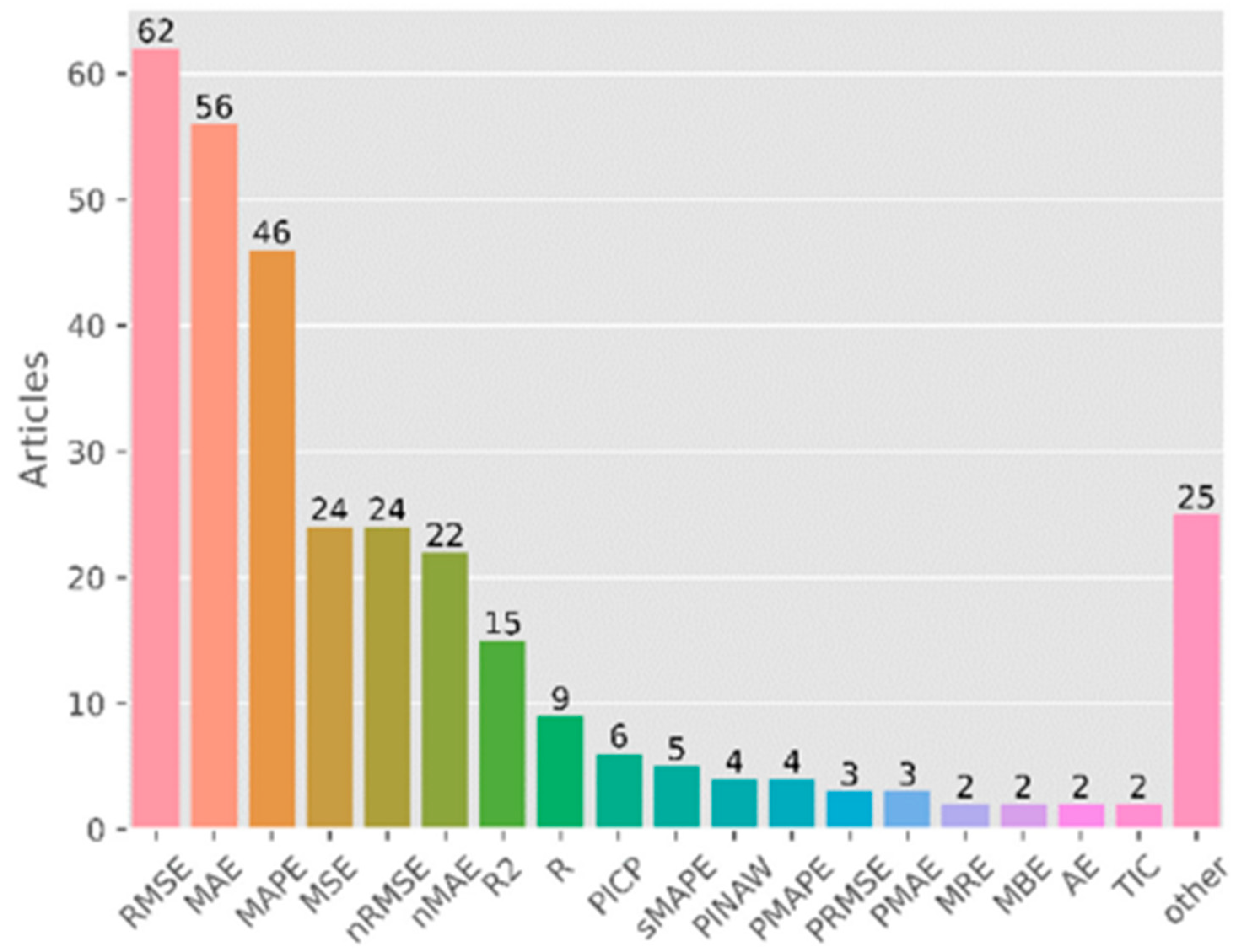
Figure 1. Overview of metrics usage based on a previous study [7].
Applsci 15 03107 g001
Figure 2. Interpretation of R squared [26].
Applsci 15 03107 g002
Figure 3. Measured absorption values with detail of the upper part [36].
Applsci 15 03107 g003
Figure 4. Model design tools in the Curve Fitter environment.
Applsci 15 03107 g004
Figure 5. Selected values of some metrics.
Applsci 15 03107 g005
Figure 6. Graphical display of selected models, (a) Polynomial model, (b) Gaussian model, (c) Fourier series model.
Applsci 15 03107 g006
Figure 7. Basic model in the Curve Fitting Toolbox environment.
Applsci 15 03107 g007
Table 1. Results of scenarios.
Number of Coefficients
4567
R20.8553150.9291220.9429370.94663
adjR20.8549160.9288770.9427000.946371
SSE0.6755650.3309450.2664410.249196
RMSE0.0215550.0150870.0135370.013091
MSE0.0004650.0002280.0001830.000171
MAE0.0059920.0067010.0048850.007245
MAPE0.0139360.0140610.0117190.013945
SMAPE0.0004420.0003640.0003430.000333
Table 2. Results of AIC.
Number of Coefficients
4567
R20.8553150.9291220.9429370.94663
adjR20.8549160.9288770.9427000.946371
AIC−2223.45−2672.05−2806.93−2847.17
Disclaimer/Publisher’s Note: The statements, opinions and data contained in all publications are solely those of the individual author(s) and contributor(s) and not of MDPI and/or the editor(s). MDPI and/or the editor(s) disclaim responsibility for any injury to people or property resulting from any ideas, methods, instructions or products referred to in the content.