

An Aeromagnetic Compensation Algorithm Based on a Temporal Convolutional Network


Abstract
1. Introduction
2. Materials and Methods
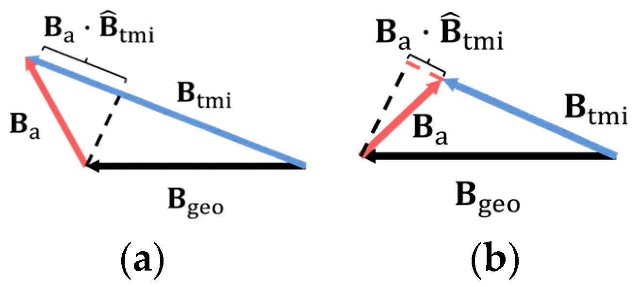
2.1. Tolles–Lawson Model
2.2. MagTCN
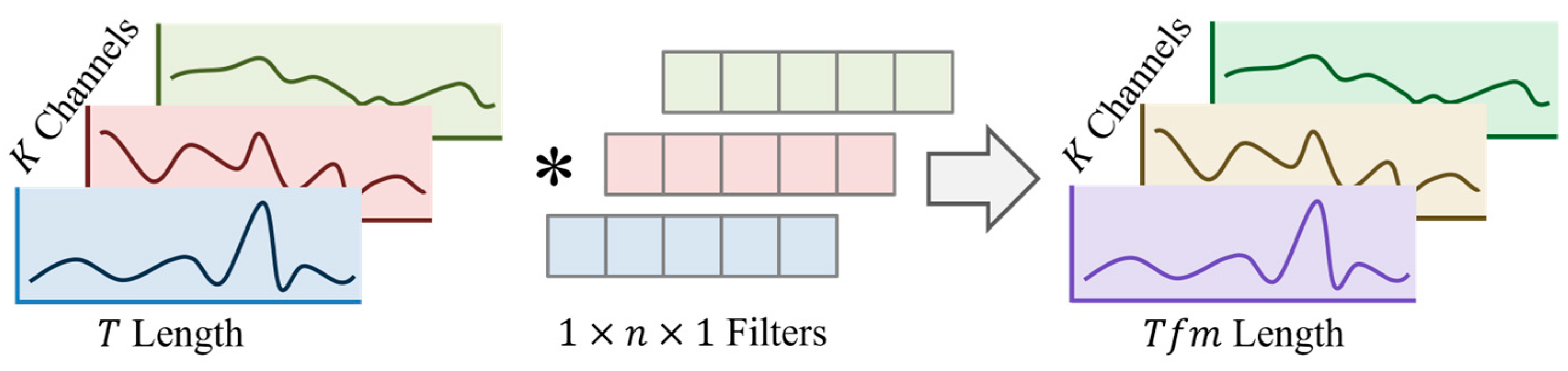
2.2.1. Separable Convolution Module
2.2.2. Gaussian Error Linear Unit
2.2.3. Reversible Instance Normalization Module
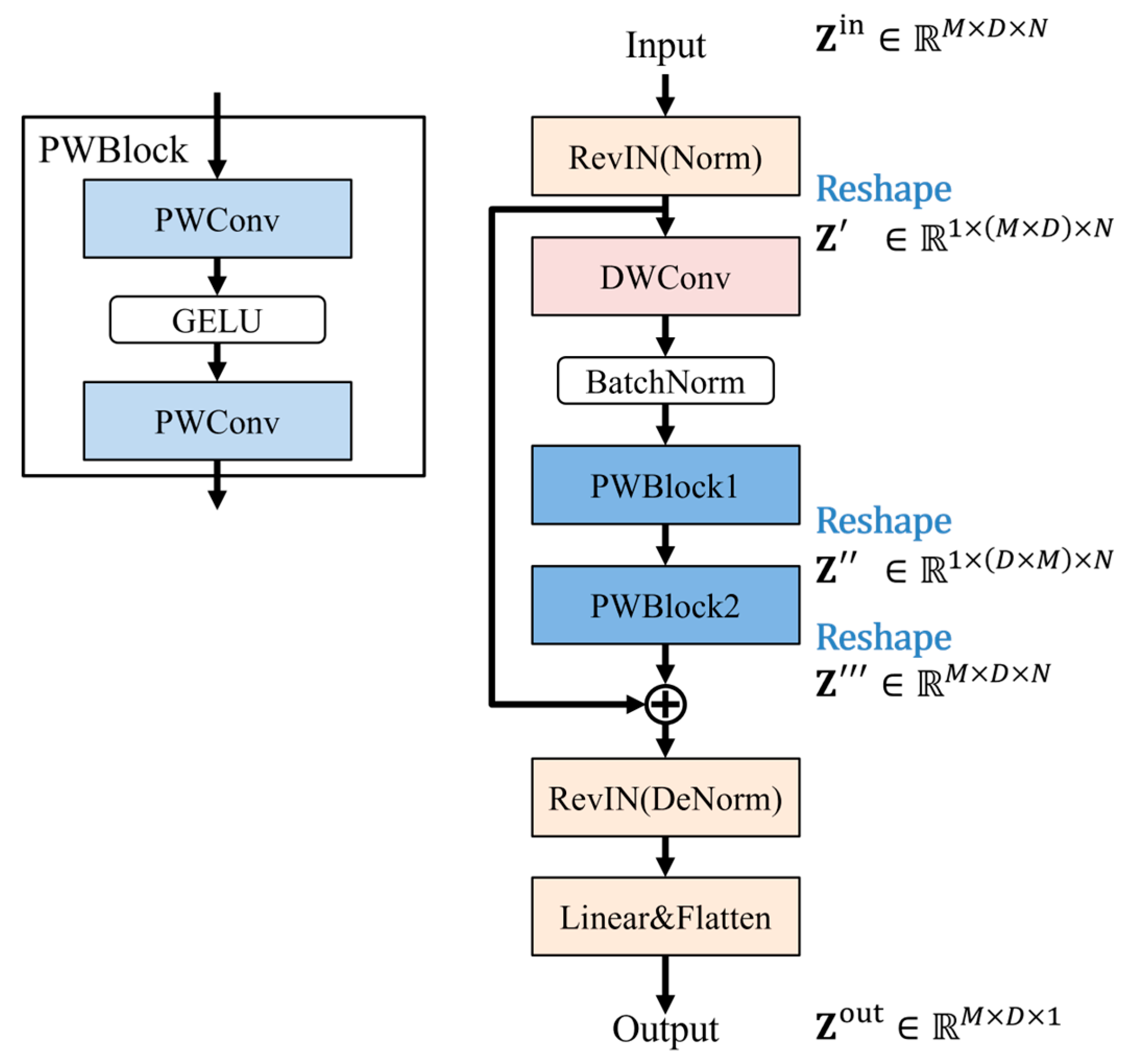
2.2.4. The Structure of MagTCN
2.3. Loss Function
3. Experimental Details
3.1. Data Preparation
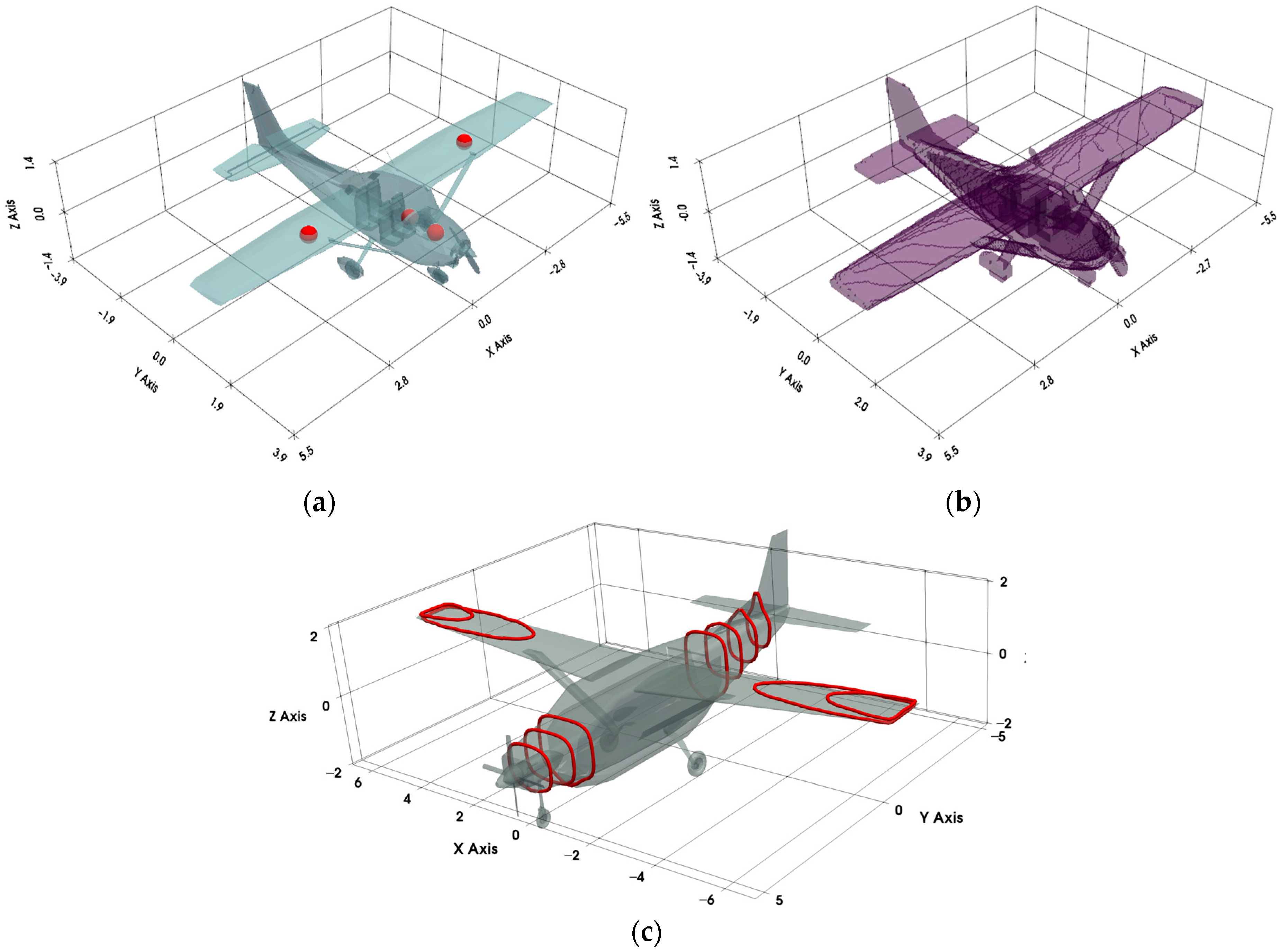
3.1.1. Simulation Dataset
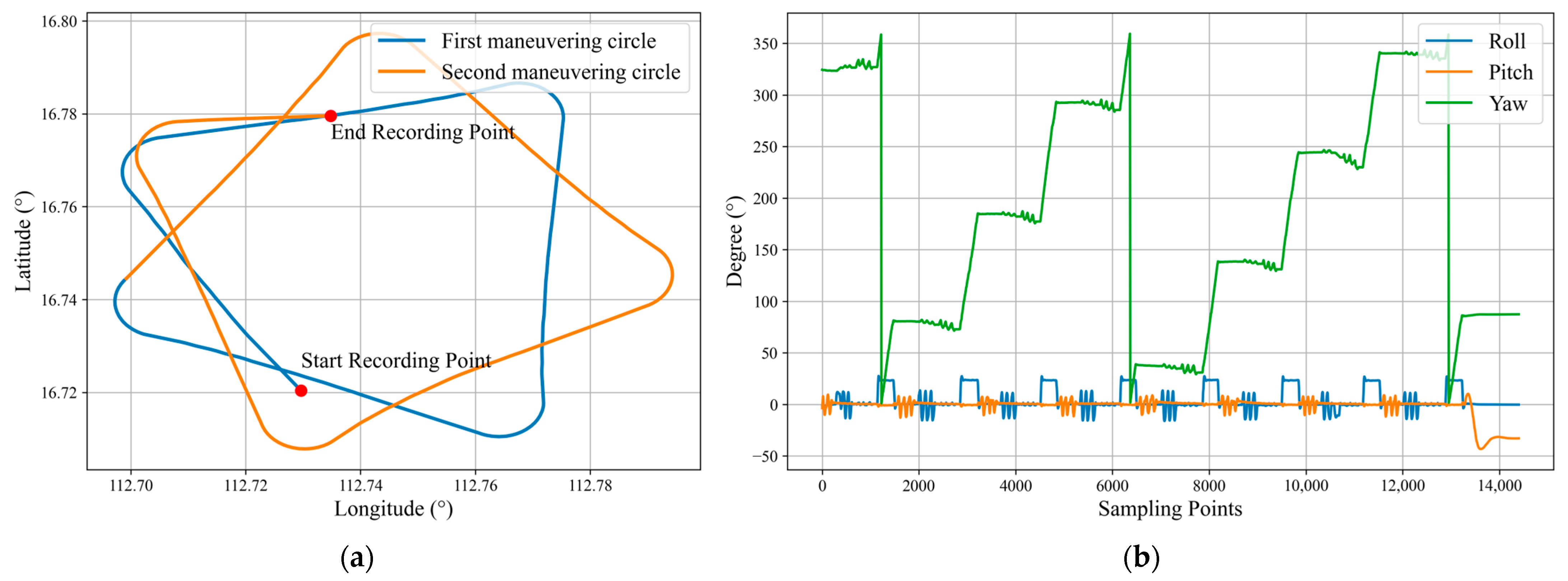
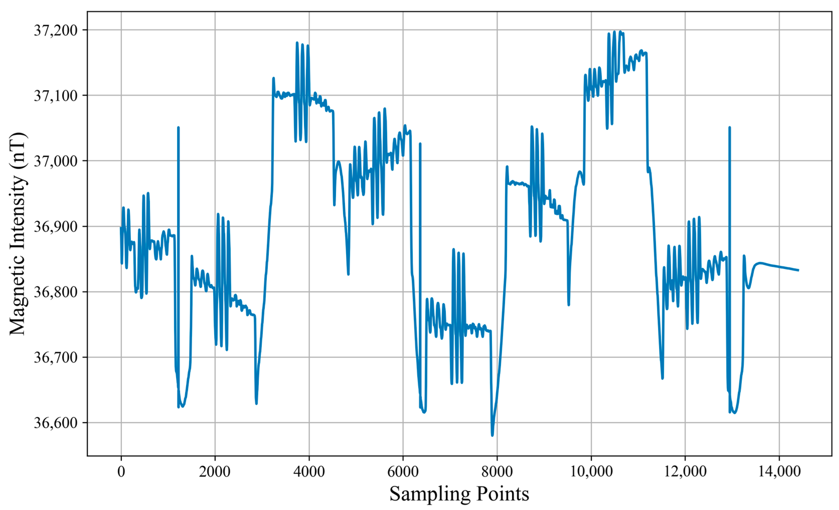
3.1.2. Real Dataset
3.2. Model Parameters
3.3. Evaluation Metrics
4. Results and Discussion
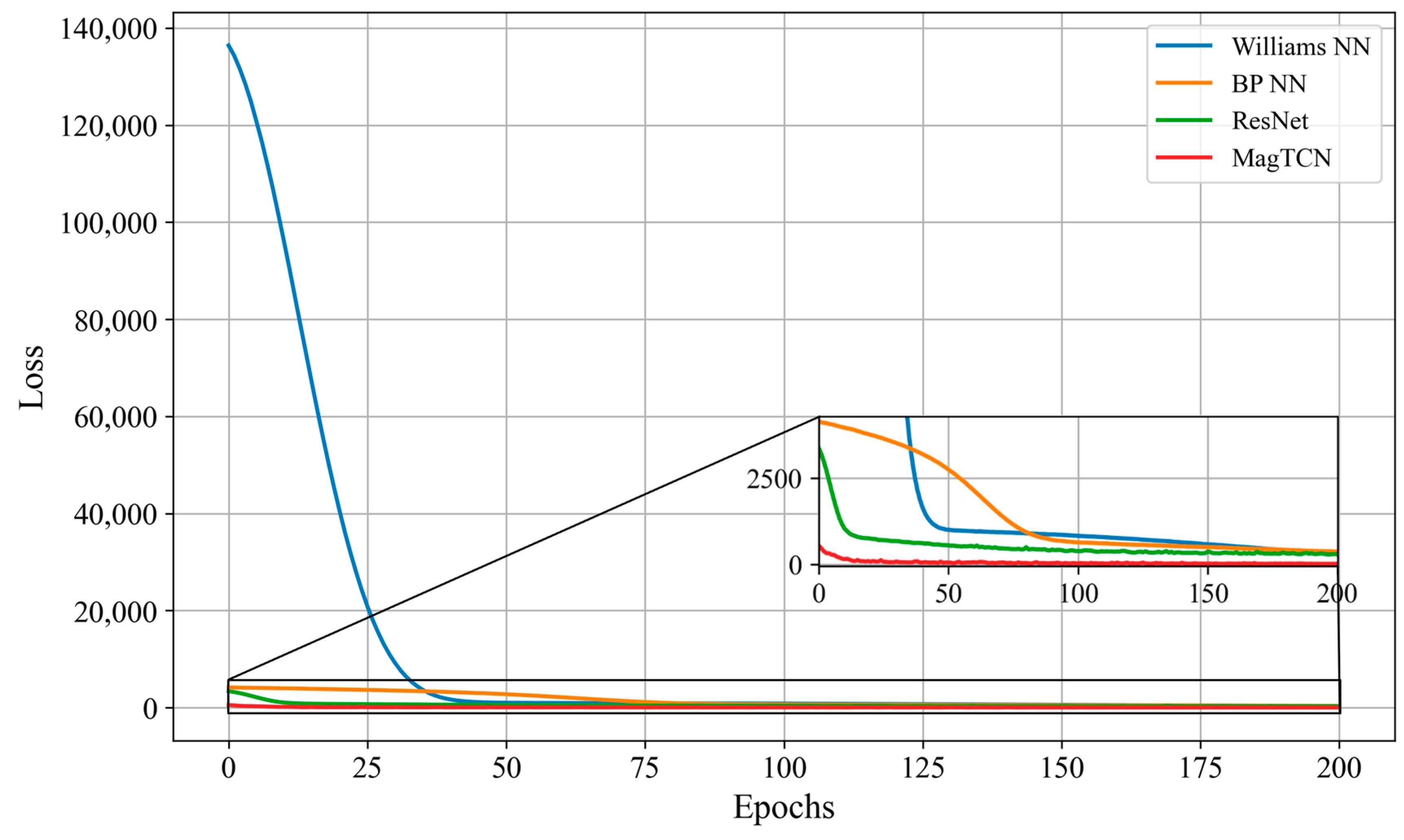
4.1. Simulation Dataset Test Results
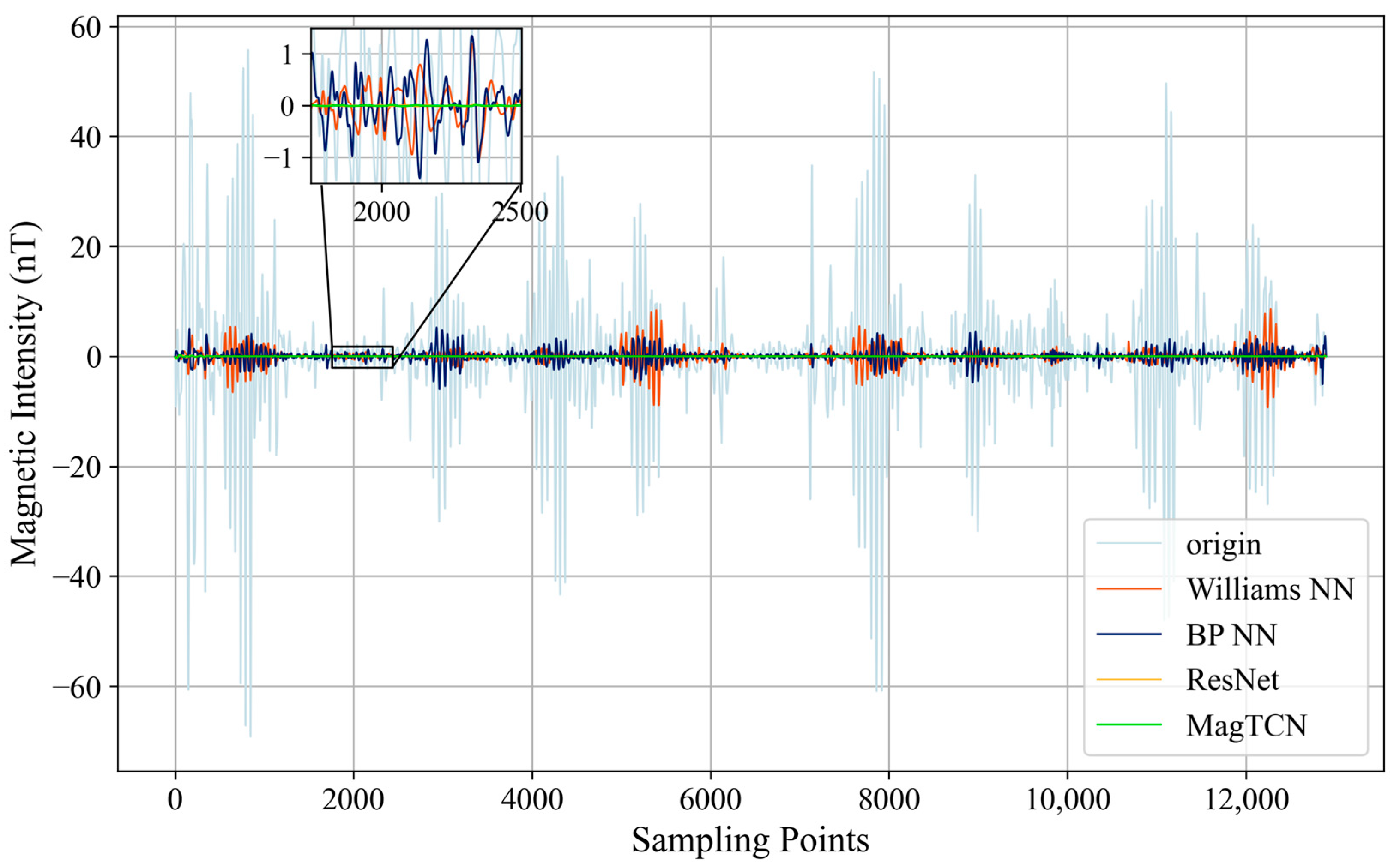
4.2. DAF-MIT AIA Open Flight Data Test Results for Flight 1002.20
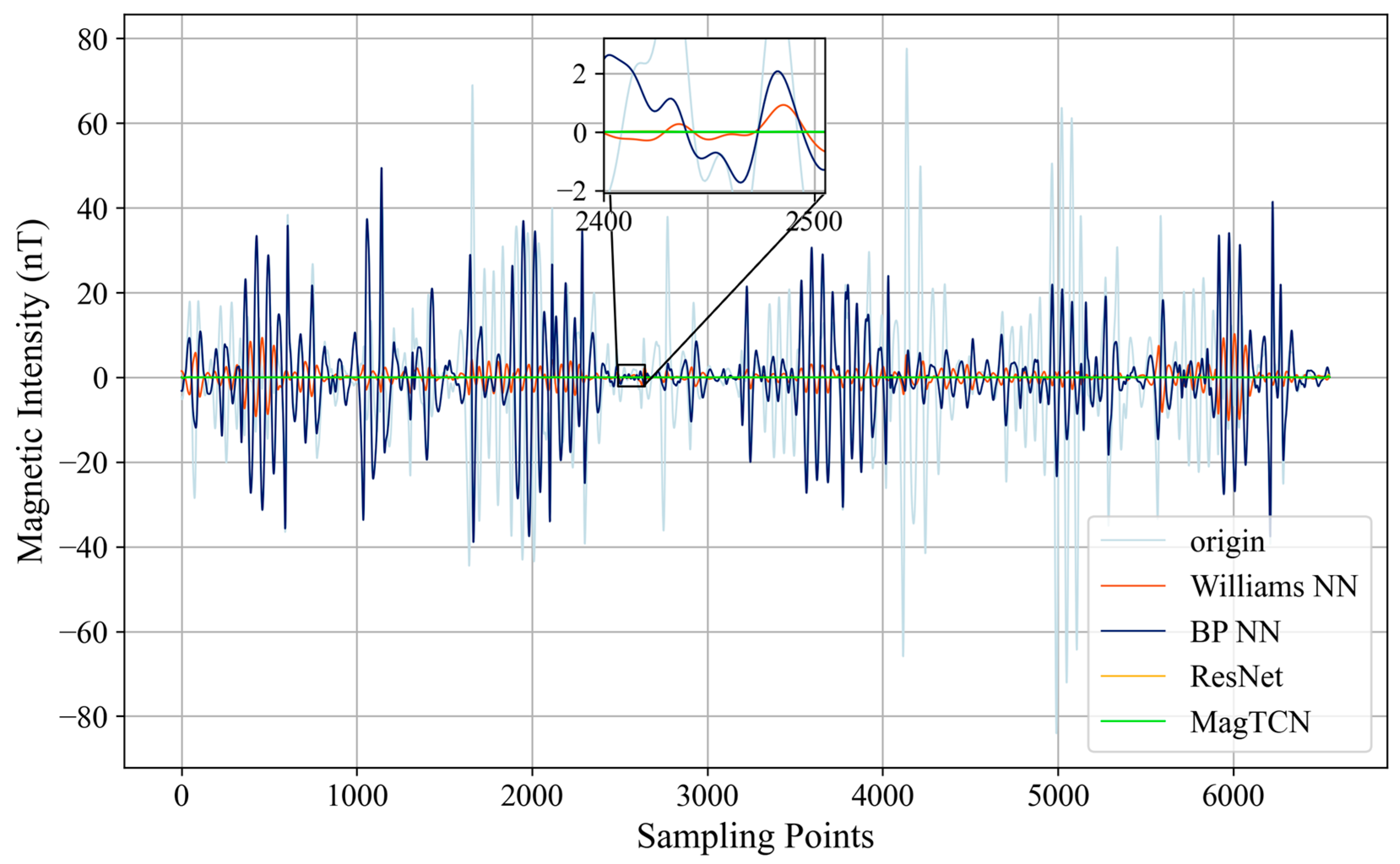
4.3. DAF-MIT AIA Open Flight Data Test Results for Flight 1006.06
4.4. Compensation Algorithm Resource Consumption Test Results
5. Conclusions
Author Contributions
Funding
Institutional Review Board Statement
Informed Consent Statement
Data Availability Statement
Acknowledgments
Conflicts of Interest
References
- Tolles, W.E.; Lawson, J.D. Magnetic Compensation of MAD Equipped Aircraft; Airborne Instruments Lab. Inc.: Mineola, NY, USA, 1950; p. 201. [Google Scholar]
- Tolles, W.E. Compensation of Aircraft Magnetic Fields. U.S. Patent 2,692,970, 26 October 1954. [Google Scholar]
- Tolles, W.E. Magnetic Field Compensation System. U.S. Patent 2,706,801, 19 April 1955. [Google Scholar]
- Tolles, W.E. Eddy-Current Compensation. U.S. Patent 2,802,983, 13 August 1957. [Google Scholar]
- Leliak, P. Identification and evaluation of magnetic-field sources of magnetic airborne detector equipped aircraft. IRE Trans. Aerosp. Navig. Electron. 1961, ANE-8, 95–105. [Google Scholar] [CrossRef]
- Leach, B.W. Aeromagnetic compensation as a linear regression problem. In Information Linkage Between Applied Mathematics and Industry; Elsevier: Amsterdam, The Netherlands, 1980; pp. 139–161. [Google Scholar]
- Feng, Y.; Zhang, Q.; Zheng, Y.; Qu, X.; Wu, F.; Fang, G. An improved aeromagnetic compensation method robust to geomagnetic gradient. Appl. Sci. 2022, 12, 1490. [Google Scholar] [CrossRef]
- Chen, B.; Zhang, K.; Yan, B.; Zhu, W. The Conjunctive Compensation Method Based on Inertial Navigation System and Fluxgate Magnetometer. Appl. Sci. 2023, 13, 5138. [Google Scholar] [CrossRef]
- Chen, B.; Huang, L.; Zhang, K.; Hu, J.; Zhu, W. Magnetic interference analysis and compensation method of airborne electronic equipment in an unmanned aerial vehicle. Appl. Sci. 2023, 13, 7455. [Google Scholar] [CrossRef]
- Williams, P.M. Aeromagnetic compensation using neural networks. Neural Comput. Appl. 1993, 1, 207–214. [Google Scholar] [CrossRef]
- Bickel, S.H. Small signal compensation of magnetic fields resulting from aircraft maneuvers. IEEE Trans. Aerosp. Electron. Syst. 2007, AES-15, 518–525. [Google Scholar] [CrossRef]
- Ma, M.; Zhou, Z.; Cheng, D. A dual estimate method for aeromagnetic compensation. Meas. Sci. Technol. 2017, 28, 115904. [Google Scholar] [CrossRef]
- Xu, X.; Huang, L.; Liu, X.; Fang, G. Deepmad: Deep learning for magnetic anomaly detection and denoising. IEEE Access 2020, 8, 121257–121266. [Google Scholar] [CrossRef]
- Yu, P.; Zhao, X.; Jia, J.; Zhou, S. An improved neural network method for aeromagnetic compensation. Meas. Sci. Technol. 2021, 32, 045106. [Google Scholar] [CrossRef]
- Li, L.; Xu, Q.; Gu, H.; Zhou, L.; Liu, Z.; Cao, L. Aeromagnetic compensation algorithm based on levenberg-marquard neural network. J. Geod. Geoinf. Sci. 2021, 4, 74–83. [Google Scholar]
- Yu, P.; Bi, F.; Jiao, J.; Zhao, X.; Zhou, S.; Su, Z. An Aeromagnetic Compensation Algorithm Based on a Residual Neural Network. Appl. Sci. 2022, 12, 10759. [Google Scholar] [CrossRef]
- Zhou, S.; Yang, C.; Su, Z.; Yu, P.; Jiao, J. An aeromagnetic compensation algorithm based on radial basis function artificial neural network. Appl. Sci. 2022, 13, 136. [Google Scholar] [CrossRef]
- Jiao, J.; Yu, P.; Zhao, X.; Bi, F. Real-time aeromagnetic compensation with compressed and accelerated neural networks. IEEE Geosci. Remote Sens. Lett. 2022, 19, 1–5. [Google Scholar] [CrossRef]
- Wang, Q.; Song, J.; Zuo, C.; Dong, K.; Jin, F. An Aeromagnetic Compensation Algorithm Based on Broad Learning System. In Proceedings of the 2024 3rd International Conference on Robotics, Artificial Intelligence and Intelligent Control (RAIIC), Mianyang, China, 5–7 July 2024; pp. 373–377. [Google Scholar]
- Gnadt, A.R.; Belarge, J.; Canciani, A.J.; Conger, L.; Curro II, J.A.; Edelman, A.; Morales, P.; O’Keeffe, M.F.; Taylor, J.; Jacobs, D. DAF-MIT AIA Open Flight Data for Magnetic Navigation Research. Available online: https://zenodo.org/records/12723700 (accessed on 7 February 2025).
- Gnadt, A. Machine learning-enhanced magnetic calibration for airborne magnetic anomaly navigation. In Proceedings of the AIAA SciTech 2022 Forum, San Diego, CA, USA, 3–7 January 2022; p. 1760. [Google Scholar]
- Wang, Y.; Han, Q.; Zhan, D.; Li, Q. A data-driven OBE magnetic interference compensation method. Sensors 2022, 22, 7732. [Google Scholar] [CrossRef] [PubMed]
- Li, Q.; Zhang, L.; Liu, S. A-TCN: Attention-Based TCN for OSS Reliability Prediction on High-Dimensional Fault Dataset. In Proceedings of the 2024 IEEE 24th International Conference on Software Quality, Reliability, and Security Companion (QRS-C), Cambridge, UK,, 1–5 July 2024; pp. 187–195. [Google Scholar]
- Xiang, X.; Li, X.; Zhang, Y.; Hu, J. A short-term forecasting method for photovoltaic power generation based on the TCN-ECANet-GRU hybrid model. Sci. Rep. 2024, 14, 6744. [Google Scholar] [CrossRef] [PubMed]
- Wei, X.; Wang, Z. TCN-attention-HAR: Human activity recognition based on attention mechanism time convolutional network. Sci. Rep. 2024, 14, 7414. [Google Scholar] [CrossRef] [PubMed]
- Larsson, J. Electromagnetics from a quasistatic perspective. Am. J. Phys. 2007, 75, 230–239. [Google Scholar] [CrossRef]
- Chollet, F. Xception: Deep learning with depthwise separable convolutions. In Proceedings of the IEEE Conference on Computer Vision and Pattern Recognition, Honolulu, HI, USA, 21–26 July 2017; pp. 1251–1258. [Google Scholar]
- Hendrycks, D.; Gimpel, K. Gaussian error linear units (gelus). arXiv 2016, arXiv:1606.08415. [Google Scholar]
- Kim, T.; Kim, J.; Tae, Y.; Park, C.; Choi, J.-H.; Choo, J. Reversible instance normalization for accurate time-series forecasting against distribution shift. In Proceedings of the International Conference on Learning Representations, Vienna, Austria, 4 May 2021. [Google Scholar]
- Vaswani, A.; Shazeer, N.; Parmar, N.; Uszkoreit, J.; Jones, L.; Gomez, A.N.; Kaiser, Ł.; Polosukhin, I. Attention is all you need. Adv. Neural Inf. Process. Syst. 2017, 30, 5998–6008. [Google Scholar]
- Vassilieva, N. Characterization and Benchmarking of Deep Learning. 2017. Available online: https://www.hpcuserforum.com/presentations/Wisconsin2017/HPDLCookbook4HPCUserForum.pdf (accessed on 7 February 2025).


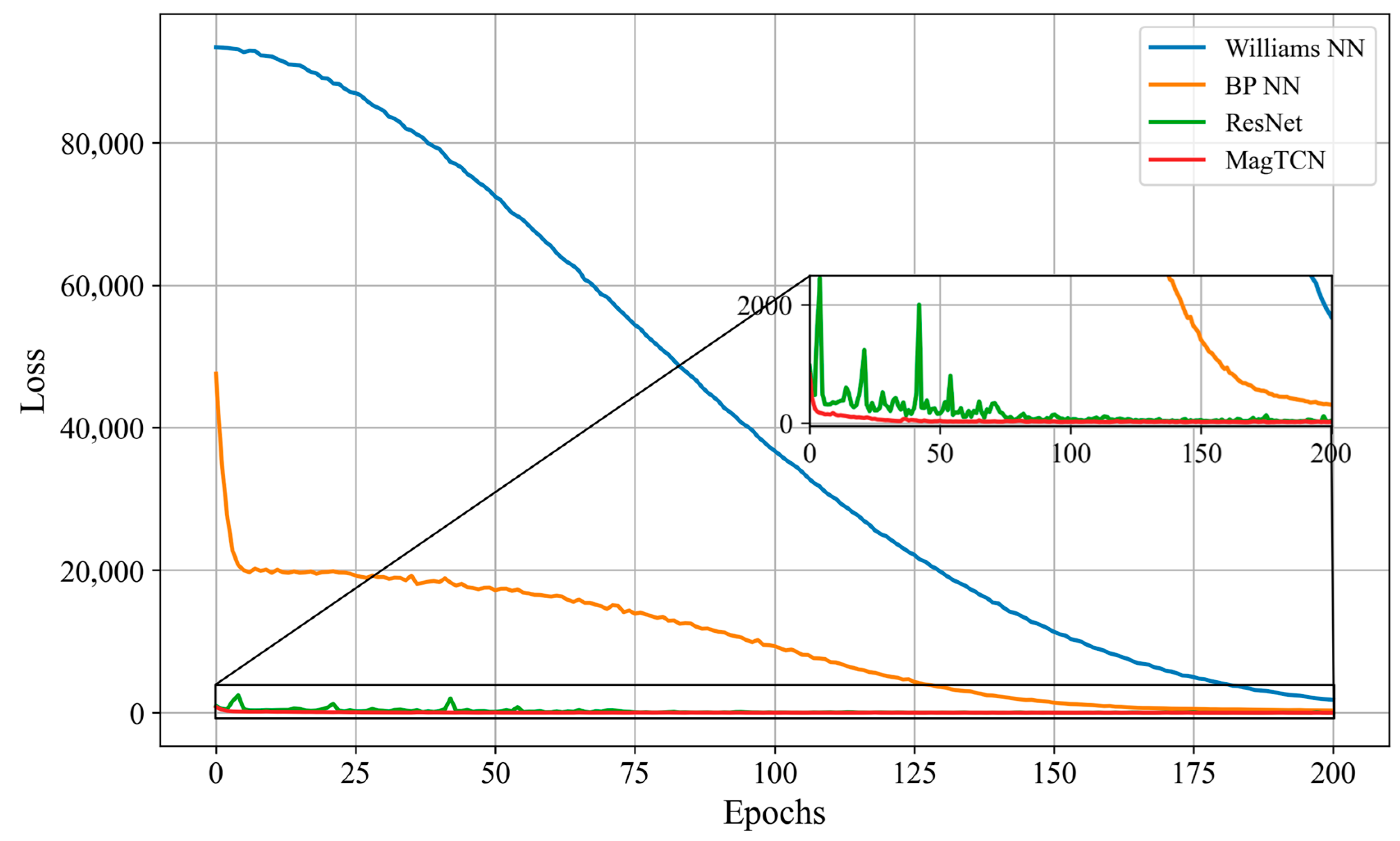
| Epoch | WilliamsNN Loss | BPNN Loss | ResNet Loss | MagTCN Loss |
|---|---|---|---|---|
| 0 | 93,392.16 | 47,583.50 | 969.29 | 826.76 |
| 50 | 72,419.97 | 17,197.35 | 154.81 | 39.44 |
| 100 | 36,749.54 | 9321.64 | 47.71 | 16.32 |
| 150 | 11,337.10 | 1408.63 | 48.01 | 9.84 |
| 200 | 1792.37 | 303.06 | 42.36 | 13.76 |
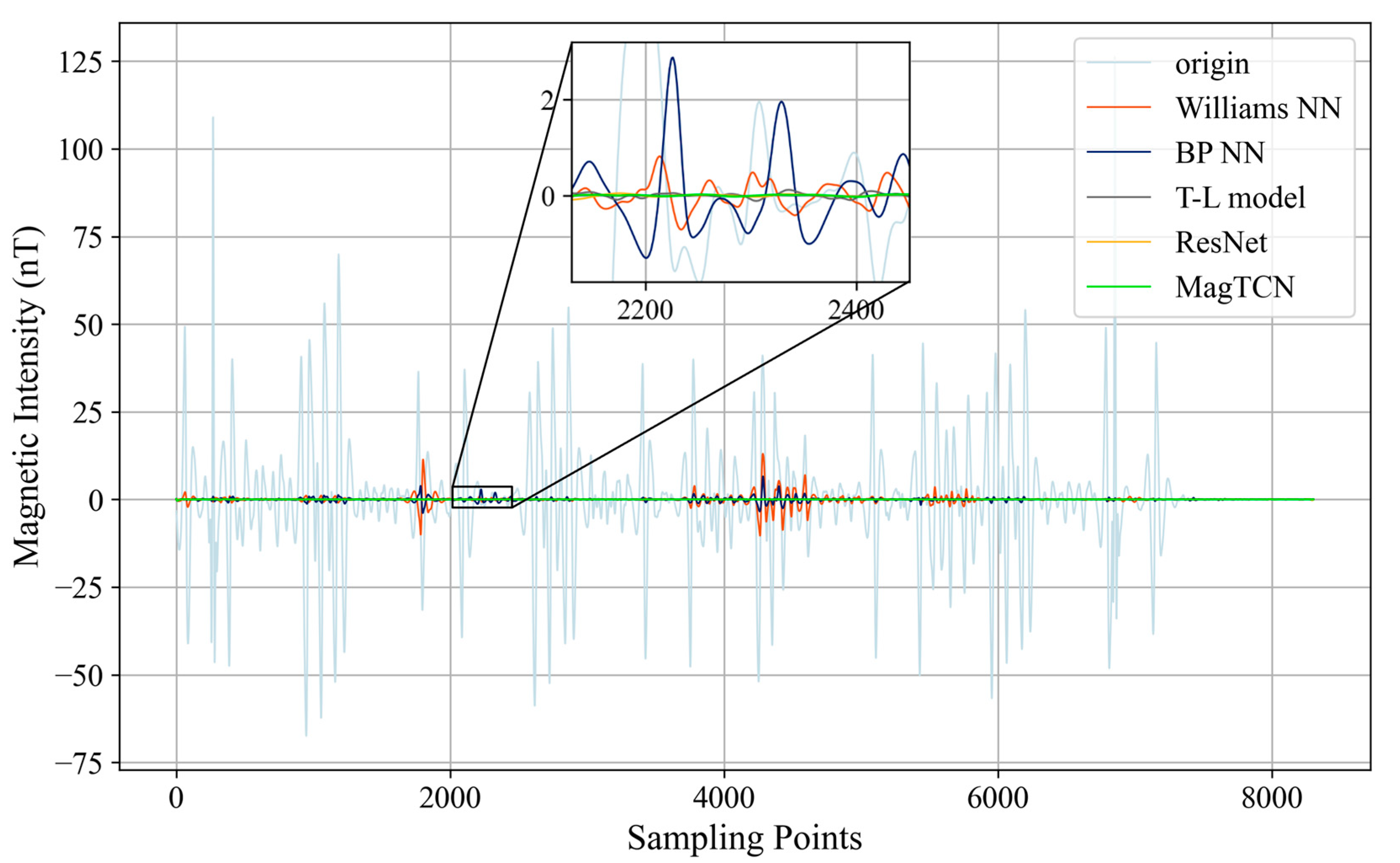
| WilliamsNN | BPNN | ResNet | MagTCN | T–L Model | |
|---|---|---|---|---|---|
| STD (nT) | 1.320 | 0.551 | 0.033 | 0.024 | 0.037 |
| IR | 12.276 | 29.401 | 480.082 | 651.61 | 427.641 |
| Epoch | WilliamsNN Loss | BPNN Loss | ResNet Loss | MagTCN Loss |
|---|---|---|---|---|
| 0 | 136,413.27 | 4169.42 | 3383.46 | 545.77 |
| 50 | 1003.05 | 2757.40 | 547.61 | 48.16 |
| 100 | 827.44 | 634.97 | 381.90 | 24.51 |
| 150 | 581.94 | 498.35 | 369.87 | 19.68 |
| 200 | 301.49 | 366.99 | 288.07 | 11.99 |
| WilliamsNN | BPNN | ResNet | MagTCN | |
|---|---|---|---|---|
| STD (nT) | 1.399 | 1.098 | 0.028 | 0.025 |
| IR | 8.342 | 10.629 | 402.786 | 455.920 |
| WilliamsNN | BPNN | ResNet | MagTCN | |
|---|---|---|---|---|
| STD (nT) | 2.099 | 10.664 | 0.049 | 0.037 |
| IR | 7.298 | 1.436 | 308.679 | 414.090 |
| WilliamsNN | BPNN | ResNet | MagTCN | |
|---|---|---|---|---|
| Average Time Cost (ms) | 0.428 | 0.046 | 1.240 | 1.837 |
| FLOPs (MB) | 0.238 | 0.684 | 105.541 | 95.722 |
Disclaimer/Publisher’s Note: The statements, opinions and data contained in all publications are solely those of the individual author(s) and contributor(s) and not of MDPI and/or the editor(s). MDPI and/or the editor(s) disclaim responsibility for any injury to people or property resulting from any ideas, methods, instructions or products referred to in the content. |
© 2025 by the authors. Licensee MDPI, Basel, Switzerland. This article is an open access article distributed under the terms and conditions of the Creative Commons Attribution (CC BY) license (https://creativecommons.org/licenses/by/4.0/).
Share and Cite
Wang, H.; Zuo, B. An Aeromagnetic Compensation Algorithm Based on a Temporal Convolutional Network. Appl. Sci. 2025, 15, 3105. https://doi.org/10.3390/app15063105
Wang H, Zuo B. An Aeromagnetic Compensation Algorithm Based on a Temporal Convolutional Network. Applied Sciences. 2025; 15(6):3105. https://doi.org/10.3390/app15063105
Chicago/Turabian StyleWang, Han, and Boxin Zuo. 2025. "An Aeromagnetic Compensation Algorithm Based on a Temporal Convolutional Network" Applied Sciences 15, no. 6: 3105. https://doi.org/10.3390/app15063105
APA StyleWang, H., & Zuo, B. (2025). An Aeromagnetic Compensation Algorithm Based on a Temporal Convolutional Network. Applied Sciences, 15(6), 3105. https://doi.org/10.3390/app15063105