
Design and Simulation Optimization for Hydrodynamic Fertilizer Injector Based on Axial-Flow Turbine Structure

 ,
, 

Abstract
1. Introduction
2. Materials and Methods
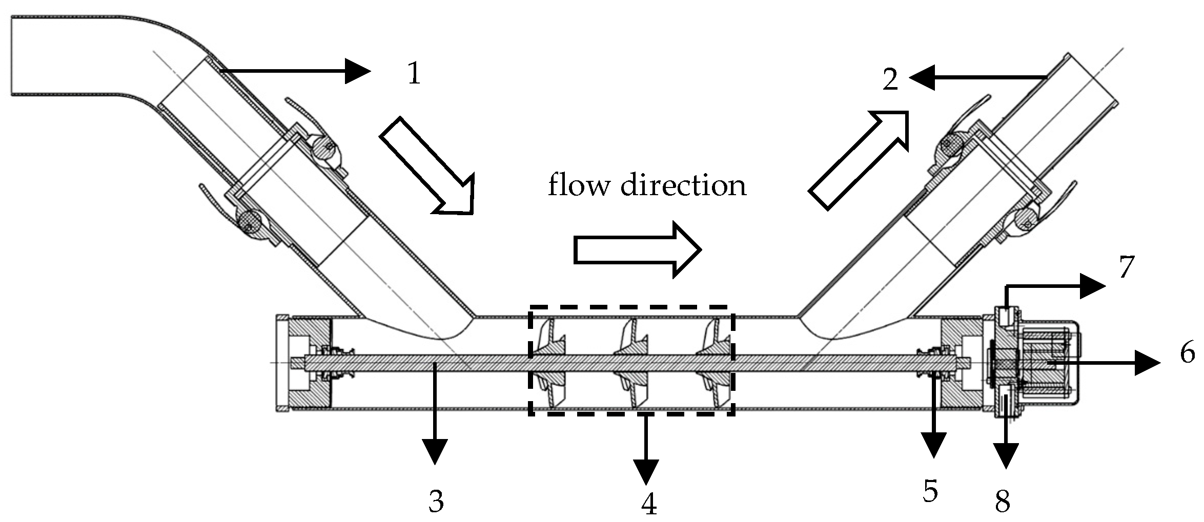
2.1. HFI Design and Working Principle
2.2. Analysis of Parameters Affecting the Hydraulic Performance of the HFI
2.2.1. Experimental Design
2.2.2. Test Methods and Monitoring Indices
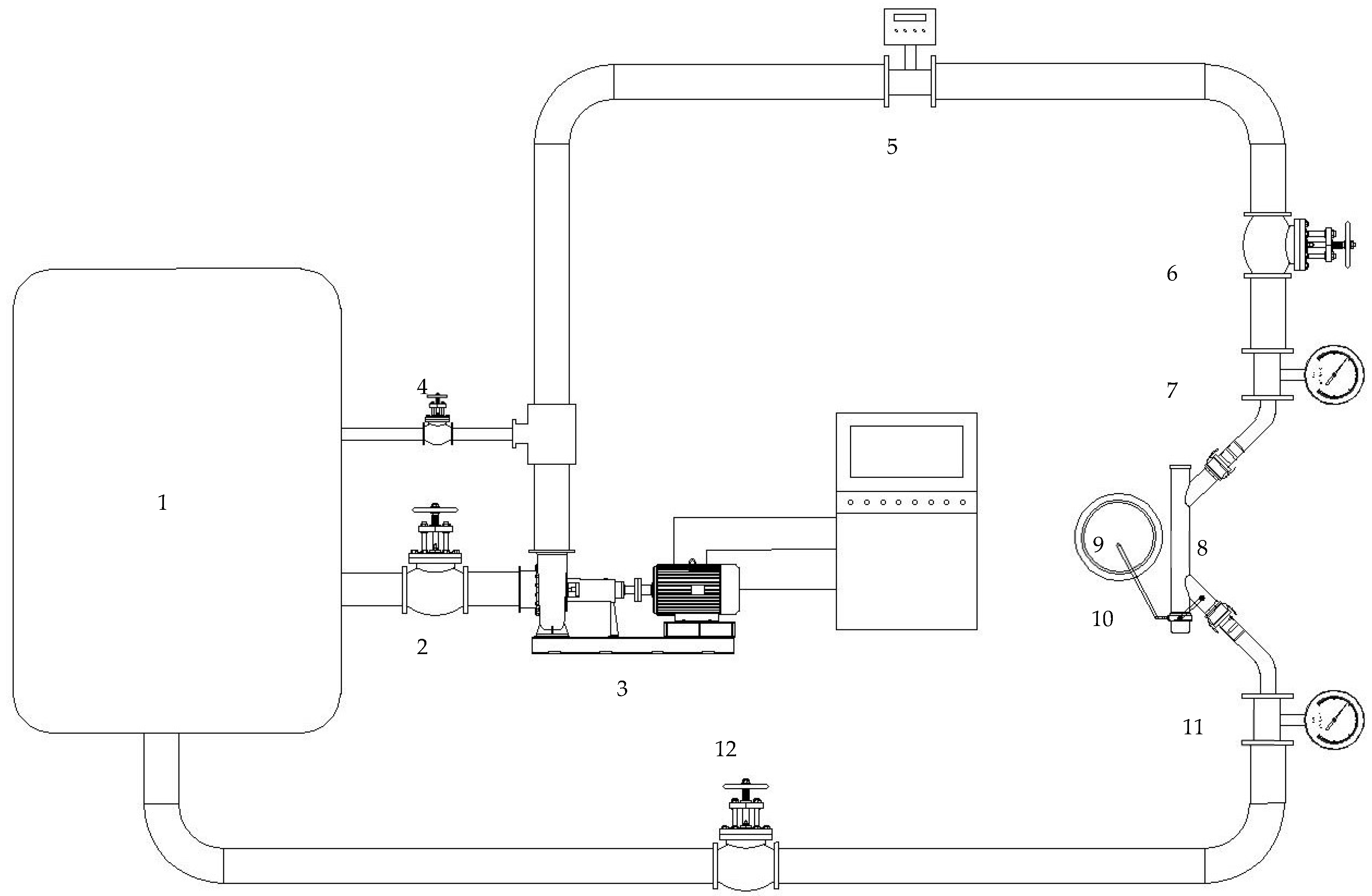
Hydraulic Performance Test
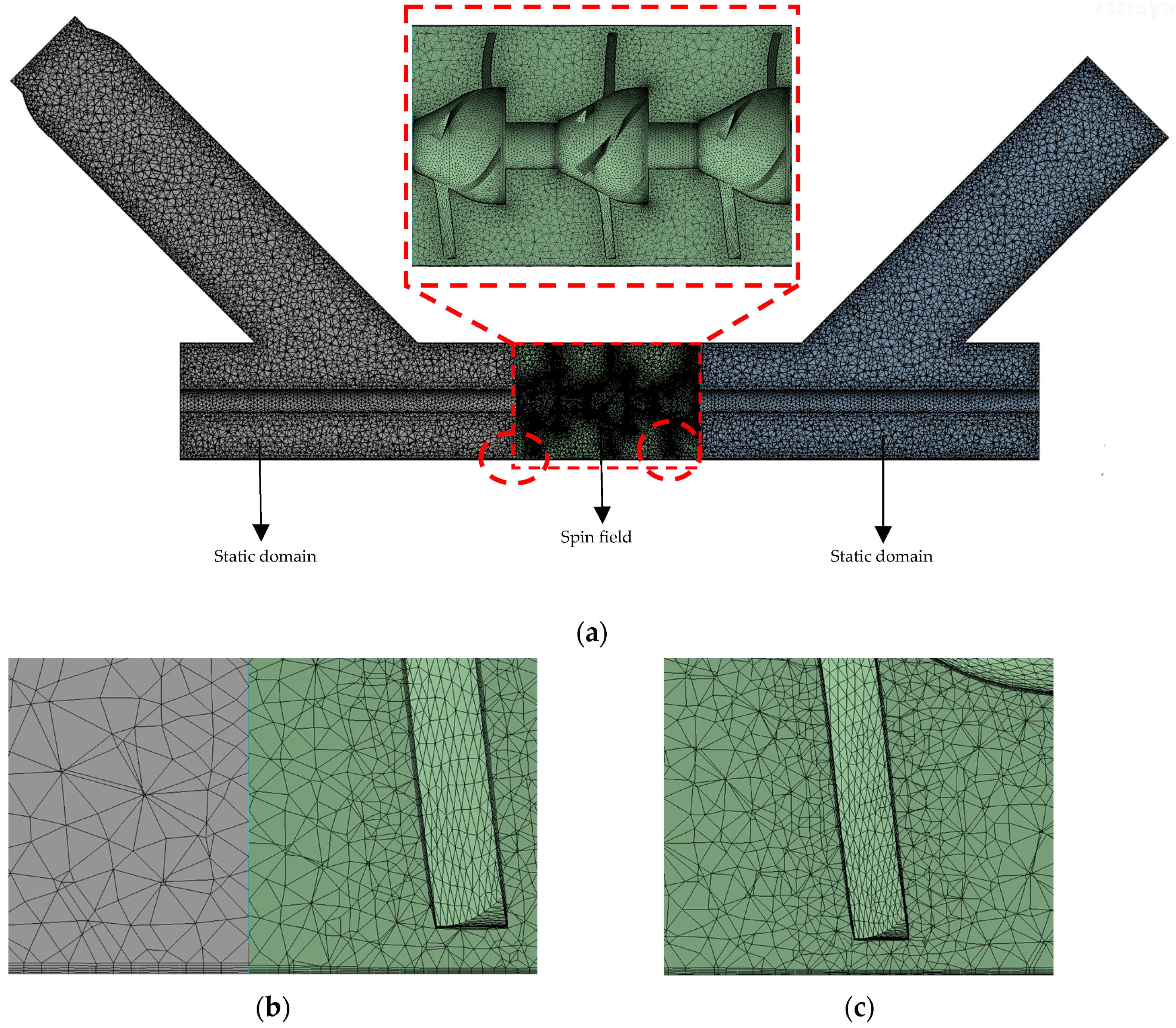
CFD Numerical Simulation of Hydraulic Turbines
2.3. Data Processing
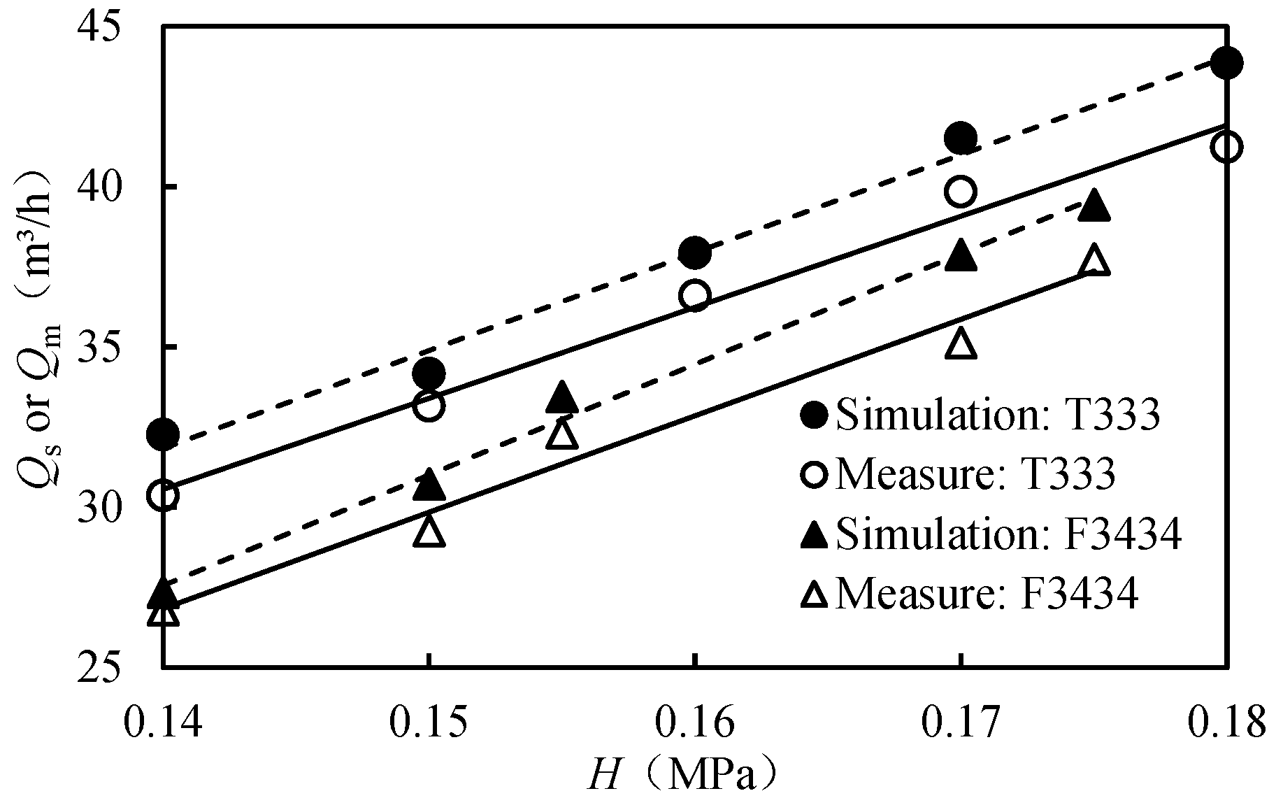
2.3.1. Verification of the CFD Simulation Results
2.3.2. Optimization of the Impeller Structure Parameter Combination
3. Results and Analysis
3.1. Response Law of Outlet Flow and Output Power of AFT to Rotational Speed
3.1.1. Simulation Verification
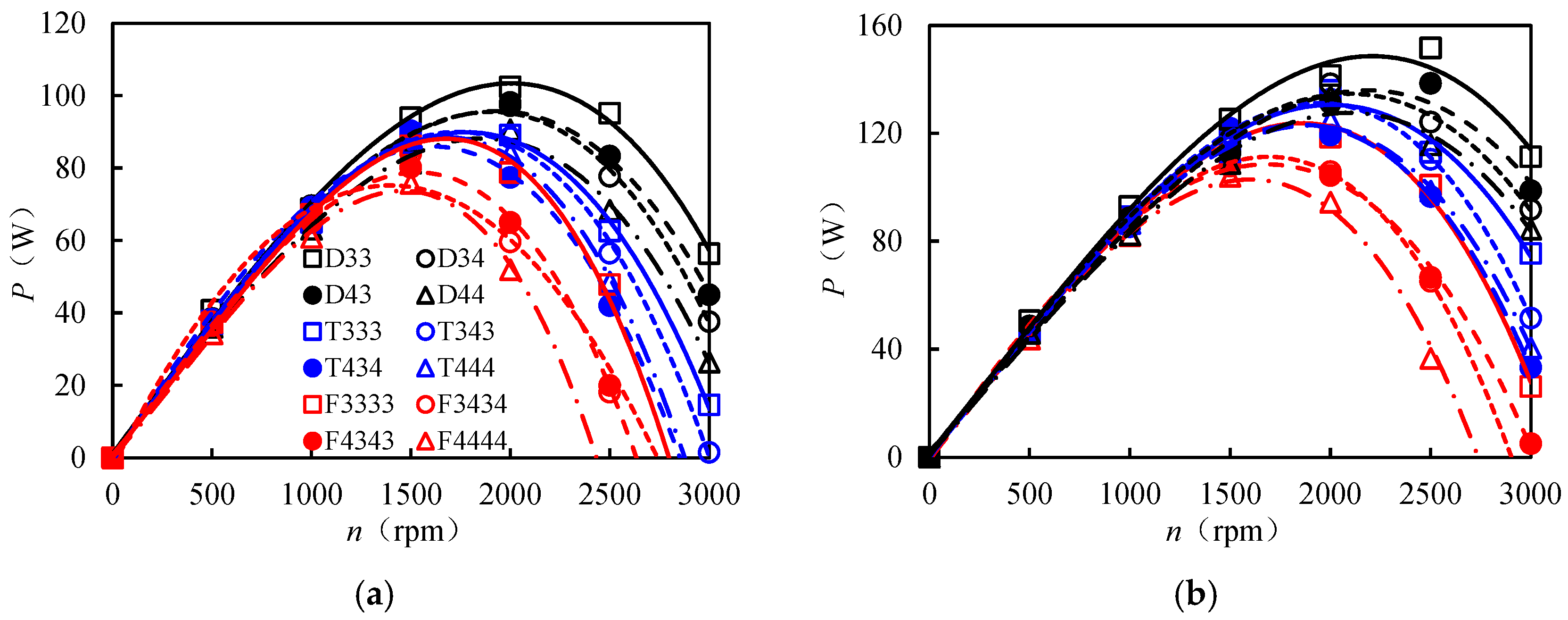
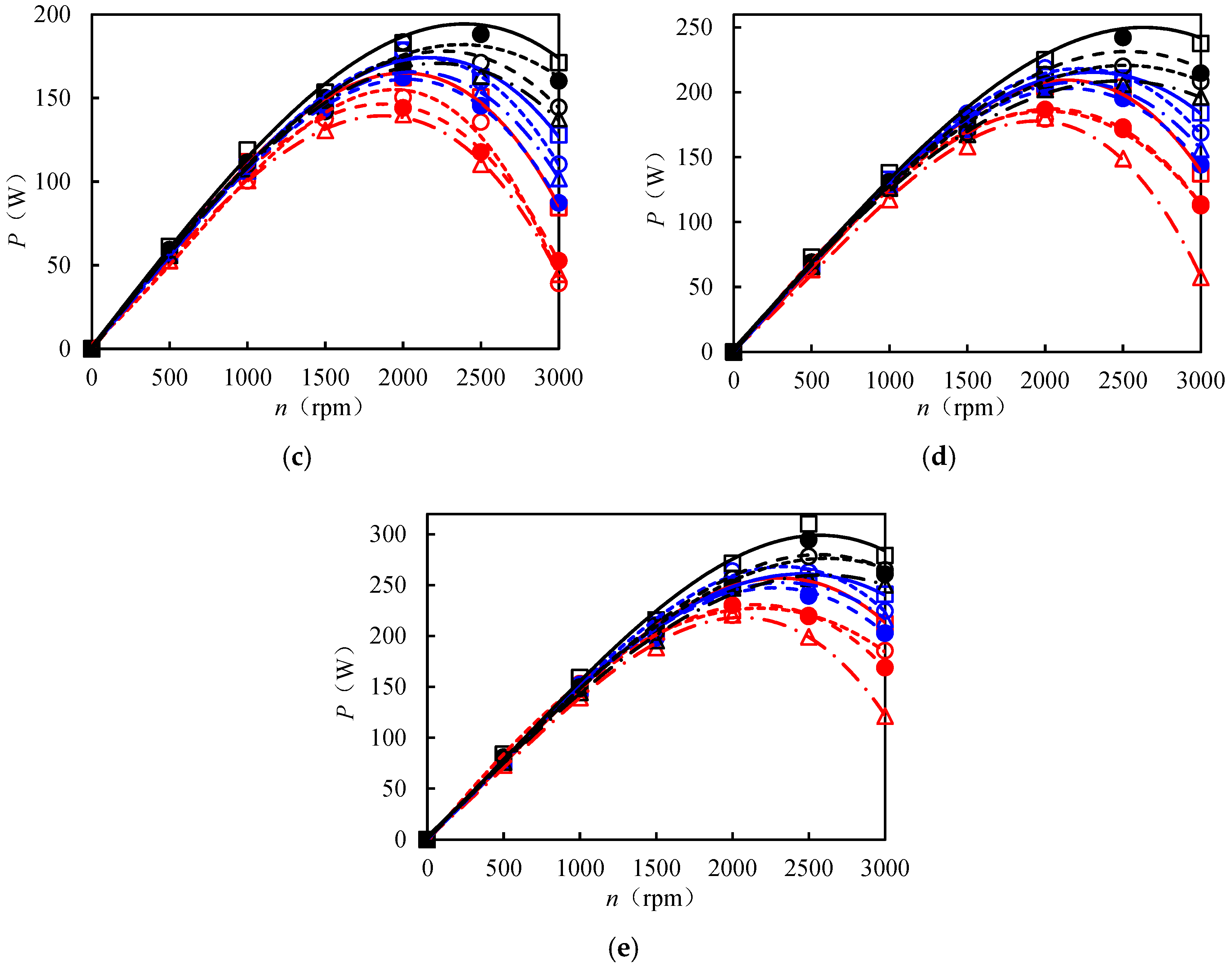
3.1.2. Variation Law of the Output Power of the Axial-Flow Turbine with Rotational Speed
3.2. Internal Flow Field of AFT
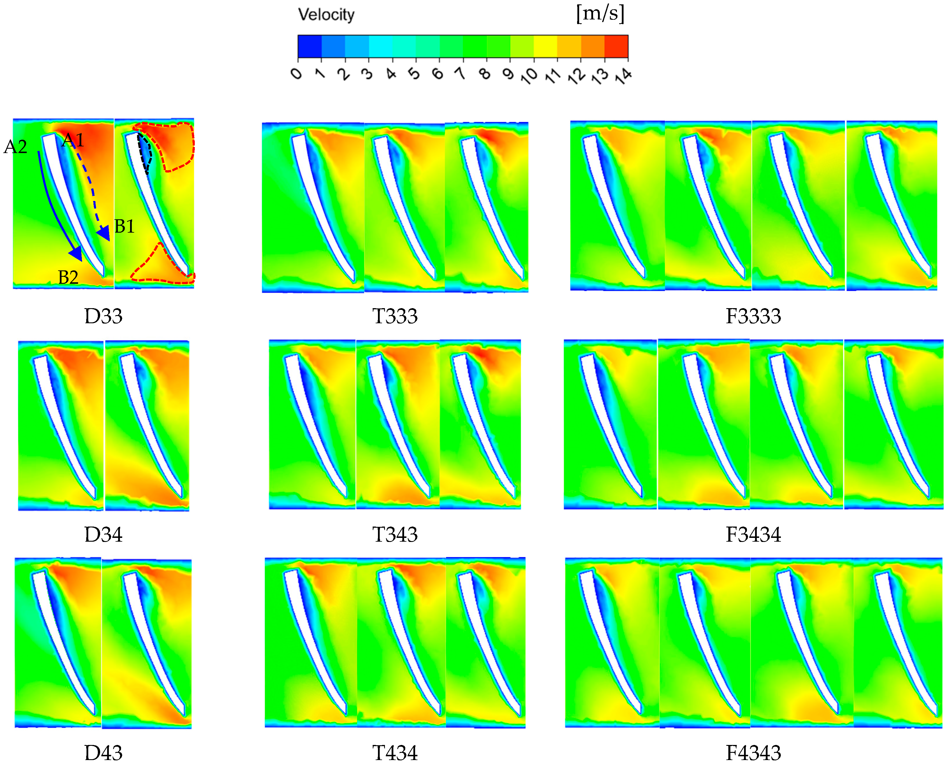
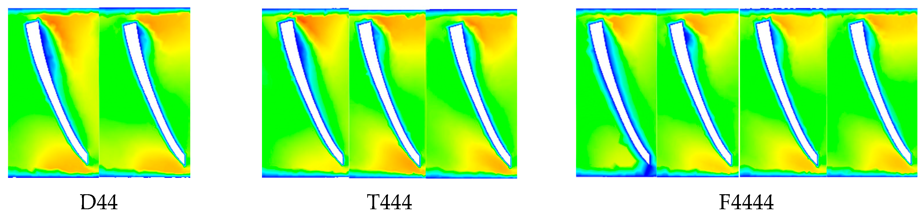
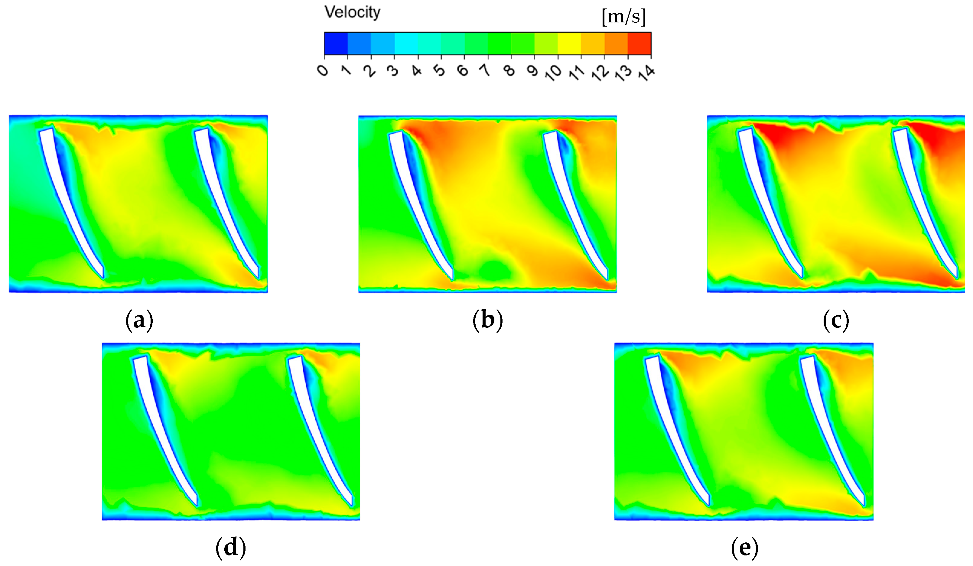
3.2.1. Velocity Cloud Diagram
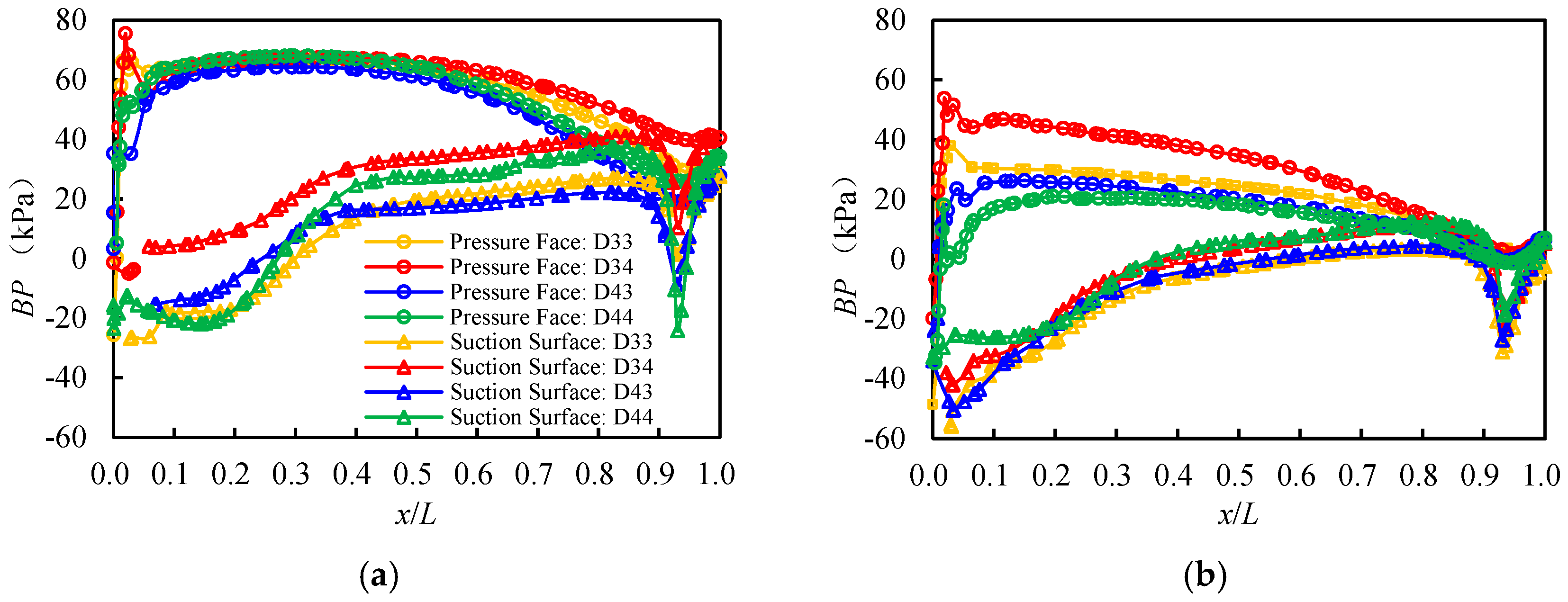
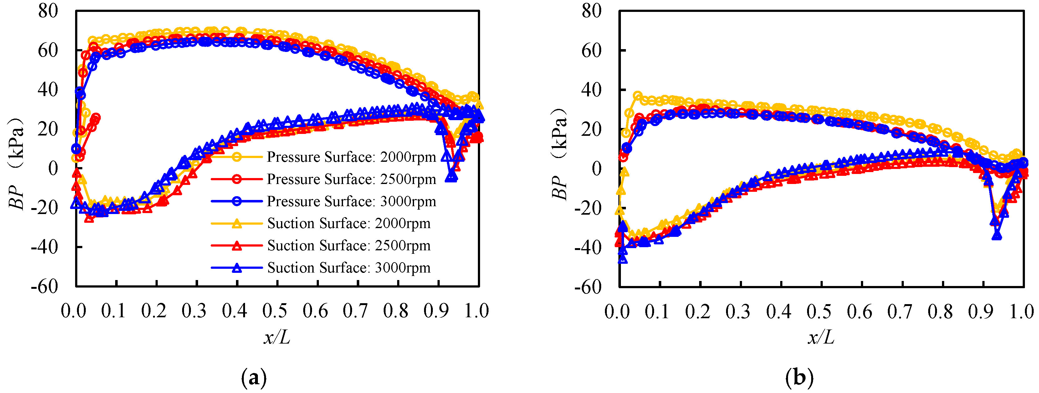
3.2.2. Blade Surface Pressure Curve
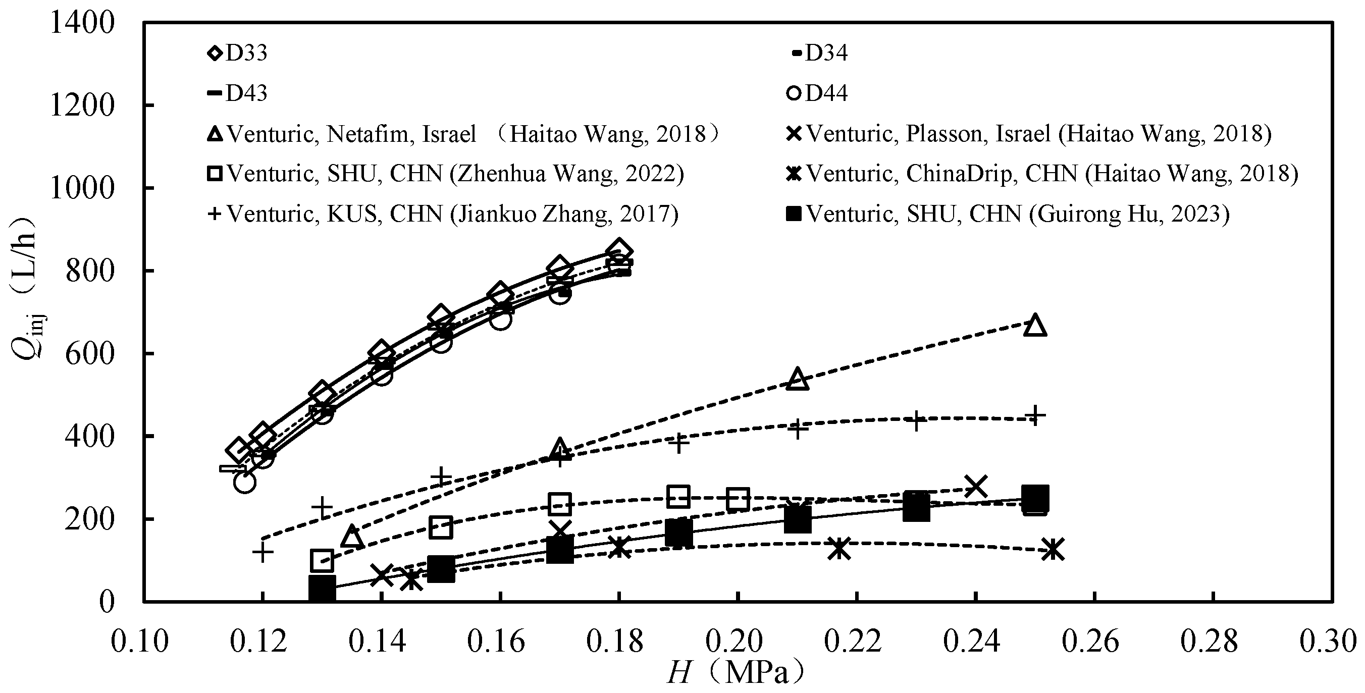
3.3. Fertilization Performance of the Optimized HFI
4. Discussion
4.1. Response Law of AFT Hydraulic Performance to Structural Parameters
4.2. Internal Flow Field and Selection of AFTs
4.3. Response Law of HFI Fertilizer Injection Performance to AFT Structure Design
5. Conclusions
Author Contributions
Funding
Institutional Review Board Statement
Informed Consent Statement
Data Availability Statement
Conflicts of Interest
Abbreviations
| HFI | Hydrodynamic fertilizer injector |
| AFT | Axial-flow water turbine |
| M1 | Number of impellers |
| M2 | Average number of blades of a single impeller |
| M3 | Layout mode |
| P | Output power |
| NP | Leaf negative pressure |
| Qinj | Fertilizer injection flow |
| H | Inlet pressure |
| Qs | Simulated value of outlet flow |
| Qm | The measured value of outlet flow |
| nRMSE | Root mean square error |
| Pmax | Maximum output power |
| NP | Negative pressure value |
| Hout | Outlet pressure |
| Hmin | Minimum inlet pressure |
| N | Number of all leaves on AFT |
| M | Quality of clear water |
| ΔH | Pressure gradient. |
| t | The time required for the water in the fertilizer barrel to be sucked cleanly |
| E | Rate of change |
| n | Revolution speed |
| N | Grid number |
| Δn | Gradient of speed change |
| BP | Blade surface pressure |
| θ | The angle between water flow direction and blade pressure surface |
| x | It is the horizontal distance between the data points on the straight line a1b1 or a2b2 and the leading edge of the blade. |
| L | For the total length of a1b1 |
| T | AFT torque |
| reg-lv | Low-velocity fluid region |
| reg-hv | High-speed fluid region |
| v | Flow velocity |
| ΔBP | BP difference between pressure surface and suction surface |
| Average value of ΔBP | |
| R2 | Correlation coefficient |
References
- Kabirigi, M.; Prakash, S.O.; Prescella, B.V.; Niamwiza, C.; Quintin, S.P.; Mwamjengwa, I.A.; Zhang, C. Fertigation for environmentally friendly fertilizers application: Constraints and opportunities for its application in developing countries. Agric. Sci. 2017, 8, 292. [Google Scholar] [CrossRef]
- Ministry of Water Resources of the People’s Republic of China. China Water Resources Statistical Yearbook in 2021. 2022. Available online: https://data.cnki.net/yearBook/single?id=N2023110278&pinyinCode=YSLTJ (accessed on 24 December 2024).
- Fan, J.; Lu, X.; Gu, S.; Guo, X. Improving nutrient and water use efficiencies using water-drip irrigation and fertilization technology in Northeast China. Agric. Water Manag. 2020, 241, 106352. [Google Scholar] [CrossRef]
- Li, H.; Tang, P.; Chen, C.; Zhang, Z.; Xia, H. Research status and development trend of fertilization equipment used in fertigation in China. J. Drain. Irrig. Mach. Eng. 2021, 39, 200–209. [Google Scholar] [CrossRef]
- Mazzei Injector Company. Performance Data Drawings: Venturi Injectors. 2023. Available online: https://mazzei.net/support/performance-data-drawings/performance-data-drawings-venturi-injectors/ (accessed on 13 March 2023).
- Fan, J.; Wu, L.; Zhang, F.; Yan, S.; Xiang, Y. Evaluation of drip fertigation uniformity affected by injector type, pressure difference and lateral layout. Irrig. Drain. 2017, 66, 520–529. [Google Scholar] [CrossRef]
- Fan, J.; Zhang, F.; Wu, L.; Yan, S.; Xiang, Y. Field evaluation of fertigation uniformity in a drip irrigation system with a pressure differential tank. Trans. Chin. Soc. Agric. Eng. 2016, 32, 96–101. [Google Scholar] [CrossRef]
- Hu, X.; Yan, H.; Chen, X. Calculation method of fertilizer concentration at outlet based on differential pressure tank considering fertilizer dissolution. Trans. Chin. Soc. Agric. Eng. 2020, 36, 99–106. [Google Scholar] [CrossRef]
- Gu, S.; Gao, J.; Deng, Z.; Lü, M.; Liu, J.; Zong, J.; Fan, X. Effects of border irrigation and fertilization timing on soil nitrate nitrogen distribution and winter wheat yield. Trans. Chin. Soc. Agric. Eng. 2020, 36, 134–142. [Google Scholar] [CrossRef]
- Qi, Z.; Gao, Y.; Sun, C.; Ramos, T.B.; Mu, D.; Xun, Y.; Huang, G.; Xu, X. Assessing water-nitrogen use, crop growth and economic benefits for maize in upper Yellow River basin: Feasibility analysis for border and drip irrigation. Agric. Water Manag. 2024, 295, 108771. [Google Scholar] [CrossRef]
- Song, J.; He, W. Optimization design of large-scale irrigation pipe network under the conditions of pump pressure. Yellow River 2016, 38, 145–148. [Google Scholar] [CrossRef]
- Zhang, J.; Li, J. Optimization analysis of the key working parameters of a potato cleaning machine. J. Agric. Mech. Res. 2018, 40, 28–32. [Google Scholar] [CrossRef]
- Zhang, J.; Li, J. Experiment and analysis of Venturi injector fertilizer performance in a low-pressure irrigation system. J. Agric. Mech. Res. 2019, 41, 183–186. [Google Scholar] [CrossRef]
- Wang, H.; Wang, J.; Yang, B.; Mo, Y. Numerical simulation of Venturi injector with non-axis-symmetric structure. J. Drain. Irrig. Mach. Eng. 2018, 36, 1098–1103. [Google Scholar] [CrossRef]
- Wang, Z.; Hu, G.; Liu, N.; Liu, P.; Cao, Y.; Zhang, D. Effects of diffusion section structure on vortex characteristics and fertilizer absorption performance of non-axisymmetric Venturi injector. Trans. Chin. Soc. Agric. Eng. 2022, 38, 61–69. [Google Scholar] [CrossRef]
- Hu, G.; Guan, X.; Li, S.; Liu, N.; Zhang, J.; Yam, P.D.; Zhang, J.; Wang, Z. Structure optimization and fertilizer injection performance analysis of a non-axisymmetric Venturi injector. Irrig. Drain. 2024, 73, 400–414. [Google Scholar] [CrossRef]
- Luo, Z.; Li, H.; Yang, D. Analysis on volumetric efficiency of proportional dosing pumps. China Rural. Water Hydropower 2016, 9, 91–94. [Google Scholar]
- Zhang, Q.; Li, H.; Tang, P.; Sun, C. Improved design and experimental research of the fertilizer suction structure of a valve-regulated proportional fertilization pump. J. Water Resour. Water Eng. 2020, 31, 186–192. [Google Scholar] [CrossRef]
- Ma, L. Hydraulic Fertilizer Applicator. Patent No. CN201020190348.9, 5 January 2011. [Google Scholar]
- Wang, Z.; Wang, Q.; Li, W.; Zhang, J.; Xie, D. A Hydraulic Drive Fertilizer Pump. Patent No. CN201810671578.8, 12 September 2023. [Google Scholar]
- Yu, L.; Qu, M. A Hydrodynamic Pump Drive Device, Hydrodynamic Pump, and Fertilizer Machine. Patent No. CN202320210091.6, 26 September 2023. [Google Scholar]
- Rodríguez-Pérez, A.M.; Rodríguez-González, C.A.; López, R.; Hernández-Torres, J.A.; Caparrós-Mancera, J.J. Water microturbines for sustainable applications: Optimization analysis and experimental validation. Water Resour. Manag. 2024, 38, 1011–1025. [Google Scholar] [CrossRef]
- Chattha, J.A.; Khan, M.S. Experimental study to test an axial flow pump as a turbine and development of performance characteristics for micro-hydro power plant. ASME Power Conf. 2007, 42738, 615–621. [Google Scholar] [CrossRef]
- Chen, J.; Zhang, Z.H.; Wang, G. Shuǐlì Jīxiè [Hydraulic Machinery]; China Water & Power Press: Beijing, China, 2015. [Google Scholar]
- Zhang, R.; Wang, J.; Qian, W.; Geng, L. Optimization of magnetic pump impeller based on blade load curve and internal flow study. Mathematics 2024, 12, 607. [Google Scholar] [CrossRef]
- Betancour, J.; Velásquez, L.; Rubio Clemente, A.; Chica, E. Performance simulation of water turbines by using 6-DoF UDF and sliding mesh methods. J. Appl. Res. Technol. 2023, 21, 181–195. [Google Scholar] [CrossRef]
- Abbas, A.I.; Qandil, M.D.; Al-Haddad, M.; Amano, R.S. Investigation of horizontal micro Kaplan hydro turbine performance using multi-disciplinary design optimization. J. Energy Resour. Technol. 2020, 142, 5. [Google Scholar] [CrossRef]
- Wang, X.; Zhang, X.; Miao, S.; Bai, X. Hydraulic performance experiment and numerical simulation of a hydraulic turbine at different speeds. Water Resour. Power 2024, 42, 186–190. [Google Scholar] [CrossRef]
- Janjua, A.B.; Khalil, M.S.; Saeed, M. Blade profile optimization of Kaplan turbine using CFD analysis. Mehran Univ. Res. J. Eng. Technol. 2013, 32, 559–574. Available online: https://www.researchgate.net/publication/352708109_Blade_Profile_Optimization_of_Kaplan_Turbine_Using_CFD_Analysis (accessed on 24 December 2024).
- Yang, S.S.; Kong, F.Y.; Qu, X.Y.; Jiang, W.M. Influence of blade number on the performance and pressure pulsations in a pump used as a turbine. J. Fluids Eng. 2012, 134, 124503. [Google Scholar] [CrossRef]
- Ji, Y.; Yang, Z.; Ran, J.; Li, H. Multi-objective parameter optimization of turbine impeller based on RBF neural network and NSGA-II genetic algorithm. Energy Rep. 2021, 7, 584–593. [Google Scholar] [CrossRef]
- Derakhshan, S.; Kasaeian, N. Optimization, numerical, and experimental study of a propeller pump as turbine. J. Energy Resour. Technol. 2014, 136, 012005. [Google Scholar] [CrossRef]
- Mo, Y.; Zhao, C.; Zhang, B.; Zhang, Y.; Gong, S.; Jiao, X.; Gong, Y.; Lin, J.; Zhang, X. Low-Pressure Pipeline Water Conveyance Irrigation Hydrodynamic Fertilization. Device. Patent No. CN202410441384.4, 9 August 2024. [Google Scholar]
- Liu, C. (Ed.) Pumps and Pump Stations; China Water & Power Press: Beijing, China, 2009. [Google Scholar]
- Ohiemi, I.E.; Sunsheng, Y.; Singh, P.; Li, Y.; Osman, F. Evaluation of energy loss in a low-head axial flow turbine under different blade numbers using entropy production method. Energy 2023, 274, 127262. [Google Scholar] [CrossRef]
- Wang, S.; Ma, C.; Zhang, C. Optimization of residual pressure turbine impeller in oilfield water injection pipeline based on Fluent. Manuf. Autom. 2023, 45, 144–148. [Google Scholar] [CrossRef]
- Wu, H.; Feng, J.; Wu, G.; Guo, P.; Luo, X. The blade geometry modification and performance research for bulb turbine based on CFD. J. Xi’an Univ. Technol. 2013, 29, 290–294. [Google Scholar] [CrossRef]
- Park, J.H.; Lee, N.J.; Wata, J.V.; Hwang, Y.C.; Kim, Y.T.; Lee, Y.H. Analysis of a pico tubular-type hydro turbine performance by runner blade shape using CFD. IOP Conf. Ser. Earth Environ. Sci. 2012, 15, 042031. [Google Scholar] [CrossRef]
- Yang, S.; Fang, T.; Zhou, C.; Zhao, E.; Wang, T. Influence of axial spacing on hydraulic performance of tubular turbine. J. Drainage Irrig. Mach. Eng. 2023, 41, 338–345. [Google Scholar] [CrossRef]
- GB/T 19792-2012; Agricultural Irrigation Equipment Hydraulic Chemical Fertilizer-Pesticide Injection Pumps. National Agricultural Machinery Standardization Technical Committee: Beijing, China, 2013.
- Muis, A.; Sutikno, P.; Soewono, A.; Hartono, F. Design optimization of axial hydraulic turbine for very low head application. Energy Procedia 2015, 68, 263–273. [Google Scholar] [CrossRef]
- Hoghooghi, H.; Durali, M.; Kashef, A. A new low-cost swirler for axial micro hydro turbines of low head potential. Renew. Energy 2018, 128, 375–390. [Google Scholar] [CrossRef]
- Wang, H.; Chen, Y.; Wang, J.; Yang, B.; Mo, Y. Experimental study on comprehensive working performance of Venturi injector. J. Drainage Irrig. Mach. Eng. 2018, 36, 340–346. [Google Scholar] [CrossRef]
- Nishi, Y.; Kobori, T.; Mori, N.; Inagaki, T.; Kikuchi, N. Study of the internal flow structure of an ultra-small axial flow hydraulic turbine. Renew. Energy 2019, 139, 1000–1011. [Google Scholar] [CrossRef]
- Wang, S.; Gong, F.; Li, Z. Optimization design and experimental study of hydraulic turbine based on residual pressure power generation system. J. Mach. Des. 2022, 39, 77–83. [Google Scholar] [CrossRef]
- Wang, S.; Li, M.; Li, Z. Influence of impeller stage on hydrodynamic performance of a tidal turbine. Ship Eng. 2020, 42, 23–28. [Google Scholar] [CrossRef]
- Zhao, Z.; He, J.; Wang, C. Hydraulics, 3rd ed.; Tsinghua University Press: Beijing, China, 2021. [Google Scholar]
- Fang, T. Numerical Calculation and Experimental Study of Micro Shaft-Extension Axial Turbine. Master’s Thesis, Jiangsu University, Zhenjiang, China, 2022. [Google Scholar] [CrossRef]
- Miao, S.; Wu, H.; Wang, X.; Shi, F.; Yang, J. Research on internal energy loss mechanism of axial pump as turbine based on entropy production theory. J. Xihua Univ. Nat. Sci. Ed. 2023, 42, 1–9. Available online: http://kns.cnki.net/kcms/detail/51.1686.N.20240528.0924.002.html (accessed on 24 December 2024).
- Guo, Y.; Yang, C.; Mo, Y.; Wang, Y.; Lv, T.; Zhao, S. Numerical study on the mechanism of fluid energy transfer in an axial flow pump impeller under the rotating coordinate system. Front. Energy Res. 2023, 10, 1106789. [Google Scholar] [CrossRef]
- Kan, K.; Binama, M.; Chen, H.; Zheng, Y.; Zhou, D.; Su, W.; Muhirwa, A. Pump as turbine cavitation performance for both conventional and reverse operating modes: A review. Renew. Sustain. Energy Rev. 2022, 168, 112786. [Google Scholar] [CrossRef]
- Wu, R.; Liu, H.; Chen, W.; Ji, S.; Cao, L.; Wu, D. Experimental investigation of propeller blade back cavitation induced pressure pulses by synchronous observation. Ocean Eng. 2024, 298, 116971. [Google Scholar] [CrossRef]
- Ren, L.; Zhang, H.; Zhang, S.; Fan, G.; Li, Y.; Song, Y. Experimental research on efficient irrigation system with mixed fertilizer in integration of water and fertilizer. J. Phys. Conf. Ser. 2020, 1550, 042004. [Google Scholar] [CrossRef]
- Wang, H.; Wang, J.; Yang, B.; Mo, Y.; Zhang, Y.; Ma, X. Simulation and optimization of Venturi injector by machine learning algorithms. J. Irrig. Drain. Eng. 2020, 146, 04020021. [Google Scholar] [CrossRef]
- García-Saldaña, M.D.; Castañeda-Chávez, A.; Pérez-Vázquez, J.P.; Martínez-Dávila, E.; Carrillo-Ávila, E. Design of venturi-type fertilizer injectors to low-pressure irrigation systems. J. Agric. Sci. 2023, 15, 25. [Google Scholar] [CrossRef]
- Shi, Y.; Hu, Z.; Wang, X.; Odhiambo, M.O.; Sun, G. Fertilization strategy and application model using a centrifugal variable-rate fertilizer spreader. Int. J. Agric. Biol. Eng. 2018, 11, 41–48. Available online: https://www.ijabe.org/index.php/ijabe/article/view/3789 (accessed on 24 December 2024). [CrossRef]


| Experimental Treatment | Number of Impellers (M1) (Units) | Total Number of Leaves (N) (Pieces) | Average Blade of a Single Impeller | Layout Mode (M3) | Structural Design Drawing | |
|---|---|---|---|---|---|---|
| Quantity (M2) (Sheet) | Grouping | |||||
| D33 | 2 | 6 | 3.0 | Little | Same: 3 + 3 |  |
| D34 | 7 | 3.5 | Median | Less-more: 3 + 4 |  | |
| D43 | 7 | 3.5 | Median | More-less: 4 + 3 |  | |
| D44 | 8 | 4.0 | Multiplicity | Same: 4 + 4 | 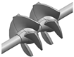 | |
| T333 | 3 | 9 | 3.0 | Little | Same: 3 + 3 + 3 |  |
| T343 | 10 | 3.3 | Median | Less-more: 3 + 4 + 3 |  | |
| T434 | 11 | 3.7 | Median | More-less: 4 + 3 + 4 |  | |
| T444 | 12 | 4.0 | Multiplicity | Same: 4 + 4 + 4 | 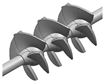 | |
| F3333 | 4 | 12 | 3.0 | Little | Same: 3 + 3 + 3 + 3 | 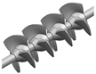 |
| F3434 | 14 | 3.5 | Median | Less-more: 3 + 4 + 3 + 4 |  | |
| F4343 | 14 | 3.5 | Median | More-less: 4 + 3 + 4 + 3 | 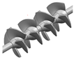 | |
| F4444 | 16 | 4.0 | Multiplicity | Same: 4 + 4 + 4 + 4 | 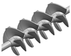 | |
| Experimental Treatment | Pmax (W) | |||||
|---|---|---|---|---|---|---|
| H = 0.14 MPa | H = 0.15 MPa | H = 0.16 MPa | H = 0.17 MPa | H = 0.18 MPa | Ave | |
| D33 | 102.37 | 151.61 | 201.29 | 260.18 | 310.10 | 201.43 |
| D34 | 98.07 | 138.27 | 183.43 | 219.88 | 278.18 | 179.80 |
| D43 | 97.20 | 138.49 | 188.09 | 242.25 | 294.56 | 188.71 |
| D44 | 90.60 | 133.66 | 176.24 | 212.35 | 256.66 | 170.94 |
| Mean | 79.80 b | 140.51 a | 187.76 a | 233.66 a | 284.88 a | 185.22 a |
| T333 | 89.42 | 135.85 | 178.42 | 212.18 | 258.09 | 174.79 |
| T343 | 90.24 | 132.63 | 178.20 | 218.59 | 262.88 | 176.51 |
| T434 | 89.70 | 121.90 | 162.32 | 203.37 | 239.37 | 163.33 |
| T444 | 86.80 | 124.89 | 165.84 | 206.57 | 250.43 | 166.91 |
| Mean | 89.04 a | 128.82 b | 171.20 b | 210.18 b | 252.69 ab | 170.38 a |
| F3333 | 86.09 | 118.51 | 162.21 | 203.92 | 257.51 | 165.65 |
| F3434 | 79.25 | 107.75 | 150.43 | 193.64 | 219.27 | 150.07 |
| F4343 | 80.17 | 109.60 | 144.07 | 186.68 | 219.86 | 148.08 |
| F4444 | 75.81 | 104.14 | 140.18 | 180.25 | 199.24 | 139.92 |
| Mean | 80.33 b | 110.00 c | 149.22 c | 191.12 b | 223.97 b | 150.93 b |
| F value for M1 | 18.979 | 43.87 | 24.82 | 12.93 | 22.86 | 24.39 |
| Sig-M1 | ** | * | * | * | * | * |
| F value for M2 | 0.78 | 8.74 | 5.91 | 3.85 | 8.77 | 8.16 |
| Sig-M2 | NS | NS | NS | NS | NS | NS |
| F value for M1 × M2 | 16.19 | 0.17 | 0.21 | 0.91 | 1.55 | 0.85 |
| Sig-M1 × M2 | NS | NS | NS | NS | NS | NS |
Disclaimer/Publisher’s Note: The statements, opinions and data contained in all publications are solely those of the individual author(s) and contributor(s) and not of MDPI and/or the editor(s). MDPI and/or the editor(s) disclaim responsibility for any injury to people or property resulting from any ideas, methods, instructions or products referred to in the content. |
© 2025 by the authors. Licensee MDPI, Basel, Switzerland. This article is an open access article distributed under the terms and conditions of the Creative Commons Attribution (CC BY) license (https://creativecommons.org/licenses/by/4.0/).
Share and Cite
Zhao, C.; Mo, Y.; Zhang, B.; Liu, S.; Zhang, Q.; Xiao, J.; Gong, Y. Design and Simulation Optimization for Hydrodynamic Fertilizer Injector Based on Axial-Flow Turbine Structure. Appl. Sci. 2025, 15, 2963. https://doi.org/10.3390/app15062963
Zhao C, Mo Y, Zhang B, Liu S, Zhang Q, Xiao J, Gong Y. Design and Simulation Optimization for Hydrodynamic Fertilizer Injector Based on Axial-Flow Turbine Structure. Applied Sciences. 2025; 15(6):2963. https://doi.org/10.3390/app15062963
Chicago/Turabian StyleZhao, Chunlong, Yan Mo, Baozhong Zhang, Shuhui Liu, Qi Zhang, Juan Xiao, and Yiteng Gong. 2025. "Design and Simulation Optimization for Hydrodynamic Fertilizer Injector Based on Axial-Flow Turbine Structure" Applied Sciences 15, no. 6: 2963. https://doi.org/10.3390/app15062963
APA StyleZhao, C., Mo, Y., Zhang, B., Liu, S., Zhang, Q., Xiao, J., & Gong, Y. (2025). Design and Simulation Optimization for Hydrodynamic Fertilizer Injector Based on Axial-Flow Turbine Structure. Applied Sciences, 15(6), 2963. https://doi.org/10.3390/app15062963