Susceptibility and Remanent Magnetization Estimates from Orientation Tools in Borehole Imaging Logs

Abstract

Orientation tools in borehole imaging logs acquire magnetic information that is currently used for spatial and geographical orientation of the images. We propose to use this magnetic field information to estimate both magnetic susceptibility and remanent magnetization of rocks inside wells. Measurements of these magnetic parameters are not often available in hydrocarbon exploration to support forward modeling of magnetic data, an interpretation tool that has played important role in the exploration risk reduction in the Pre-Salt prospects of Campos Basin, Brazil. The acquired magnetic data requires corrections for tool rotation and diurnal variation of the Earth’s magnetic field before calculation. Then, using a set of simple equations and reasonable assumptions we were able to estimate the magnetic susceptibility of carbonates and basalts, as well as the remanent magnetization of the basalts, from a Pre-Salt well in Campos Basin. When compared to susceptibility values measured in laboratory for the same rock interval, our results show a significant match. This promising result shows the importance of our methodology in providing reliable information that can minimize uncertainties in forward modeling of magnetic data, which contributes to reduction of hydrocarbon exploration risks. Given that direct susceptibility and remanence measurements require oriented samples, a complex and expensive operation in wells, our results offer this rock information without any extra costs since imaging logs are commonly acquired in exploration wells. Besides its use in hydrocarbon exploration, our methodology can be applied to mineral exploration where magnetic susceptibility is an important property for rock identification.

1. Introduction

Borehole imaging tools, like the Formation Micro-Imaging (FMI), for instance, carry triaxial magnetometers in an auxiliary orientation tool (also known as inclinometers) that acquire magnetic information used for spatial and geographical orientation of the images. Until recently, the use of the magnetic data acquired by these orientation tools was restricted to support the inclinometry data. According to [1], the perception that changes in the measured magnetic field were caused by the presence of magnetic rocks in the borehole has extended the use of this data to help identifying igneous rock intervals during analysis of imaging tools data. The fact that these magnetic data can detect the presence of igneous rocks rises the question if they are sensitive enough to allow estimates of some magnetic properties of these rocks, more specifically, the magnetic susceptibility.

Interpretation of magnetic data is traditionally used in petroleum exploration to map the geological distribution of magnetic rocks in subsurface. Among various interpretation techniques, the forward modeling of magnetic data is a typical approach for estimation of positions, depths, geometries and magnetic properties of the rocks in exploration areas. In general, the forward modeling technique searches for a reliable geological solution that fits the magnetic anomaly observed in the survey area. This interpretation process is mainly ruled by two variables: the geometry of the rocks and their magnetic susceptibility. Well data and other geophysical data, like seismic and gravity for instance, may provide the necessary control to the source’s geometry variability, while measurements of magnetic susceptibility are rare specially in oil industry.

Forward modeling has played important role to the exploration of Pre-Salt prospects in offshore Brazil, where it has been used to help in the differentiation between carbonates and igneous rocks, whose distinction in seismic images are often difficult. Examples of such use can be found in [2], who discussed the utility and problems encountered when modeling in Santos Basin, offshore Brazil. Figure 1 shows a representative example from [2]. In both Figure 1a,b, the upper panels show the magnetic profiles where the blue dotted line represent the observed data, the continuous blue line is the data calculated from the model and the continuous red line accounts for the misfit. The models are shown in the lower panels where the blue region are the non-magnetic rocks (carbonates and other sedimentary rocks) while the pink regions represent the igneous rocks, whose magnetic susceptibility comes from literature values due to the absent of measurements. The green lines are the interface between the layers as interpreted from seismic data. The initial interpretation (Figure 1a) suggested the presence a thicker and shallower igneous package at the top of the structure. The modeling solution (exhibited in Figure 1b) shows that a thinner and deeper igneous package fits better the observed data and, therefore, should be more likely to be true [2]. Latter drilling has proved that the model proposed by the forward modeling was correct.

The importance of magnetic forward modeling to Pre-Salt exploration, specially where seismic interpretation is ambiguous, contrasts with the lack of susceptibility measurements in boreholes. Since magnetic susceptibility in rocks may vary in orders of magnitude, the use of literature values may not always provide reliable results. Estimates from borehole magnetic data collected in nearby wells may provide the necessary control for the forward modeling. The incorporation of more reliable magnetic susceptibility estimates into these models would make them more realistic contributing for exploration risks reduction.

Despite its utility for magnetic modeling, the development of tools for borehole magnetic susceptibility measurements was greatly driven by the magnetostratigraphy due to its application in determining the absolute age of geological formations. Examples of interpretation of magnetic logging data in sediments can be found in [3,4] who have studied the magnitude and variations of magnetic susceptibility in sedimentary and volcanoclastic rocks to understand their influence on induction logs.

Magnetic well logging tools have been developed by both oil and service companies since the middle of last century. Two magnetic well logging instruments capable of acquiring magnetic susceptibility as well as the total magnetic field were developed by Magnolia Petroleum according to [5]. The development of the GHMT (Geological High Sensibility Magnetic Tool) by Total with the help of Schlumberger was described by [6,7]. The GHMT is a magnetic logging tool developed for recording the total magnetic field and the magnetic susceptibility of rocks in oil wells. Besides oil companies, the mineral industry was also researching borehole magnetic susceptibility tools. A magnetic susceptibility log system for uranium exploration whose development was supported by the Department of Energy of United States was described by [8,9]. The basic theory and results of an inductive magnetic susceptibility logger (Geonics EM39S) for shallow lithological applications was presented by [10] who have used it to study unconsolidated sediments and rocks in Canada. A magnetic tensor gradiometer, developed by [11] in Australia for iron ore exploration, is an instrument capable to measure magnetic field gradients in all directions within a borehole, however it does not provide susceptibility measurements.

Alternatively, methods of getting indirect measurements of the magnetic susceptibility of rocks have been proposed as well. Such methods were based mainly on changes in acquisition methodology, choice of parameters and data processing of induction and NMR (Nuclear Magnetic Resonance) tools. The use of induction logs to determine relative magnetic susceptibility with focus on the perturbations in induction results caused by the magnetic formations was proposed by [12]. Apparent magnetic susceptibility contrast estimates between rock and a saturating liquid was performed by [13] from measures of the free induction decay in core plugs, powdered rocks and drilled cuttings, but not in well logs.

The developments and applications of the logging magnetic tools have yielded promising results. Examples of the application of borehole magnetic susceptibility studies in different fields can be found in [14], who evaluates the use of high-resolution magnetic susceptibility logs to characterize climate-forced sedimentation evolution and in [15] who has used high-sensitivity induction magnetic susceptibility probe to infer mineralogical changes and lithology variations in shallow mapping applied to groundwater studies. Environmental studies has also made use of magnetic susceptibility to identify variations in sediment composition as in [16], but in most of the cases, the logging is carried out on a core instead of inside the borehole. Magnetic susceptibility logs are also common in ocean drilling programs, as in [17] for instance, but they usually log cores of recovered sediments and do not take borehole measurements. The use of magnetic susceptibility downhole finds applicability even in archaeology, as in [18] who reviews the role of magnetic susceptibility in archaeogeophysical studies.

Despite of the large applicability of magnetic susceptibility for sediment studies, little application of borehole magnetic logging have emerged in oil exploration industry. Even though [19] provides an extensive review of magnetic susceptibility measurements applications for reservoir characterization, most of the discussed results were based on laboratory rather than logging measurements. As a consequence, to our knowledge, this type of borehole logging tools can not be found for commercial use in oil industry nowadays. In this paper we propose to overcome this lack of direct measurements by estimating the magnetic susceptibility of the rocks along the borehole using the magnetic data acquired by the magnetometer included in the orientation tools of imaging logs.

2. Materials and Methods

The total field F measured inside a borehole can be related to the Earth’s magnetic field H and to the total magnetization $M_T$ of a rock as:

$$F=\left(H+M_T\right)=H+\left(M_H+M_R\right)=H+\left(\chi H+M_R\right),$$

(1)

where $M_H$ is the component of magnetization produced in response to the Earth’s magnetic field, $M_R$ is the natural remanent magnetization and $\chi$ is the rock’s magnetic susceptibility. The natural remanent magnetization is a permanent magnetization that remains in the rock even in the absence of an inducing field, recording its magnetization history. The magnetic susceptibility is a dimensionless physical property of the rock that in cases of sufficiently weak fields, like the Earth’s magnetic field, represents a constant of proportionality relating the induced magnetization and the applied field. Since the induced magnetization is essentially parallel to the applied field, the magnetic susceptibility is a scalar quantity for most of rocks. Equation (1) is of fundamental importance because it represents the basis for all estimates carried in this study.

As Equation (1) is a vector sum, it can only be correctly done with the knowledge of the three parameters that describe a magnetic field vector: magnitude F, inclination I and declination D. Alternatively, the sum can be simplified by decomposing each vector in its components in the x-, y- and z-directions as defined in Figure 2a. However, the triaxial magnetometers used in image logs to determine tool orientation and/or well direction measure the three components of the magnetic field F with respect to the tool coordinate system instead of true geographic coordinate system. In order to correctly perform the vector sum in Equation (1) it is necessary to project the field components from the tool’s system into the geographic system described in Figure 2a.

In the tool orientation system, the x-axis points to the direction of a reference marker, called P1 or Pad #1, located in the plane perpendicular to the z-axis, which for vertical wells correspond to the borehole axis (Figure 2b). As the tool rotates during logging operations, the tool’s x-axis points not to north as defined in Figure 2a, but to different directions. Consequently, the magnitude of acquired horizontal components do not represent the true amplitude in north and east direction. Figure 3a shows the magnetic field acquired in a typical well as an example of the variation in amplitude of the horizontal components caused by the tool’s rotation. The strong fluctuations occurring in the horizontal components of the acquired magnetic field need to be corrected before calculations.

According to [20] the orientation of the tool in the geographical coordinate system can be described by four angles: Sonde Deviation (SDEV), Hole Azimuth (HAZI), Relative Bearing (RB) and Rotation of P1 from North (P1NO), as illustrated in Figure 2b. Because P1NO angle represents the rotation of P1 from north, its measurements provide the declination of the tool’s x-axis along the logged interval. It is possible to compute the angle between tool’s x-axis and the direction of measured field using the relations between magnetic field and its components shown in Figure 2a. The sum of these two angles provide the true magnetic declination of the total inducing field. The calculation of the true declination allows us to compute the correct $F_x$ and $F_y$ components by applying again the relations in Figure 2a using the correct angles this time. Figure 3b shows the field components after amplitude correction. As expected, the strong fluctuations present in the horizontal components of Figure 3a were significantly reduced.

Once the true amplitude of the field components has been recovered, estimates for the magnetic susceptibility $\chi$ can be made using two different approaches. The first and more simplistic case is that of sedimentary rocks. Since the majority of sedimentary rocks has very low content of ferromagnetic minerals, which are responsible for retaining magnetization, we assume that remanent magnetization is not preserved in these rocks. This assumption considers that the resolution of magnetometers used in wells are not fine enough to register the weak magnetic field disturbance caused by such low content of ferromagnetic minerals. In these cases, Equation (1) simplifies to:

$$F_{\alpha }=H_{\alpha }+{\chi }_{\alpha }{H}_{\alpha }$$

(2)

where $\alpha$ may represent any of the x, y and z directions. In this case, the magnetic susceptibility $\chi$ can be easily calculated by:

$${\chi }_{\alpha }={\displaystyle \frac{F_{\alpha }}{H_{\alpha }}}-1.$$

(3)

The second approach assumes the presence of a natural remanent magnetization $M_R$ caused by the existing magnetic field at the time that rocks with high content of ferromagnetic minerals were formed. This case leads to a situation where there is only one equation and two unknowns $\chi$ and $M_R$ as:

$$F_{\alpha }=H_{\alpha }+{\chi }_{\alpha }{H}_{\alpha }+M_{R_{\alpha }}.$$

(4)

However, if we assume $\chi$ and $M_R$ as constant along some measured interval, we will have n measurements of $F_{\alpha }$ and can also get n values for $H_{\alpha }$ in the same interval. Although fundamental to get the estimates, this assumption seems geologically reasonable as you can make your measured interval n as small as two samples (0.3 m). This allows us to construct a system of n equations and two unknowns $\chi$ and $M_R$:

$$\left\{\begin{array}{c}{F}_{{\alpha }_1}-H_{{\alpha }_1}={\chi }_{\alpha }{H}_{{\alpha }_1}+M_{R_{\alpha }}\hfill \\ ⋮\\ F_{{\alpha }_n}-H_{{\alpha }_n}={\chi }_{\alpha }{H}_{{\alpha }_n}+M_{R_{\alpha }}\hfill \end{array}\right.,$$

(5)

which in matrix form becomes:

$$\left[\begin{array}{ccc}{H}_{{\alpha }_1}& & 1\\ & ⋮& \\ H_{{\alpha }_n}& & 1\end{array}\right]\left[\begin{array}{c}{\chi }_{\alpha }\\ M_{R_{\alpha }}\end{array}\right]=\left[\begin{array}{c}{F}_{{\alpha }_1}-H_{{\alpha }_1}\\ ⋮\\ F_{{\alpha }_n}-H_{{\alpha }_n}\end{array}\right].$$

(6)

This system can be solved for ${\chi }_{\alpha }$ and $M_{R_{\alpha }}$ using the least squares method. So, the mean value of $\chi$ and the magnitude of vector $M_R$ will be given by:

$$\chi ={\displaystyle \frac{{\chi }_x+{\chi }_y+{\chi }_z}{3}}\mathrm{and}{M}_R=\sqrt{M_{R_x}^2+M_{R_y}^2+M_{R_z}^2}.$$

(7)

Additionally, the inclination $I_R$ and declination $D_R$ of the remanent magnetization may be estimated by rearranging Equation (4) in terms of the remanent magnetization, and making use of the spatial relations shown in Figure 2a. Therefore, we can define the remanent magnetization components as:

$$\begin{array}{cc}\hfill & M_{R_x}=F_x-H_x-\chi H_x=M_{R}cos{I}_{R}cos{D}_R,\hfill \\ \hfill & M_{R_y}=F_y-H_y-\chi H_y=M_{R}cos{I}_{R}sin{D}_R,\hfill \\ \hfill & M_{R_z}=F_z-H_z-\chi H_z=M_{R}sin{I}_R.\hfill \end{array}$$

(8)

The vertical components of remanent magnetization in Equation (8) allows to estimate the inducing remanent field inclination $I_R$ with the help of previously estimated remanent magnetization magnitude $M_R$,

$$I_R=arcsin\left({\displaystyle \frac{F_z-H_z-\chi H_z}{M_R}}\right).$$

(9)

Similarly, remanent magnetization declination $D_R$ can be estimated from the horizontal components of remanent field ($M_{R_x}$ and $M_{R_y}$) as:

$$D_R=arccos\left({\displaystyle \frac{F_x-H_x-\chi H_x}{M_{R}cos{I}_R}}\right)\mathrm{or}{D}_R=arcsin\left({\displaystyle \frac{F_y-H_y-\chi H_y}{M_{R}cos{I}_R}}\right).$$

(10)

The estimates of magnitude $M_R$, inclination $I_R$ and declination $D_R$ completely define the remanent magnetization.

We have shown that estimates of magnetic susceptibility and remanence are possible through simple calculations when magnetic field data from orientation tools in borehole imaging logs are available. The proposed methodology was applied to real data example from Campos Basin, Brazil.

3. Results

As an example of application to a real problem, we have applied the proposed method to estimate both the magnetic susceptibility and the remanent magnetization of a sequence that includes Pre-Salt carbonates and igneous rocks from Campos Basin, Brazil. The Campos Basin is one of the most important and prolific offshore Brazilian oil provinces, currently accounting for about 18% of the Brazilian total hydrocarbon production which is dominated (about 79%) by the Pre-Salt sequence [21]. The magnetic data used in this estimate was acquired in well 1-RJS-755-RJ, located at 2950 m water depth about 200 km off the coast of Rio de Janeiro state (see Figure 4). This well has identified the presence of oil in carbonate reservoirs of the Pre-Salt section.

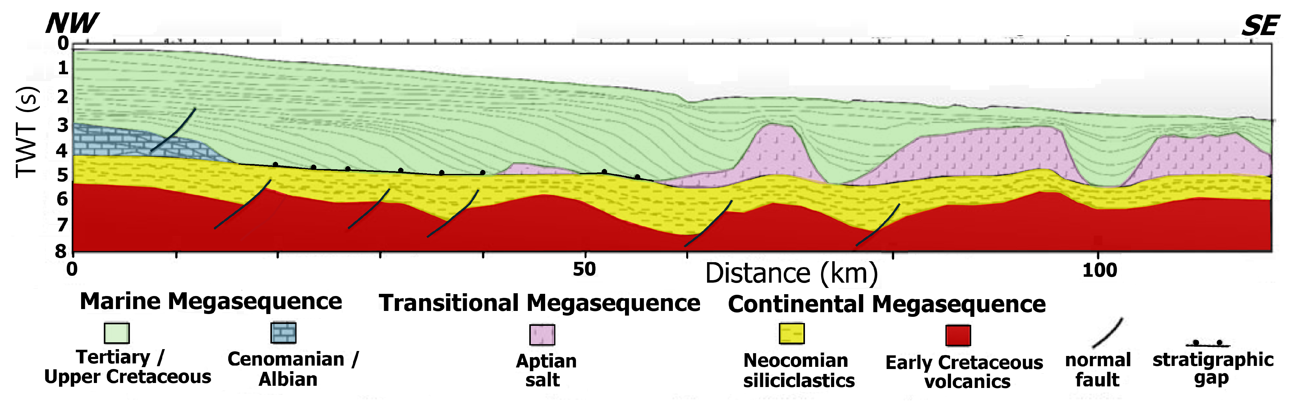
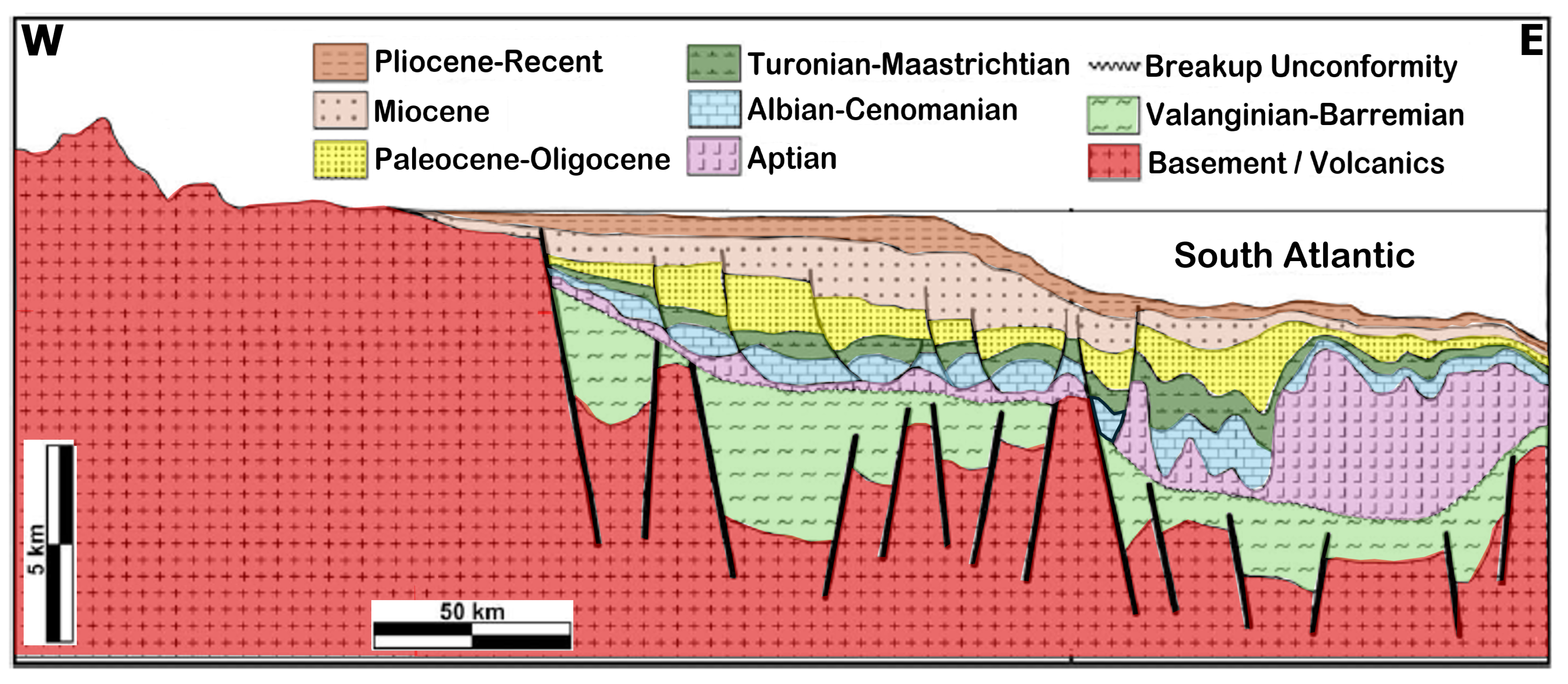
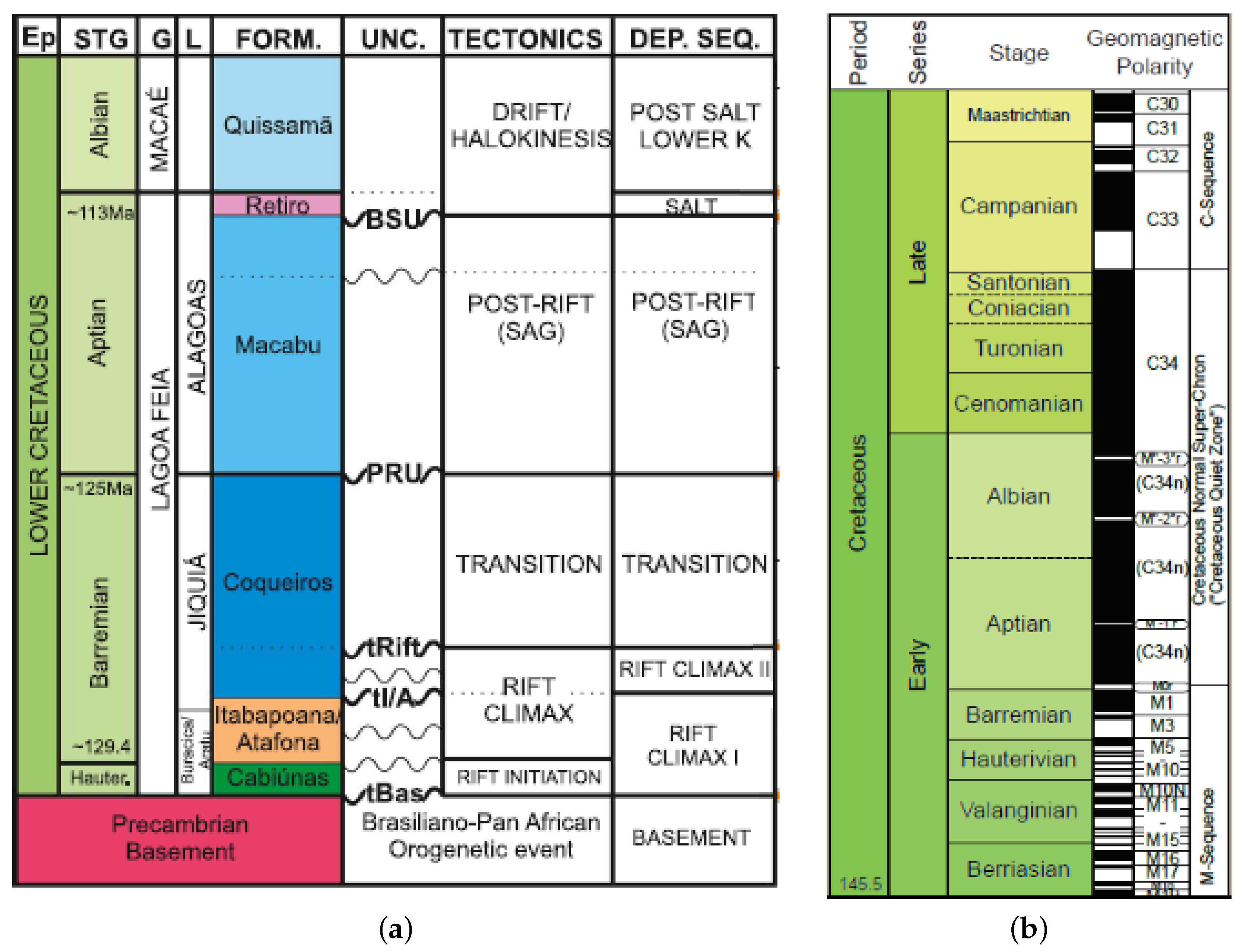
3.1. Campos Basin Geologic Settings

The Campos Basin, located at the South Atlantic continental margin along the southeastern coast of Brazil, is part of the Central Segment of the South Atlantic Ocean. The development of Campos Basin was initiated during the Late-Jurassic/Early-Cretaceous break-up of Gondwana super continent, followed by the opening of the South Atlantic Ocean. Early mechanical subsidence was accomplished by episodic events that reactivated the Proterozoic basement fabric under regional E–W extension. Its stratigraphy includes Early Cretaceous to recent sediments. According to [23], the stratigraphic record of the Campos Basin may be divided into three tectonostratigraphic mega-sequences: Non Marine Rift, Transitional Post-Rift, and Marine Drift, as shown in Figure 5. The Non-Marine Rift is associated with synthetic and antithetic faults forming several half-grabens filled with fluvial-deltaic sediments. The Transitional Post-Rift is characterized by evaporite deposition, where salt movements play important role by controlling stratigraphic and structural features responsible for several exploratory plays. The Marine Drift may be subdivided into a carbonate Restricted Marine sequence (Albian to Turonian) and a siliciclastic Open Marine sequence (Late Cretaceous to Quaternary).

The overall structural style in Campos Basin, exhibited in Figure 6, is controlled by a detachment surface at the base of Aptian salt as proposed by [24]. Above the Aptian detachment the thin-skinned salt tectonics with extensional–proximal and compressional–distal domains have been active during divergent margin phase since the Albian, and is characterized by listric fault-rollover systems, turtle-back structures, raft tectonics, down building diapirs, salt walls, and compressional salt tongues [25,26]. Bellow the detachment, the basement is characterized by a system of horsts and grabens limited by steep normal faults that were active during the rift phase in the Early Cretaceous [27]. As suggested by [24] the basement structure controls the salt tectonic domains, with extensional structures to the West, and diapirs, salt walls, and compressional structures to the East of the main internal basement high.

In a recent paper, [28] has proposed that the Pre-Salt units bellow the detachment are constituted by four depositional sequences that nearly corresponds to the tectonic stages of the rifting: rift initiation, rift climax, transition and post-rift, as shown in Figure 7a. The rift initiation stage is represented by intense tholeiitic volcanic activity. According to [24], the rift climax stage is defined by the development, in the basement, of an extensive NE–SW and NNW–SSE system of horsts and grabens limited by steep normal faults. The rift transition stage is characterized by a carbonate section whose basal portions is associated to the rift climax stage. Carbonate deposits including argillaceous, laminites and spherulitic facies represent the post rift stage as mentioned by [28]. This stage is of great exploratory importance because the entire carbonate section constitutes the main hydrocarbon reservoirs of the Pre-Salt sequence and will be the focus of our magnetic susceptibility and remanence estimates.

3.2. Magnetic Dataset

In Campos Basin, there is a large number of wells where borehole imaging logs and, consequently, magnetic field data from their orientation tools were acquired. Our choice for well 1-RJS-755-RJ is due to the fact that 58 core samples were collected and analyzed in laboratory for magnetic susceptibility along about 550 m of Pre-Salt rocks. The sampled interval includes carbonates on the top of an igneous sequence composed by basalts, diabases, hyaloclastites and breccias. From the total, 47 samples were identified as igneous rocks and 11 as carbonates, all showing high alteration degree [22]. This large number of laboratory measurements provides the necessary control to validate our susceptibility estimates, but since samples were not oriented, the directions of the remanent magnetization were not determined, which makes comparison impossible.

3.2.1. Magnetic Sample Analysis

The laboratory analysis of these samples was performed in the MFK1-FA Multifunction Frequency Kappabridge (AGICO), one of the most sensitive laboratory instruments for measuring both anisotropy of magnetic susceptibility (AMS) and bulk magnetic susceptibility (Figure 8). In addiction to magnetic susceptibility, analysis have also included magnetic hysteresis measurements, IRM (Isothermal Remanent Magnetization) acquisition curves, FORCs (First Order Reversal Curves) and thermomagnetic curves. This set of analysis allows the understanding of the magnetic behavior of these rocks as well as to characterize the main magnetic minerals present in the samples [22].

According to [22], the results of the magnetic susceptibility analysis for the carbonate samples show low values due to the prevailing presence of the diamagnetic minerals (i.e. calcite) in their composition. Measurements for magnetic hysteresis, IRM acquisition, FORCs and thermomagnetic curves for the carbonates have shown extreme noise level due to the low intensity of the magnetic signal. Despite the noise level, the magnetic hysteresis results show curves typical of low coercivity ferromagnetic minerals, while results for both IRM acquisition and thermomagnetic curves were considered as inconclusive. Although weak, the FORC signal of some samples show characteristics of multidomain grains which suggests the presence of detrital magnetite.

For igneous samples, the magnetic susceptibility values were considered lower than would be expected for these kind of rocks. This was interpreted by [22] as consequence of the high alteration degree of the samples. However, the intensity of the magnetic signal was strong enough to allow the magnetic hysteresis and the IRM acquisition to show curves typical of low coercivity ferromagnetic minerals for most of the samples. Two samples, one of basalt and the other of diabase, have shown curves with characteristic behavior of high coercivity ferromagnetic minerals. Analysis of the FORC diagrams have exhibited bi-dimensional data indicating the presence of low coercivity multidomain grains. Thermomagnetic results have indicated that magnetite is the main mineral phase formed but maghemite, greigite, titanomagnetite and possibly pyrite were also identified.

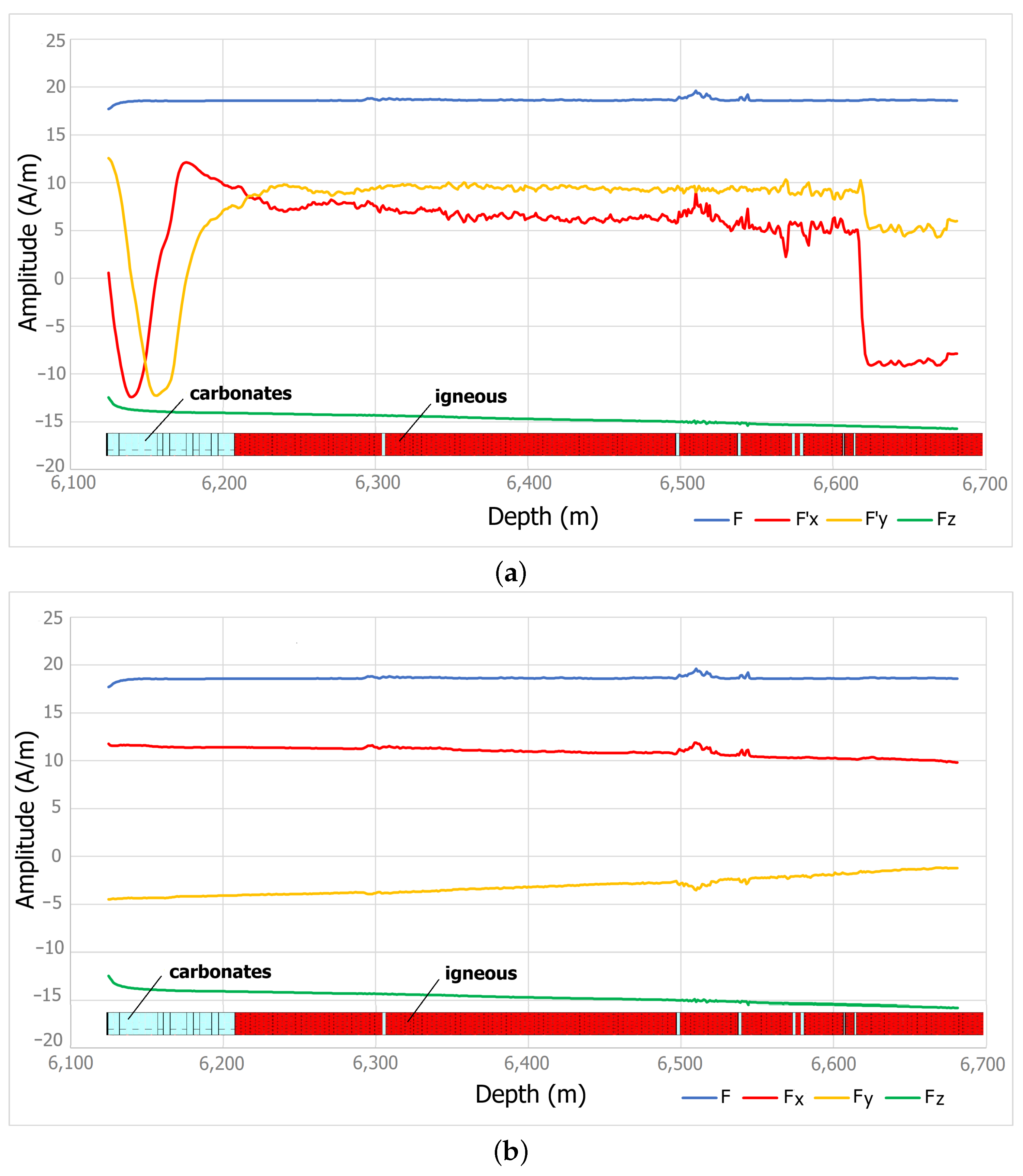
3.2.2. Magnetic Field Data

The magnetic data of well 1-RJS-755-RJ was acquired in Feb/2021 by Schlumberger during a microresistivity imaging survey using a Oil-Base Microimager (OBMI) tool along a depth interval extending from 6125 to 6681 m. The logged segment was composed by a carbonate section extending from 6125 to 6210 m on top of a large basalt section located between 6211 and 6681 m. We have included the lithologic log in Figure 9 and others to allow visual correlation between the measured fields and the corresponding rocks.

The acquired data consists of a set of multiple measurements taken at a 0.15 m interval. However, for the proposed method, only the measurements of depth, magnetic field inclination, magnetic field intensity in x, y and z directions and the PAD1 (see Figure 2b) azimuth angle are strictly necessary. The behavior of the acquired magnetic data, exhibited in Figure 9a, is characterized by fluctuation in the amplitudes of the horizontal components $F_x$ and $F_y$ caused by the tool rotation during acquisition. Components F and $F_z$ are not affected by the tool’s rotation, with F showing an almost constant amplitude as $F_z$ exhibits a slight amplitude decrease with depth.

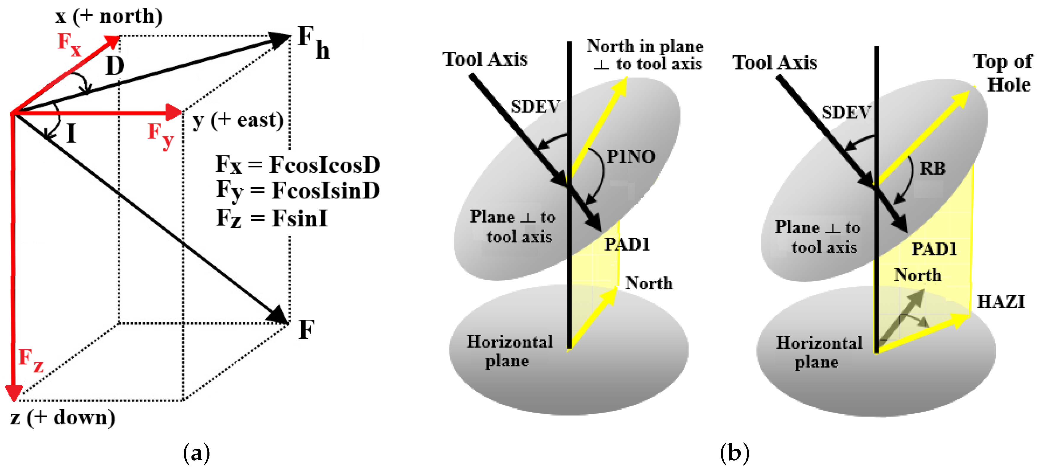
3.3. Magnetic Corrections

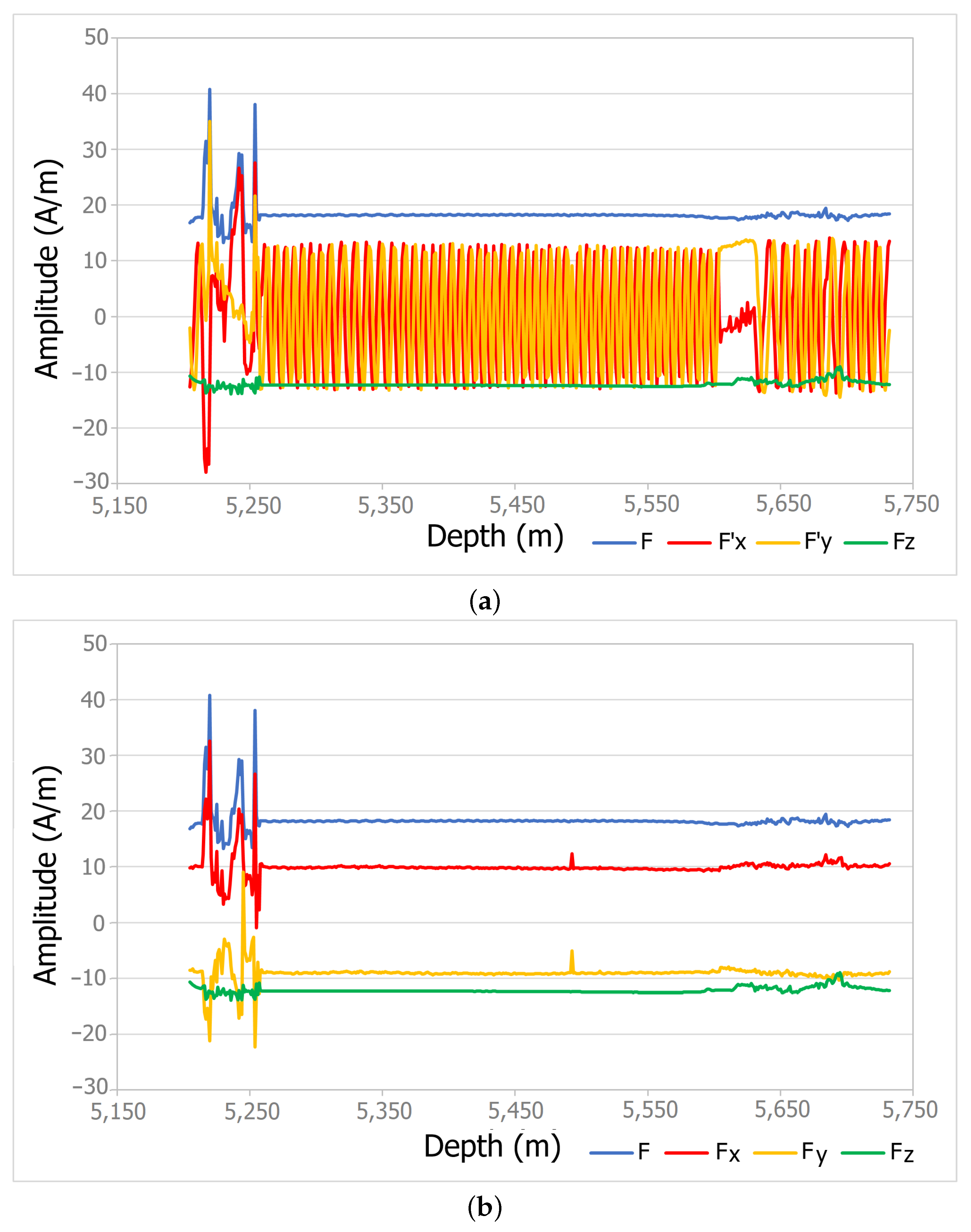
3.3.1. Magnetic Amplitude Correction

The magnetic amplitude correction is the most important correction in this methodology because it recovers the true field amplitudes before doing any estimate. Since the amplitudes of components are the fundamental parameters for all estimates, the precision of this correction directly controls the quality of estimates.

The amplitude fluctuations seen in $F_x$ and $F_y$ components need to be corrected to recover their true values in north and east directions before susceptibility and remanence estimation. Figure 9b exhibits the magnetic field and its components after applying amplitude correction. Besides the expressive reduction in the amplitude fluctuations, there were also significant changes in the magnitudes of the horizontal components after correction. The amplitude of the $F_y$ component was significantly reduced and now it is possible to see a slight increase with depth. On the other hand, $F_x$ component has suffered a small increase in amplitude unveiling a smooth decreases with depth. Total field F and component $F_z$ do not need correction and their form remains unchanged. In terms of behavior, component $F_z$ shows a smooth decrease with depth while the total field F exhibits a flat behavior except by small fluctuations located around depth 6500 m. Even though these localized amplitude variations seem to be directly related to remaining fluctuations in the horizontal components, they also are present in the $F_z$ component, although with a much smaller amplitude that is difficult to see in the scale used in Figure 9 to represent all field components together.

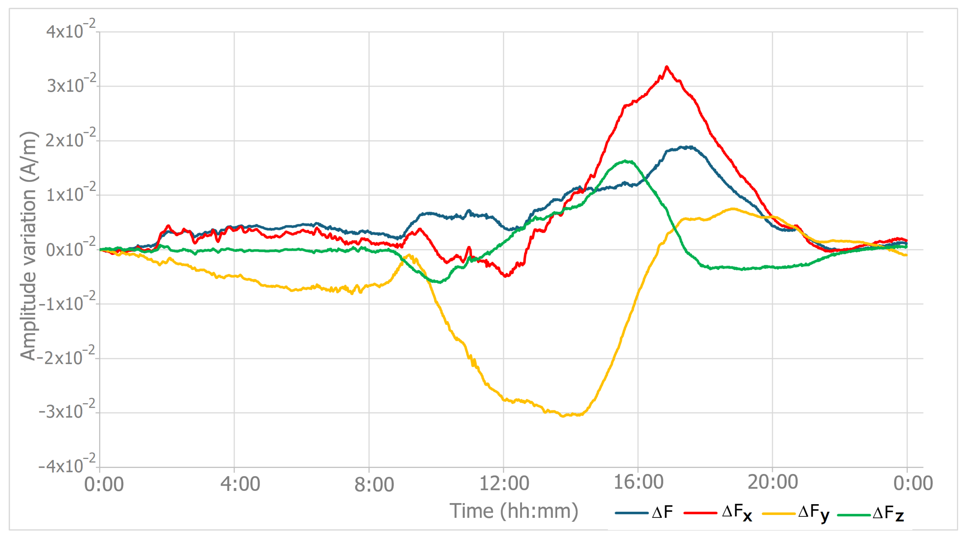
3.3.2. Magnetic Diurnal Variation Correction

It is well known that the Earth’s magnetic field suffers temporal variations during the day caused by interactions between the Sun and electrical charged particles in the ionosphere. Such diurnal variation is characterized by a slow but progressive increase in the field intensity as the solar incidence increases, decreasing towards the background value as the solar incidence reduces. As the logging operations can last for hours, Earth’s magnetic field diurnal variations may occur during such periods of magnetic data acquisition. Once estimates are based mainly on field amplitudes, any temporal variation in the field introduces localized errors in the estimates. If the logging time interval is known, it is possible to remove such variations using for that the magnetic field behavior registered by the closest magnetic observatory. In the case of well 1-RJS-755-RJ, the magnetic field variations during logging operation (from 02:26 to 07:58 AM) was corrected using records obtained by Vassouras Magnetic Observatory (VSS) in Rio de Janeiro, Brazil, the closest to the well location. Figure 10 shows the variations of the Earth’s magnetic field and its components along the day of logging (10 February 2021). Because the amplitude of field variations were not large during operation period, corrections were small and visually imperceptible in the scale used to represent the field and its components together and will not be shown here.

After all corrections the measured magnetic field and its components can be used in the magnetic susceptibility and remanence estimates. Due to the visualization difficulties caused by the large scale necessary to show all components together, we exhibit in Figure 11 only the F field, which allows better evaluation of rock’s magnetic response in depth. Notice that the field response to the igneous rocks becomes more evident only below the base of the first interval (around 6300 m). It is important to notice that there is no significant change in the transition between the carbonates and the first igneous interval, who shows only a slight increase in field amplitude with depth. Since the first interval represents the top of the igneous sequence, it seems possible that it has been exposed to a higher alteration degree, which may have reduced its contribution to the measured magnetic field.

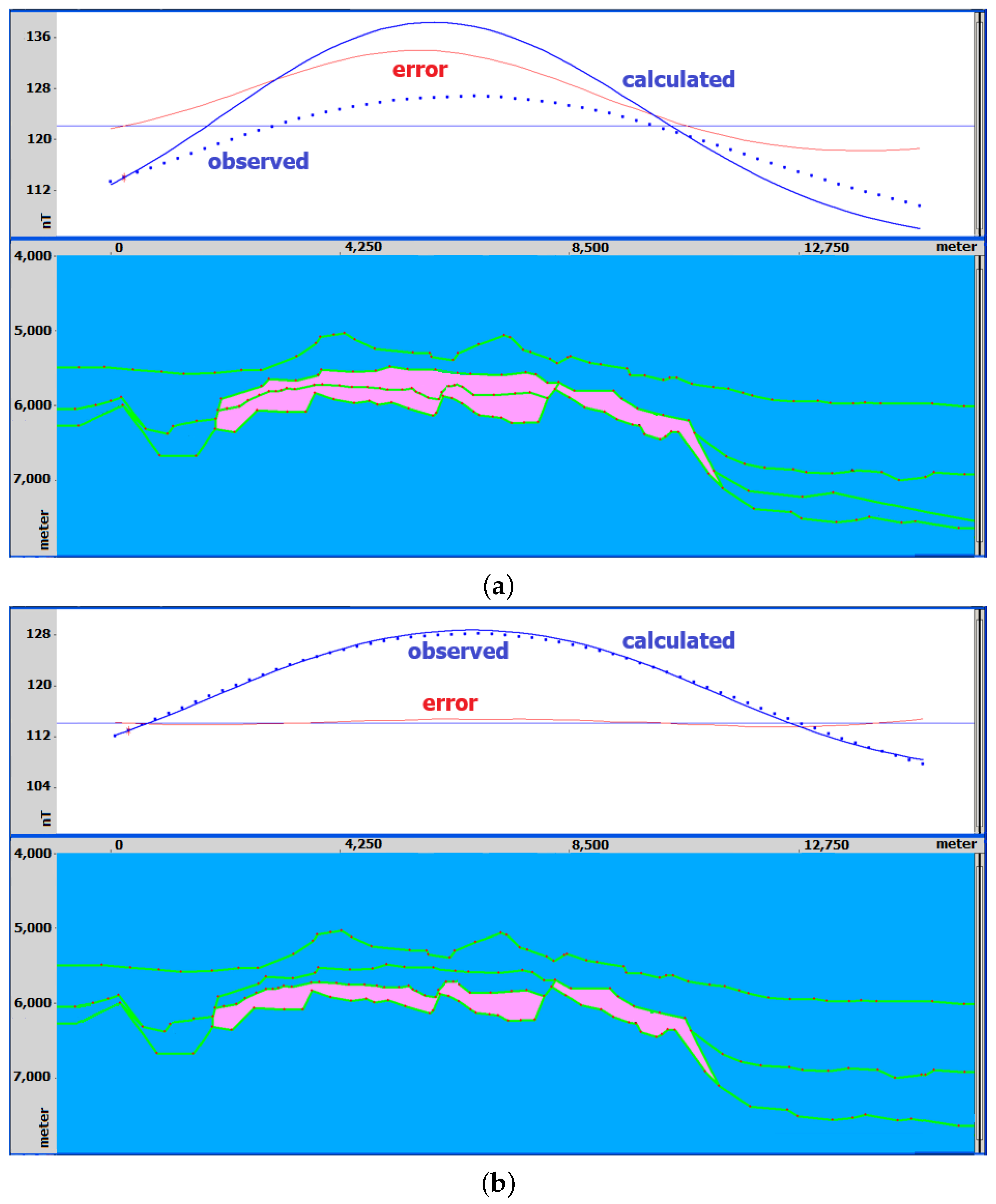
3.4. Magnetic Susceptibility Estimates

According to Equation (4), estimates of magnetic susceptibility and remanence require knowing the behavior of the Earth’s magnetic field H in depth at the location of well 1-RJS-755-RJ on the date of logging (10 February 2021). One way of doing this is considering the IGRF (International Geomagnetic Reference Field) as a good representation of field H. However, the IGRF only represents the dipolar portion of the Earth’s field and does not take into account any regional field. Another option is the Enhanced Magnetic Model 2017 (EMM2017), a mathematical model also considered to satisfactorily represent the Earth’s magnetic field. The EMM2017 is a compilation of satellite, aerial, marine and terrestrial data, which uses spherical harmonics of the scalar magnetic potential of degree and order 790 to represent the field [30]. As it includes regional data into its model, it seems to be a better choice to represent H, assuming the differences to the measured field F are just the local field changes in depth caused by the presence of igneous rocks. Although this is a strong assumption, the fact that the magnetic field decays rapidly with distance allows us to assume that the contribution to the magnetic field caused by rocks close to the sensor will by far overcome those of deeper portions of the basin. Therefore, we chose to use the EMM2017 to represent the Earth’s magnetic field H in our estimates. Figure 12a shows the variation in depth of the Earth’s magnetic field according to the EMM2017 model. The small amplitude variations in depth of Earth’s field model are not visible in the scale of Figure 12a and the curves looks almost constant. Moreover, visual comparison with the field amplitudes measured in well 1-RJS-755-RJ after correction (Figure 9b) confirms EMM2017 model as a good approximation to Earth’s magnetic field. The difference between measured (F) and model field (H) is shown in Figure 12b. The small differences in amplitude result from the local geologic variations as can be seen by the correlation with the lithologic log.

Estimates of magnetic susceptibility $\chi$ for the carbonate interval (6125 to 6210 m) is simpler because carbonates are assumed do not acquire remanent magnetization and can be achieved applying Equation (3). The statistics for magnetic susceptibility estimates for the carbonate interval in the different directions is shown in

Table 1. Statistics for magnetic susceptibility estimates in different directions for the carbonate interval (6125 to 6210 m) of well 1-RJS-755-RJ. The $\chi$ value represents the mean susceptibility according to Equation (7).

	$\mathit{\chi }$	${\mathit{\chi }}_{\mathit{x}}$	${\mathit{\chi }}_{\mathit{y}}$	${\mathit{\chi }}_{\mathit{z}}$
Minimum	$-5.6\times {10}^{-2}$	$-5.9\times {10}^{-2}$	$-2.6\times {10}^{-1}$	$-5.8\times {10}^{-2}$
Maximum	$-1.0\times {10}^{-2}$	$-2.9\times {10}^{-2}$	$-1.8\times {10}^{-1}$	$6.4\times {10}^{-2}$
Mean	$-1.4\times {10}^{-2}$	$-5.2\times {10}^{-2}$	$-2.3\times {10}^{-1}$	$4.8\times {10}^{-2}$
Standard deviation	$8.7\times {10}^{-3}$	$8.0\times {10}^{-3}$	$2.2\times {10}^{-2}$	$2.3\times {10}^{-2}$

. Analysis of the statistics shows results dominated by negative values, which means that the measured field is smaller than the predicted by the Earth’s model field. Since carbonates are mainly constituted by calcite, a diamagnetic mineral, i.e., a mineral whose magnetic response is in the opposite direction to the applied field, this result seems reasonable. In terms of absolute amplitude, estimated susceptibility are, at least, one order of magnitude higher than the average values proposed for carbonates in the literature (Figure 13) as shown by [31]. However, we must consider that literature values are world averages. It should include several types of carbonates in different stratigraphic positions. On the other hand, our carbonates are located directly on the top of igneous rocks whose strong magnetic field may be influencing the measurements taken on the carbonates right above and inducing higher susceptibility values.

The interval extending from 6211 to 6681 m is composed by igneous rocks. The lithologic profile included in Figure 9 shows that the igneous interval can be divided into six smaller segments separated by tiny carbonate layers. These intervals extend from 6211 to 6300 m, 6305 to 6495 m, 6500 to 6535 m, 6540 to 6570 m, 6585 to 6605 m and 6620 to 6681 m. Because both susceptibility and remanence can be different in these igneous intervals, estimates were be done separately using Equation (7) after solving the system proposed in Equation (5) for each interval. The estimates for the six igneous intervals are exhibited in

Table 2. Magnetic susceptibility ($\chi$) and remanence ($M_R$) estimates for the six igneous intervals of well 1-RJS-755-RJ.

	Interval (m)
Estimates	6211–6300	6305–6495	6500–6535	6540–6570	6585–6605	6620–6681
${\chi }_x$	$2.3\times {10}^{-1}$	$8.7\times {10}^{-1}$	$5.5\times {10}^{-1}$	$8.6\times {10}^{-1}$	$5.6\times {10}^{-1}$	$7.2\times {10}^{-1}$
${\chi }_y$	$-8.2\times {10}^{-1}$	$-9.3\times {10}^{-1}$	$-7.0\times {10}^{-1}$	$-5.9\times {10}^{-1}$	$-5.0\times {10}^{-1}$	$-9.3\times {10}^{-1}$
${\chi }_z$	$1.0\times {10}^0$	$9.9\times {10}^{-1}$	$3.8\times {10}^{-1}$	$5.0\times {10}^{-1}$	$9.2\times {10}^{-1}$	$1.0\times {10}^0$
$\chi$	$1.4\times {10}^{-1}$	$3.1\times {10}^{-1}$	$7.8\times {10}^{-2}$	$2.6\times {10}^{-1}$	$3.3\times {10}^{-1}$	$2.6\times {10}^{-1}$
$M_{R_x}$ (A/m)	$-7.9\times {10}^{-1}$	$-1.4\times {10}^0$	$-1.2\times {10}^0$	$-1.8\times {10}^0$	$-1.9\times {10}^0$	$-2.1\times {10}^0$
$M_{R_y}$ (A/m)	$1.7\times {10}^0$	$2.8\times {10}^0$	$3.1\times {10}^0$	$3.4\times {10}^0$	$3.7\times {10}^0$	$4.3\times {10}^0$
$M_{R_z}$ (A/m)	$-1.1\times {10}^0$	$-1.7\times {10}^0$	$-1.9\times {10}^0$	$-2.1\times {10}^0$	$-2.1\times {10}^0$	$-2.5\times {10}^0$
$M_R$ (A/m)	$2.2\times {10}^0$	$3.6\times {10}^0$	$3.8\times {10}^0$	$4.4\times {10}^0$	$4.7\times {10}^0$	$5.4\times {10}^0$

. Since Equation (5) assumes both susceptibility and remanence as constant along these intervals the estimates for each component are represented by single values.

The results presented in Table 2 show magnitude values of susceptibility around $1\times {10}^{-1}$ SI unit, which is within the expected range for igneous rocks according to [31] (Figure 13). In terms of remanence, the estimated values ranging from around $2.0$ to over 6.0 ${\mathrm{Am}}^{-1}$ are lower in amplitude when compared to the strength of actual Earth’s magnetic field, whose lower values are around 16 ${\mathrm{Am}}^{-1}$. Low values of the Earth’s magnetic field may be related to geomagnetic field reversals, as proposed by [32]. In a paper describing numerical simulations of geomagnetic field reversals, Ref. [32] has found that just before each reversal the intensity of the magnetic field became very weak. So, it seems possible that when those igneous rocks acquired magnetization, the Earth’s field was in a reversal process. To reinforce this hypothesis, the geomagnetic polarity scale shown in Figure 7b indicates that the Hauterivian, the time stage when these rocks were formed, was undergoing intense polarity changes. Another possibility is that the intensity of the remanent field was not fully preserved inside these rocks along the time. In addiction, the fact that both $\chi$ and $M_R$ estimates do not show widely disperse values gives confidence to the results.

Equations (8)–(10) allow estimates of both inclination $I_R$ and declination $D_R$ of the remanent magnetic field at the time those igneous rocks were formed. The results for the six igneous intervals of well 1-RJS-755-RJ are very consistent as shown in

Table 3. Inclination $I_R$ and declination $D_R$ estimates for remanence of the six igneous intervals in well 1-RJS-755-RJ.

Interval (m)	${\mathit{I}}_{\mathit{R}}{(}^{\circ })$	${\mathit{D}}_{\mathit{R}}{(}^{\circ })$
6211–6300	$-29.98$	$114.63$
6305–6495	$-29.14$	$115.96$
6500–6535	$-29.43$	$112.05$
6540–6570	$-28.20$	$117.68$
6585–6605	$-27.53$	$116.66$
6620–6681	$-26.96$	$116.32$

, which gives credibility to the estimates. In terms of remanence inclination the results point to an inclination angle between $-{27}^{\circ }$ and $-{30}^{\circ }$ pointing to the same direction of the actual Earth’s field but with a smaller angle since the actual field inclination at well position is about $-{45}^{\circ }$. The declination estimates show small values dispersion ranging from around ${112}^{\circ }$ to ${118}^{\circ }$, values that are very different from today’s field at well location, which is around ${24}^{\circ }$. However, the geomagnetic field reversal simulations of [32] indicates that during a reversal the field not only becomes weaker, but also multiple poles may appear in different parts of the globe. The low field intensity associated to the unusual declination angle may support the hypothesis that the igneous rocks may have acquired magnetization during a period of intense magnetic field changes, as illustrated by the geomagnetic polarity scale of Figure 7b (Hauterivian stage). As no remanent inclination and declination measures are available to compare, it is difficult to extend this discussion since, in the worst hypothesis, we may be speculating upon not valid results.

As mentioned in Section 3.2, magnetic susceptibility laboratory measurements were made in 58 rock samples distributed along the analyzed interval. The laboratory values are plotted together with the susceptibility estimates in Figure 14. For the carbonate interval estimate, results show values one order of magnitude higher than those measured in the lab. It is possible that the close presence of igneous rocks may be influencing the measured field and, consequently, the susceptibility estimates. Estimates for the igneous rocks presented better results when compared with the lab analysis. The first igneous interval, for instance, shows estimates that are very close to the measurements. For second and third interval estimates are a little lower than the measures while the predictions for the remaining intervals show higher values than the measurements. Taken into account that the process uses only the magnetic field acquired inside the well for its estimates, we consider these results as satisfactory to provide susceptibility and remanence values for forward magnetic modeling purposes.

4. Conclusions

Results achieved with this research lead to the conclusion that both magnetic susceptibility and remanent magnetic field can be satisfactorily estimated for forward magnetic modeling purposes from the magnetic field acquired by orientation tools in borehole imaging logs. The methodology can also be applied in mining boreholes if they have acquired the magnetic field. The use for magnetostratigraphy, however, depends on a resolution improvement in the acquired magnetic data.

When applied to real data the proposed methodology has estimated magnetic susceptibility values inside the range of values published in the literature for igneous rocks, and very close to laboratory measurements taken from rock samples collected in the well. The methodology can be improved by doing adjustments in the correction of the rotation tool effect, the most important correction. The choice of the Earth’s magnetic field model can also be improved by taking always the most complete model. Finally, the use of a base magnetometer near the well may provide better data to the correction of diurnal field variation.

Although measurements of intensity, inclination and declination for magnetic remanence were not available to validate our estimates, the small values dispersion of each variable and the consistence of the results in terms of what we would expect for a magnetic field, gives confidence to the process. The promising results achieved here has proved that the proposed methodology is able to provide reliable susceptibility values for magnetic forward modeling and inversion, specially in the case of hydrocarbon exploration where direct measures are rare. Applications in mining and magnetostratigraphy may also be possible but require further investigations.

References

1. Laier, A.P.; Jesus, C.M.; Ferraz, E.K.P.; Caires, A.C.B.; Júnior, J.C. Implicações Exploratórias da Orientação de Perfis de Imagem. In Proceedings of the XI Seminário de Interpretação Exploratória, Petrobras, Rio de Janeiro, Brazil, 12 March 2018. [Google Scholar]
2. Oliveira, J.A.B. Modelagens Magnéticas Como Suporte ao Mapeamento de Rochas Ígneas; Nota técnica; Petrobras: Rio de Janeiro, Brazil, 2017. [Google Scholar]
3. Pozzi, J.P.; Martin, J.P.; Pocachard, J.; Feinberg, H.; Galdeano, A. In-situ magnetostratigraphy: Interpretation of magnetic logging in sediments. Earth Planet. Sci. Lett. 1988, 88, 357–373. [Google Scholar] [CrossRef]
4. Nelson, P.H. Magnetic susceptibility logs from sedimentary and volcanic environments. In Proceedings of the SPWLA 34th Annual Logging Symposium, Calgary, AB, Canada, 13–16 June 1993. [Google Scholar]
5. Broding, R.; Zimmerman, C.; Somers, E.; Wilhelm, E.; Stripling, A. Magnetic well logging. Geophysics 1952, 17, 1–26. [Google Scholar] [CrossRef]
6. Lalanne, B.; Bouisset, P.; Pages, G.; Pocachard, J. Magnetic Logging: Borehole Magnetostratigraphy and Absolute Datation in Sedimentary Rocks. In Proceedings of the Middle East Oil Show, Manama, Bahrain, 16–19 November 1991; SPE-21437-MS. pp. 841–850. [Google Scholar]
7. Pages, G.; Boutemy, Y.; Barthies, V.; Pocachard, J. Wireline Magnetostratigraphy Principles And Field Results. In Proceedings of the SPWLA 35th Annual Logging Symposium, Tulsa, OK, USA, 19–22 June 1994. [Google Scholar]
8. Emilia, D.A.; Allen, J.W.; Chessmore, R.B.; Wilson, R.B. The DOE/Simplec magnetic susceptibility logging system. In Proceedings of the SPWLA 22nd Annual Logging Symposium, Mexico City, Mexico, 23–26 June 1981. [Google Scholar]
9. Scott, J.H.; Seeley, R.L.; Barth, J.J. A magnetic susceptibility well-logging system for mineral exploration. In Proceedings of the SPWLA 22nd Annual Logging Symposium, Mexico City, Mexico, 23–26 June 1981. [Google Scholar]
10. McNeill, J.D.; Hunter, J.A.; Bosnar, M. Application of a borehole induction magnetic susceptibility logger to shallow lithological mapping. J. Environ. Eng. Geophys. 1996, 1, 77–90. [Google Scholar] [CrossRef]
11. Leslie, K.; Foss, C.A.; Hillan, D.; Blay, K. A downhole magnetic tensor gradiometer for developing robust magnetisation models from magnetic anomalies. In Proceedings of the Iron Ore, Perth, WA, Australia, 13–15 July 2015; pp. 1–11. [Google Scholar]
12. Barber, T.; Anderson, B.; Mowat, G. Using induction tools to identify magnetic formations and to determine relative magnetic susceptibility and dielectric constant. Log Anal. 1995, 36, 16–26. [Google Scholar]
13. Mitchell, J. Monitoring Lithology Variations in Drilled Rock Formations Using NMR Apparent Magnetic Susceptibility Contrast. Appl. Magn. Reson. 2020, 51, 205–219. [Google Scholar] [CrossRef]
14. Huret, E.; Thiesson, J.; Tabbagh, A.; Galbrun, B.; Collin, P. Improvement of cyclostratigraphic studies by processing of high-resolution magnetic susceptibility logging: Example of PEP1002 borehole (Bure, Meuse, France). Comptes Rendus Geosci. 2011, 343, 379–386. [Google Scholar] [CrossRef]
15. Crow, H.L.; Hunter, J.A.; Olson, L.C.; Pugin, A.J.M.; Russell, H.A.J. Borehole geophysical log signatures and stratigraphic assessment in a glacial basin, southern Ontario. Can. J. Earth Sci. 2018, 55, 829–845. [Google Scholar] [CrossRef]
16. Nowaczyk, N.R. Logging of Magnetic Susceptibility. In Tracking Environmental Change Using Lake Sediments: Basin Analysis, Coring, and Chronological Techniques; Last, W.M., Smol, J.P., Eds.; Springer: Dordrecht, The Netherlands, 2001; pp. 155–170. [Google Scholar] [CrossRef]
17. Bloemendal, J.; Tauxe, L.; Valet, J.P. High-resolution, whole-core magnetic susceptibility logs from LEG 1081. In Ocean Drilling Program: Initial Report; Ocean Drilling Program; Texas A&M University: College Station, TX, USA, 1986; Volume 108, p. 1005. [Google Scholar]
18. Dalan, R.A. A review of the role of magnetic susceptibility in archaeogeophysical studies in the USA: Recent developments and prospects. Archaeol. Prospect. 2008, 15, 1–31. [Google Scholar] [CrossRef]
19. To, T.H.; Nguyen, T.V.; Nguyen, L.K.; Dinh, H.D. A review of the applications of magnetic susceptibility measurements for improved reservoir characterization. J. Min. Earth Sci. 2022, 63, 25–34. [Google Scholar] [CrossRef] [PubMed]
20. Cheung, P.; Hayman, A.; Vessereau, P.; Verges, P.; Laval, L.; Yerbes, M.; Rylander, E. In Situ Correction of Wireline Triaxial Accelerometer and Magnetometer Measurements. In Proceedings of the SPWLA 48th Annual Logging Symposium, Austin, TX, USA, 3–6 June 2007. [Google Scholar]
21. ANP—Agência Nacional de Petróleo, Gás Natural e Biocombustíveis. Boletim da Produção de Petróleo e Gás Natural—06/2024. 2024. Available online: https://www.gov.br/anp/pt-br/centrais-de-conteudo/publicacoes/boletins-anp/boletins/arquivos-bmppgn/2024/junho.pdf (accessed on 6 August 2024).
22. Rodrigues, A.N.G. Propriedades Magnéticas do poço 1-RJS-755-RJ (Urissanê), Intervalo 6137.70–6683.00 m, Bacia de Campos (Brasil); Relatório Interno; Petrobras: Rio de Janeiro, Brazil, 2021. [Google Scholar]
23. Cainelli, C.; Mohriak, W.U. Some remarks on the evolution of sedimentary basins along the Eastern Brazilian continental margin. Episodes J. Int. Geosci. 1999, 22, 206–216. [Google Scholar] [CrossRef] [PubMed]
24. Fetter, M. The role of basement tectonic reactivation on the structural evolution of Campos Basin, offshore Brazil: Evidence from 3D seismic analysis and section restoration. Mar. Pet. Geol. 2009, 26, 873–886. [Google Scholar] [CrossRef]
25. Cobbold, P.R.; Szatmari, P. Radial gravitational gliding on passive margins. Tectonophysics 1991, 188, 249–289. [Google Scholar] [CrossRef]
26. Demercian, S.; Szatmari, P.; Cobbold, P.R. Style and pattern of salt diapirs due to thin-skinned gravitational gliding, Campos and Santos basins, offshore Brazil. Tectonophysics 1993, 228, 393–433. [Google Scholar] [CrossRef]
27. Chang, H.K.; Kowsmann, R.O.; Figueiredo, A.M.F.; Bender, A.A. Tectonics and stratigraphy of the East Brazil Rift system: An overview. Tectonophysics 1992, 213, 97–138. [Google Scholar] [CrossRef]
28. Strugale, M.; Schmitt, R.S.; Cartwright, J. Basement geology and its controls on the nucleation and growth of rift faults in the northern Campos Basin, offshore Brazil. Basin Res. 2021, 33, 1906–1933. [Google Scholar] [CrossRef]
29. Ogg, J.G.; Ogg, G.M.; Gradstein, F.M. The Concise Geologic Time Scale; Cambridge University Press: Cambridge, UK, 2008. [Google Scholar]
30. NOAA/NCEI—National Center for Environmental Information. Enhanced Magnetic Model (EMM). 2022. Available online: https://www.ngdc.noaa.gov/geomag/EMM (accessed on 6 August 2024).
31. Lowrie, W. Fundamentals of Geophysics; Cambridge University Press: Cambridge, UK, 1997. [Google Scholar]
32. Glatzmaiers, G.A.; Roberts, P.H. A three-dimensional self-consistent computer simulation of a geomagnetic field reversal. Nature 1995, 377, 203–209. [Google Scholar] [CrossRef]
Figure 1. Forward modeling example of Brazilian Pre-Salt exploration. The upper panels show the magnetic profiles. The models are shown in the lower panels where the blue regions are the non-magnetic rocks while the pink regions represent the igneous rocks. The green lines are the interface between layers as interpreted from seismic data. (a) The initial model with a thicker igneous package. (b) The final model suggesting less igneous rocks, which was confirmed by drilling (modified from [2]).
Applsci 15 02873 g001
Figure 2. Graphic illustration of some important definitions. (a) Spatial relationship between the components, F x , F y and F z , of the magnetic field described in terms of three parameters: magnitude F, inclination I and declination D. The sign convention for field and its components is: x positive to north, y positive to east and z positive downward. (b) Representation of the meaning of four tool angles, SDEV, HAZI, RB and P1NO, which describes tool’s orientation in the geographical coordinate system (modified from [20]).
Applsci 15 02873 g002
Figure 3. Example of the amplitude fluctuation caused by tool’s rotation in a typical well. The strong amplitude fluctuations occurring in the horizontal components shown in (a) were greatly reduced after correction, as exhibit in (b).
Applsci 15 02873 g003
Figure 4. Geographic location of well 1-RJS-755-RJ at 2950 m water depth in the Campos Basin, Brazil. Contour lines represent the bathymetry (modified from [22]).
Applsci 15 02873 g004
Figure 5. Schematic dip-oriented geological section in the Campos showing the tectonostratigraphic mega-sequences (modified from [23]).
Applsci 15 02873 g005
Figure 6. Structural section through central Campos Basin showing the dominant detached structural style (modified from [24]).
Applsci 15 02873 g006
Figure 7. Simplified stratigraphic and tectonic framework of Campos Basin. (a) The main unconformities are: BSU (Base-Salt Unconformity), PRU (Post-Rift Unconformity), tRift (top Rift), tI/A (top Itabapoana/Atafona fms.), tBas (top basement), modified from [28]. (b) Geomagnetic polarity time scale for Cretaceous, modified from Concise Geologic Time Scale [29].
Applsci 15 02873 g007
Figure 8. The MFK1-FA instrument used to measure the magnetic susceptibility in 58 core samples collected in well 1-RJS-755-RJ (https://www.agico.cz/text/products/olddev/olddev.php, (accessed on 31 January 2025)).
Applsci 15 02873 g008
Figure 9. Magnetic field and its components as acquired in well 1-RJS-755-RJ before (a) and after amplitude correction (b). Notice the significant change in the magnitude of the horizontal components after correction of the disturbance caused by tool rotation. The lithologic log is included for illustration.
Applsci 15 02873 g009
Figure 10. Diurnal variation of Earth’s magnetic field and its components on 10 February 2021 according to Vassouras Magnetic Observatory (VSS) in Rio de Janeiro, Brazil. The logging operation was from 02:26 to 7:58 AM, a period of relatively small variations.
Applsci 15 02873 g010
Figure 11. Measured magnetic field F after corrections. The field components were omitted to allow better visualization of the variation caused by the presence of igneous rocks. The lithologic log is included for illustration.
Applsci 15 02873 g011
Figure 12. (a) The Earth’s magnetic field in depth at position of well 1-RJS-755-RJ according to the EMM2017 model. (b) Differences in depth between the field measured in well 1-RJS-755-RJ and Earth’s magnetic field model. These small differences in amplitude are caused by the local geologic variation in depth. The lithologic log is included for illustration.
Applsci 15 02873 g012
Figure 13. Ranges and mean values of the magnetic susceptibility of the most common rock types (modified from [31]). For comparison, susceptibility estimates from our methodology are plotted as yellow circles (igneous rocks) and red circle (carbonates).
Applsci 15 02873 g013
Figure 14. Magnetic susceptibility estimates for well 1-RJS-755-RJ and the result of 58 susceptibility laboratory measurements made in rock samples. The lithologic log along the well is exhibited in the base of the chart for illustration.
Applsci 15 02873 g014