Inversion of Elastic and Fracture Parameters in Tilted Transverse Isotropic Media with Parameter Standardization

Abstract

This study addresses inversion challenges in tilted transverse isotropic (TTI) media affected by inclined fractures. A new method is proposed to derive the reflection coefficient for such media, combining scattering theory with the steady-phase method. To enhance inversion accuracy and stability, a scale normalization technique is introduced. The approach improves parameter consistency during the inversion process. The results highlight the potential of this method to offer valuable technical support for fractured reservoir exploration and development.

1. Introduction

In the exploration and development of tight carbonate reservoirs, fracture development plays a crucial role in determining reservoir permeability and the formation of reservoir space. The presence of fractures induces anisotropy in the subsurface medium, which manifests as variations in elastic properties depending on the direction. To quantitatively characterize this anisotropy, specific anisotropy parameters for different types of media are proposed (Thomsen, 1986; Rüger, 1996; Tsvankin, 1997) [1,2,3]. The petrophysical characterization of fractured media is a critical aspect of understanding the behavior of reservoirs, particularly in terms of permeability and anisotropy. Several models have been proposed to represent the effects of fractures on the elastic properties of subsurface materials. These include Hudson’s micro-fracture model (Hudson, 1980, 1981) [4,5], Schoenberg’s linear slip model (Schoenberg, 1980) [6], and the moving mesh method (Ivančić and Solovchuk, 2022) [7]. Among the most widely used are Hudson’s micro-fracture model and Schoenberg’s linear slip model, both of which provide essential frameworks for representing fractured rock as equivalent anisotropic media. Schoenberg further introduced the concepts of normal weakness ${\delta }_N$ and tangential weakness ${\delta }_T$ to quantitatively assess the anisotropy induced by fractures, offering a means to characterize fracture-related anisotropy in terms of material behavior. Building upon this, Bakulin (2000) developed a relationship between the fracture weakness parameter [8], the Thomsen anisotropy parameters, and fracture density, providing a unified theoretical foundation for describing the anisotropic effects of fractures in a comprehensive manner. These advancements have significantly improved our ability to model and interpret the complex anisotropic behavior of fractured reservoirs, offering valuable insights into reservoir exploration and development (Figure 1) [9].

The azimuthal AVO (Amplitude Versus Offset) inversion has emerged as a powerful and reliable technique for predicting fracture parameters, playing a pivotal role in characterizing subsurface anisotropy and heterogeneity (Bachrach, 2015; Li, 2022; Chen, 2024) [10,11,12]. Central to the success of azimuthal AVO inversion is the accurate estimation of reflection coefficients, which are highly sensitive to fracture characteristics, such as orientation and density. The response of fractured media is strongly dependent on the orientation of the fractures relative to the seismic wave propagation direction. When fractures are vertically oriented, the medium can be effectively modeled as a horizontally layered transversely isotropic (HTI) medium. Numerous studies have focused on deriving and refining reflection coefficient models for HTI media to better understand the seismic response of such systems (Rüger, 1997; Chen et al., 2017) [13,14]. In contrast, when fractures are horizontally oriented, the medium can be treated as a vertically layered transversely isotropic (VTI) medium, and extensive research has been conducted on the reflection coefficients for VTI media, providing insights into the seismic behavior of such systems (Shaw and Sen, 2004; Zhang et al., 2019) [15,16]. When fractures are inclined, the resulting anisotropy becomes more intricate, and the medium is typically described using the tilted transversely isotropic (TTI) model. This model captures the more complex interactions between fracture geometry and seismic waves, and recent advancements have enhanced the understanding of fracture tilt effects on the elastic properties of the medium (Pan et al., 2021; Zhao et al., 2024) [17,18].

In this study, we derive the reflection coefficients for TTI media, considering the influence of a set of inclined fractures with rotational invariance. Our approach is grounded in the assumption of weak anisotropy and the theory of seismic scattering. In the context of seismic inversion, a major challenge lies in addressing the inconsistent scales of inversion parameters, which can lead to inaccuracies in the inversion process. To overcome this issue, we propose a novel inversion equation that transforms the parameters into a uniform scale, thereby improving the reliability of the inversion results. To demonstrate the effectiveness of our method, we perform validations using both synthetic model data and actual field data. The results underscore the practical applicability of our approach to enhance seismic inversion accuracy in anisotropic media.

2. Theory and Method

2.1. Derivation of the Reflection Coefficient Equation

In the investigation of the stiffness matrix for anisotropic media, we consider a specific case involving a group of horizontal, rotationally invariant fractures within a vertically transversely isotropic (VTI) medium. The stiffness matrix for this configuration is derived and expressed as follows:

$$C^{VTI}=C^{Iso}+C_f^H$$

(1)

where $C^{Iso}$ represents the stiffness coefficient matrix of the background isotropic medium while $C_f^H$ corresponds to the stiffness coefficient matrix induced by a single group of horizontal fractures. Similarly, the stiffness coefficient matrix of HTI media, which is caused by a set of vertical, rotationally invariant fractures, can be expressed as the sum of the background isotropic medium’s stiffness matrix and the matrix resulting from the vertical fractures. Building on this principle of superposition, the stiffness matrix for TTI media can be formulated as the sum of the stiffness matrix for the background isotropic medium and the stiffness matrix induced by a set of inclined fractures. Furthermore, the stiffness matrix resulting from a single group of inclined fractures in TTI media can be decomposed into two components: one from the vertical fractures and the other from the horizontal fractures. Therefore, the total stiffness coefficient matrix for the TTI medium is given by the following:

$$C^{TTI}=C^{Iso}+C_f^T=C^{Iso}+C_{f^{\prime }}^V\cos \xi +C_{f^{\prime }}^H\sin \xi$$

(2)

where $\xi$ represents the angle between the fracture and the vertical direction in the TTI medium. $C_{f^{\prime }}^V\cos \xi$ refers to the difference in the stiffness matrix caused by the inclined fracture in the vertical direction, and the influence of this component on the seismic amplitude is solely dependent on the incident angle. On the other hand, $C_{f^{\prime }}^H\sin \xi$ represents the difference in the stiffness matrix due to the inclined fracture in the horizontal direction, where its impact on the seismic amplitude is influenced by both the incident angle and the azimuth angle. Therefore, the stiffness coefficient matrix of the TTI medium, induced by a single group of inclined fractures, is given by the following:

$$C=\left[\begin{array}{cccccc}{C}_{11}& C_{12}& C_{13}& 0& 0& 0\\ C_{12}& C_{22}& C_{23}& 0& 0& 0\\ C_{13}& C_{23}& C_{33}& 0& 0& 0\\ 0& 0& 0& C_{44}& 0& 0\\ 0& 0& 0& 0& C_{55}& 0\\ 0& 0& 0& 0& 0& C_{66}\end{array}\right]$$

(3)

Its specific forms are as follows:

$$\begin{array}{l}{C}_{11}=M\left[1-{(1-2g)}^2{\delta }_N\sin \xi -{\delta }_N\cos \xi \right],\\ C_{12}=\lambda \left[1-(1-2g){\delta }_N\sin \xi -{\delta }_N\cos \xi \right],\\ C_{13}=\lambda (1-{\delta }_N\sin \xi -{\delta }_N\cos \xi ),\\ C_{22}=M\left[1-{(1-2g)}^2{\delta }_N\sin \xi -{(1-2g)}^2{\delta }_N\cos \xi \right],\\ C_{23}=\lambda \left[1-{\delta }_N\sin \xi -(1-2g){\delta }_N\cos \xi \right],\\ C_{33}=M\left[1-{\delta }_N\sin \xi -{(1-2g)}^2{\delta }_N\cos \xi \right],\\ C_{44}=\mu (1-{\delta }_T\sin \xi ),\\ C_{55}=\mu (1-{\delta }_T\sin \xi -{\delta }_T\cos \xi ),\\ C_{66}=\mu (1-{\delta }_T\cos \xi ).\end{array}$$

where $\lambda$ and $\mu$ refer to the Lame coefficient of the background isotropic medium, while $M$ denotes the longitudinal wave modulus, and its unit is Pa. $g$ refers to the square of the ratio between the transverse and longitudinal wave velocities. ${\delta }_N$ represents the normal weakness of the fracture, which quantifies the difference in elastic parameters across the fracture surface and along its normal direction. ${\delta }_T$ refers to the tangential weakness of the fracture, capturing the difference in elastic parameters along the tangential direction of the fracture. For $g$ and ${\delta }_N$, ${\delta }_T$, they are all dimensionless parameters.

Based on Shaw and Sen’s (2004) theory of reflection coefficient equation derivation based on seismic scattering [15], the following equation is produced:

$$R_{\mathrm{PP}}\left(\theta ,\varphi \right)={\displaystyle \frac{1}{4{\rho }_b{\cos }^2\theta }}\left(\Delta {\rho }_b\chi +\Delta C\eta \right)$$

(4)

where ${\rho }_b$ represents the density of the medium, $\chi$ is a parameter associated with the polarization vector, $\eta$ is the matrix that accounts for the incident angle and azimuth angle of the seismic data, and $\Delta C$ is the perturbation matrix of the medium. Thomsen (1986) identified that the majority of rocks demonstrate weak anisotropy. Furthermore, studies on TTI media by Shaw and Sen (2004) and Pan (2021) assume that such media are weakly anisotropic and have drawn reasonable conclusions [1,15,17]. When deriving the perturbation matrix for TTI media, we neglect the effects of $\Delta M{\delta }_N$, $\Delta M{\delta }_T$, $\Delta \mu {\delta }_N$ and $\Delta \mu {\delta }_T$ due to the assumption of weak anisotropy. Using this theoretical framework for the derivation of the reflection coefficient, the final expression for the reflection coefficient is as follows:

$$R_{\mathrm{PP}}\left(\theta ,\varphi \right)=a(\theta ){\displaystyle \frac{\Delta M}{M}}+b(\theta ){\displaystyle \frac{\Delta \mu }{\mu }}+c(\theta ,\varphi )\Delta {\delta }_N+d(\theta ,\varphi )\Delta {\delta }_T$$

(5)

where

$$\begin{array}{l}a(\theta )={\displaystyle \frac{{\sec }^2\theta }{4}},\hspace{0.17em}\hspace{0.17em}\hspace{0.17em}\hspace{0.17em}\hspace{0.17em}\mathrm{b}(\theta )=-2g{\sin }^2\theta \\ c(\theta ,\varphi )=\left\{\begin{array}{l}{\displaystyle \frac{\sin \xi {\sec }^2\theta }{4}}{(1-2g{\sin }^2\theta )}^2\\ -{\displaystyle \frac{\cos \xi {\sec }^2\theta }{4}}{\left[2g({\sin }^2\theta {\sin }^2\varphi +{\cos }^2\theta )-1\right]}^2\end{array}\right\}\\ d(\theta ,\varphi )=\left[g\sin \xi {\sin }^2\theta +g\cos \xi {\sin }^2\theta {\cos }^2\varphi (1-{\tan }^2\theta {\sin }^2\varphi )\right]\end{array}$$

2.2. Reflection Coefficient Equation Analysis

To assess the rationality and validity of the derived equation, we counted some logging data in the reservoir section of a basin in eastern China, and then we constructed a two-layer model with the specific parameters listed in

Table 1. Two-layer model parameter values.

Layer	M [Gpa]	μ [Gpa]	δN	δT
Upeer	1.85	1.15	0	0
Lower	2.48	1.32	0.12	0.07

. Using this model, we compared the reflection coefficient obtained in this study with the reflection coefficient derived by Pan (2021), Shaw, and Sen (2004) [15,17]. The results of this comparison are presented in Figure 2. To further illustrate the accuracy of the reflection coefficient derived in this paper, we calculated the difference between the reflection coefficient obtained by Shaw and Sen and the reflection coefficient derived by us and normalized this difference by dividing it by the value of the reflection coefficient. The resulting relative error is shown in Figure 3, providing a more intuitive measure of the accuracy of our derivation.

As illustrated in Figure 3, the largest error values are observed primarily around the 0° and 180° azimuths. This is due to the increased sensitivity of the reflection coefficient’s azimuthal response as the fracture orientation becomes more perpendicular (i.e., as the value of $\xi$ decreases). While significant errors are evident at certain azimuth angles, the overall error in the reflection coefficient derived remains well within 5%. This indicates that the derived reflection coefficient maintains a high degree of accuracy and consistency. Consequently, it can be concluded that the reflection coefficient derived in this study has considerable reference value and practical applicability for fracture analysis.

2.3. Derivation of the Inversion Equation

Azimuth AVO inversion is one of the important means of obtaining reservoir fracture parameters. In this process, the convolution model can be used to effectively establish the mathematical relationship between the reflection coefficient and the seismic data, as follows:

$$d_{nml\times 1}=G_{nml\times 4n}{m}_{4n\times 1}$$

(6)

where $d$ is the seismic data and $G$ is the observation matrix with the following equation:

$$G=\left[\begin{array}{cccc}{W}_{{\theta }_1}{K}_M({\theta }_1)& W_{{\theta }_1}{K}_{\mu }({\theta }_1)& W_{{\theta }_1}{K}_{{\delta }_N}({\theta }_1,{\phi }_1)& W_{{\theta }_1}{K}_{{\delta }_T}({\theta }_1,{\phi }_1)\\ ⋮& ⋮& ⋮& ⋮\\ W_{{\theta }_l}{K}_M({\theta }_l)& W_{{\theta }_l}{K}_{\mu }({\theta }_l)& W_{{\theta }_l}{K}_{{\delta }_N}({\theta }_l,{\phi }_m)& W_{{\theta }_L}{K}_{{\delta }_T}({\theta }_l,{\phi }_m)\end{array}\right]$$

where $W_{{\theta }_i}$ is the matrix representing the mathematical relations of the wavelets in the convolution process as follows:

$$W_{{\theta }_i}=\left[\begin{array}{cccc}{w}_{{\theta }_i}^1& 0& 0& \cdots \\ w_{{\theta }_i}^2& w_{{\theta }_i}^1& 0& \ddots \\ w_{{\theta }_i}^3& w_{{\theta }_i}^2& w_{{\theta }_i}^1& \ddots \\ ⋮& \ddots & \ddots & \ddots \end{array}\right]$$

and

$$K_M({\theta }_1)={\left[\begin{array}{cccc}a({\theta }_1)& 0& \cdots & 0\\ 0& a({\theta }_1)& \cdots & 0\\ ⋮& ⋮& \ddots & ⋮\\ 0& 0& 0& a({\theta }_1)\end{array}\right]}_{n\times n},K_{\mu }({\theta }_1)={\left[\begin{array}{cccc}b({\theta }_1)& 0& \cdots & 0\\ 0& b({\theta }_1)& \cdots & 0\\ ⋮& ⋮& \ddots & ⋮\\ 0& 0& 0& b({\theta }_1)\end{array}\right]}_{n\times n},$$

$$K_{{\delta }_N}({\theta }_1,{\phi }_1)={\left[\begin{array}{cccc}c({\theta }_1,{\phi }_1)& 0& \cdots & 0\\ 0& c({\theta }_1,{\phi }_1)& \cdots & 0\\ ⋮& ⋮& \ddots & ⋮\\ 0& 0& 0& c({\theta }_1,{\phi }_1)\end{array}\right]}_{n\times n},$$

$$K_{{\delta }_T}({\theta }_1,{\phi }_1)={\left[\begin{array}{cccc}d({\theta }_1,{\phi }_1)& 0& \cdots & 0\\ 0& d({\theta }_1,{\phi }_1)& \cdots & 0\\ ⋮& ⋮& \ddots & ⋮\\ 0& 0& 0& d({\theta }_1,{\phi }_1)\end{array}\right]}_{n\times n}$$

During the inversion process, significant differences in the order of magnitude among the parameters to be inverted can cause instability, as the large numerical disparity negatively impacts the convergence and accuracy of the inversion algorithm. To address this issue effectively, it is essential to normalize all inversion parameters to a common scale, thus mitigating any potential interference from these magnitude differences. In this study, seismic data from different azimuths were first superimposed to enhance the effect of the isotropic background. This approach allowed for the normalization of the background isotropic parameters by dividing them by the mean value of the isotropic background. For the normalization of fracture parameters, the seismic data at various azimuths were differentiated to remove the influence of the isotropic background. The fracture parameters were then normalized by dividing by the mean value of fracture weakness, ensuring consistent standardization. This methodology effectively controls the variability in the inversion process, leading to more reliable and accurate results.

By implementing this approach of standardization, the final inversion equation not only mitigates the instability caused by the significant order-of-magnitude differences between the various parameters but also enhances the overall accuracy of the inversion results. This allows the inversion model to more effectively capture the characteristics of fractures, ultimately ensuring the extraction of more reliable reservoir fracture parameters in practical applications. As a result, the normalized inversion equation can be formulated as follows:

$$d_{nml\times 1}^{*}=G_{nml\times 4n}{m}_{4n\times 1}^{*}$$

(7)

where

$$d_{nml\times 1}^{*}=\left[\begin{array}{c}{\displaystyle \frac{S_2-S_1}{M^0}}+{\displaystyle \frac{S_2-S_1}{{\delta }_N^0}}\\ ⋮\\ {\displaystyle \frac{S_X+S_{X-1}}{M^0}}+{\displaystyle \frac{S_X-S_{X-1}}{{\delta }_N^0}}\end{array}\right]\hspace{0.17em}\hspace{0.17em}{m}_{4n\times 1}^{*}=\left[\begin{array}{c}{\displaystyle \frac{m_{[1,\dots ,2n]}}{M^0}}\\ {\displaystyle \frac{m_{[2n+1,\dots ,4n]}}{{\delta }_N^0}}\end{array}\right]$$

In the final inversion process, the correlation between the parameters to be inverted is first assessed by analyzing the logging data. This correlation is then accounted for and eliminated from the inversion equation to prevent solution instability arising from parameter interactions. Furthermore, a low-frequency model is incorporated to effectively smooth and constrain the inversion results, ensuring greater stability and reliability. Throughout these steps, the final inversion equation is expressed as follows:

$$F(m^{*})={‖(d-G{m}^{*})‖}^2+2{\nu }_n^2{\displaystyle \sum _{i=1}^{4N}\ln (1+m_i^2}/{\nu }_m^2)+\Xi$$

(8)

where

$$\begin{array}{l}\Xi ={\gamma }_M{\left({\eta }_M-P{L}_M^{\prime }\right)}^T\left({\eta }_M-P{L}_M^{\prime }\right)+{\gamma }_{\mu }{\left({\eta }_{\mu }-P{L}_{\mu }^{\prime }\right)}^T\left({\eta }_{\mu }-P{L}_{\mu }^{\prime }\right)\\ \hspace{0.17em}\hspace{0.17em}\hspace{0.17em}+{\gamma }_{{\delta }_N}{\left({\eta }_{{\delta }_N}-P{L}_{{\delta }_N}^{\prime }\right)}^T\left({\eta }_{{\delta }_N}-P{L}_{{\delta }_N}^{\prime }\right)+{\gamma }_{{\delta }_T}{\left({\eta }_{{\delta }_T}-P{L}_{{\delta }_T}^{\prime }\right)}^T\left({\eta }_{{\delta }_T}-P{L}_{{\delta }_T}^{\prime }\right)\\ {\eta }_M=1/2·\ln (L_M/L_{M^0}),{\eta }_{\mu }=1/2·\ln (L_{\mu }/L_{{\mu }^0}),\\ {\eta }_{{\delta }_N}=1/2·\ln (L_{{\delta }_N}/L_{{\delta }_N^0}),{\eta }_{{\delta }_T}=1/2·\ln (L_{{\delta }_T}/L_{{\delta }_T^0})\end{array}$$

The damped least squares algorithm is employed to solve Equation (8), facilitating the estimation of both the background elastic parameters and the fracture weakness parameters.

3. Examples

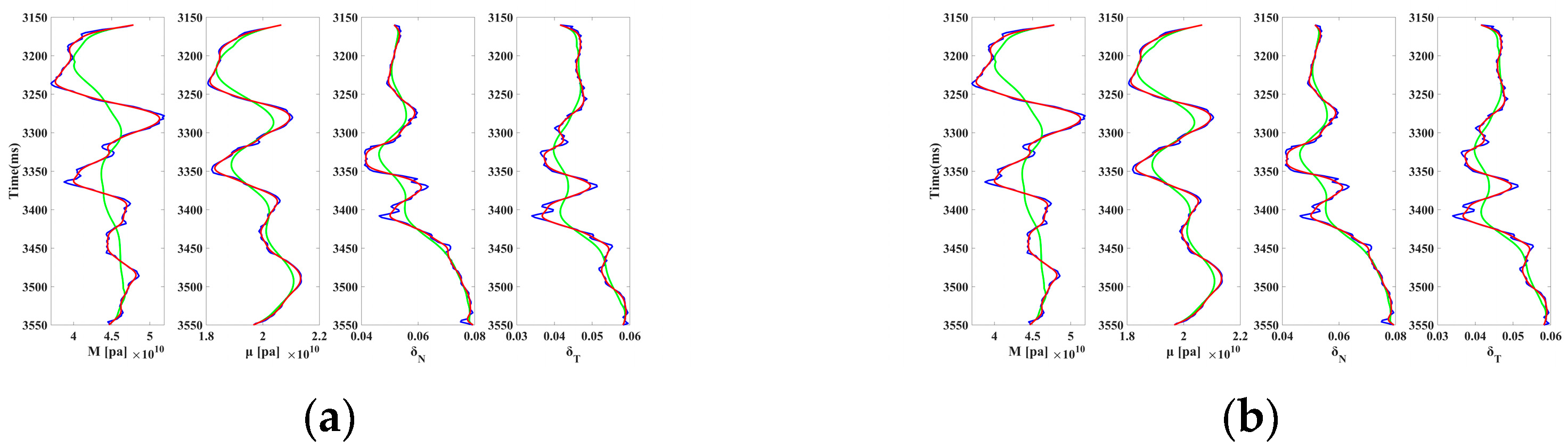
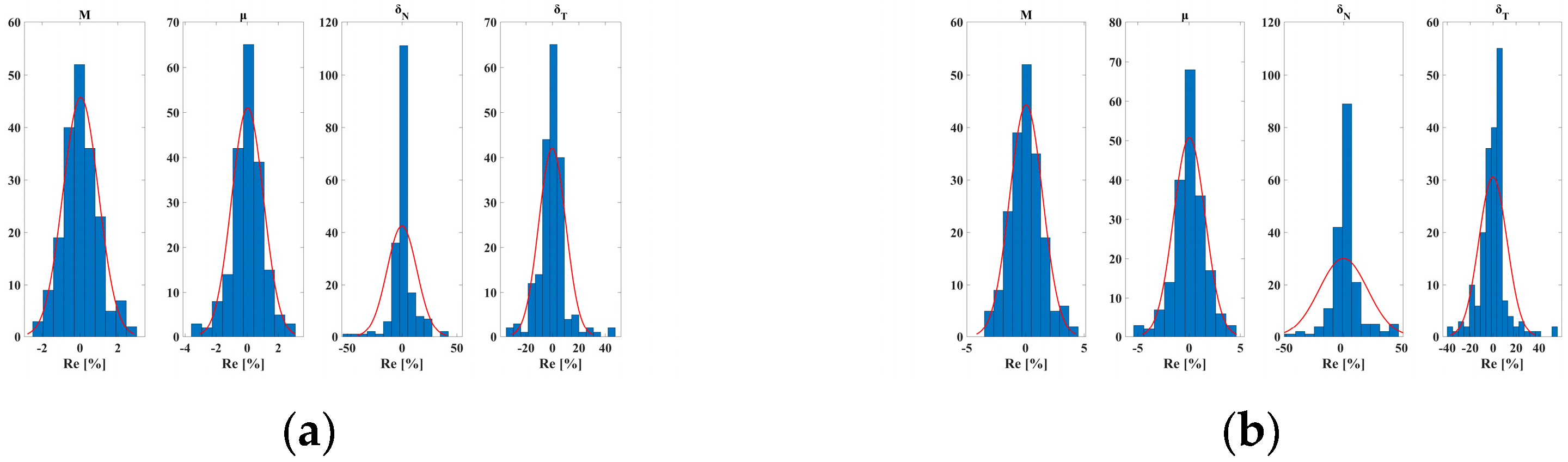
3.1. Synthetic Example

To assess the effectiveness and practicality of the proposed inversion method, a model test was conducted using data from well A, located in a basin in eastern China. Figure 4 shows the planar position of the well. Initially, key parameters such as the mineral content, pore characteristics, and anisotropy were thoroughly analyzed. Based on these parameters, a TTI petrophysical model tailored for the specific geological setting of the study area was constructed. This model was then used to compute the fracture parameter curve for the well. Next, a synthetic seismic record was generated by convolving a Ricker wavelet with a central frequency of 30 Hz and a reflection coefficient. To simulate real-world conditions and align with the methodology of Li (2022) [11], noise with a signal-to-noise ratio of two was added to the synthetic data, mimicking the interference typically observed in actual seismic recordings. Finally, the results obtained from the proposed inversion method were compared to those from a traditional inversion approach. This comparison allowed for a detailed evaluation of the advantages of the new method, particularly in terms of its ability to enhance the stability and accuracy of the inversion results.

Figure 5 presents the model test results for both the proposed inversion method and the traditional method under noise-free conditions. As shown, both methods yielded accurate inversion results without noise. Figure 6 further compares the accuracy of the two methods, with errors remaining within a reasonable range and the results appearing stable for both approaches. However, when noise is introduced, the performance diverges. Figure 7 illustrates the inversion results at a signal-to-noise ratio of two, while Figure 8 compares the associated errors. Under noisy conditions, the traditional method shows a significant decline in its fit with the logging curve, particularly for the fracture weakness parameter inversion, leading to increased errors. In contrast, the proposed method demonstrates superior stability and a notable reduction in inversion errors, especially in fracture parameter estimation, where the error is reduced by over 50%. These findings highlight the advantages of the proposed inversion method in improving the stability and accuracy of inversion, particularly for complex fractured reservoir predictions.

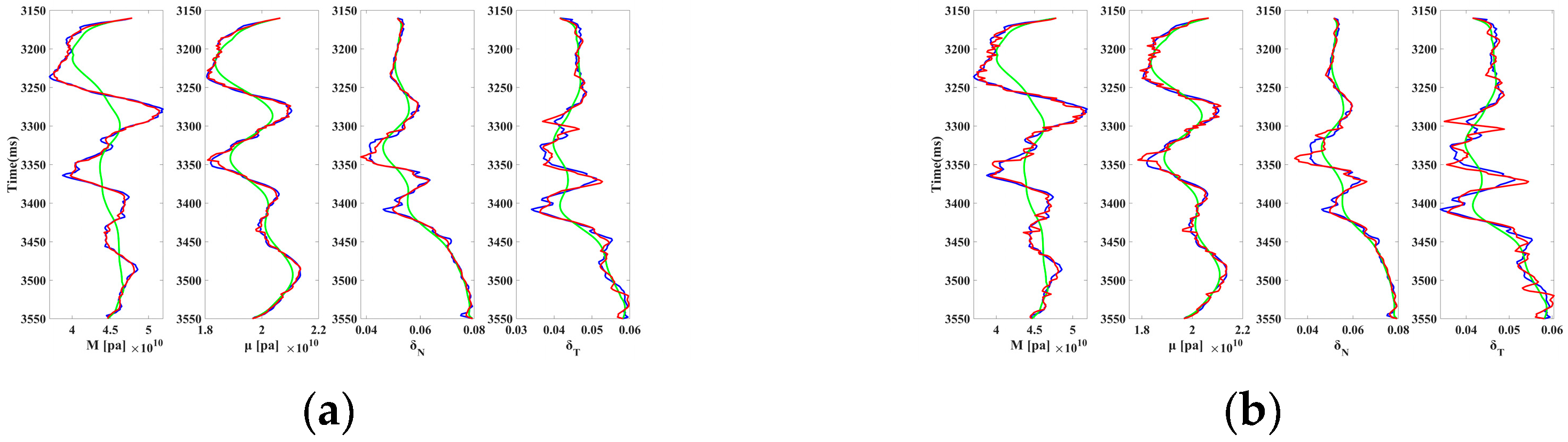
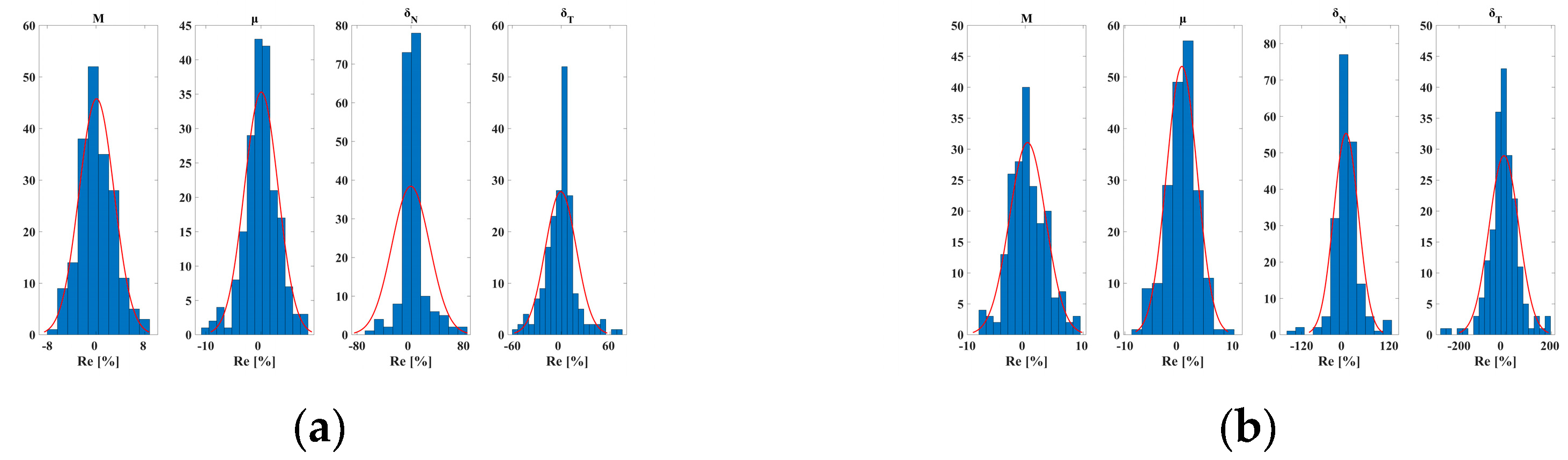
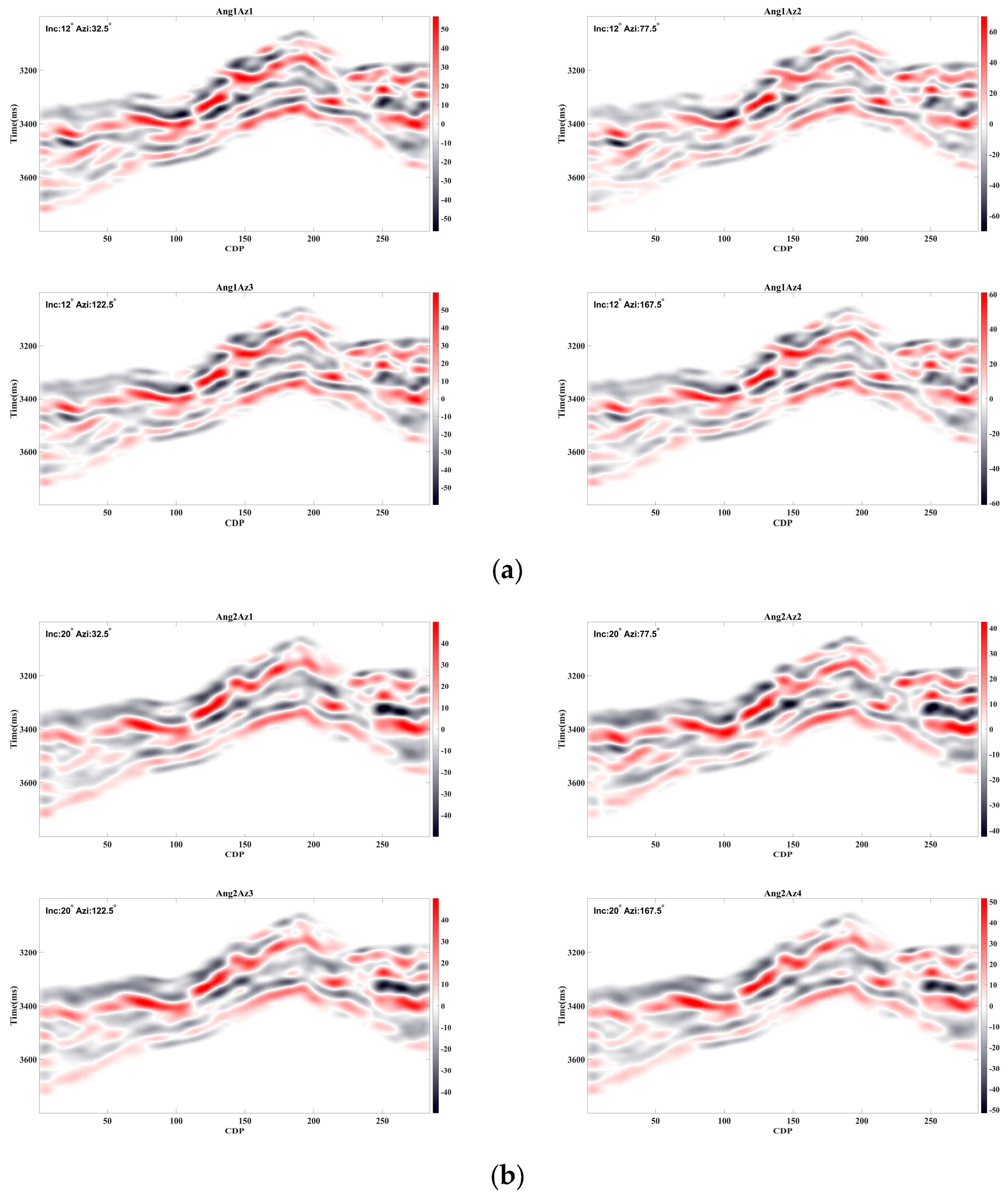
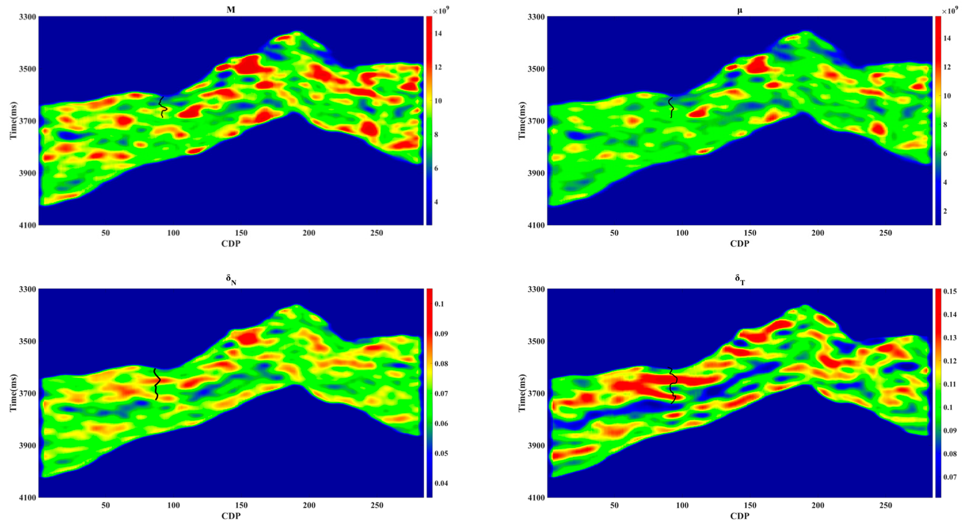
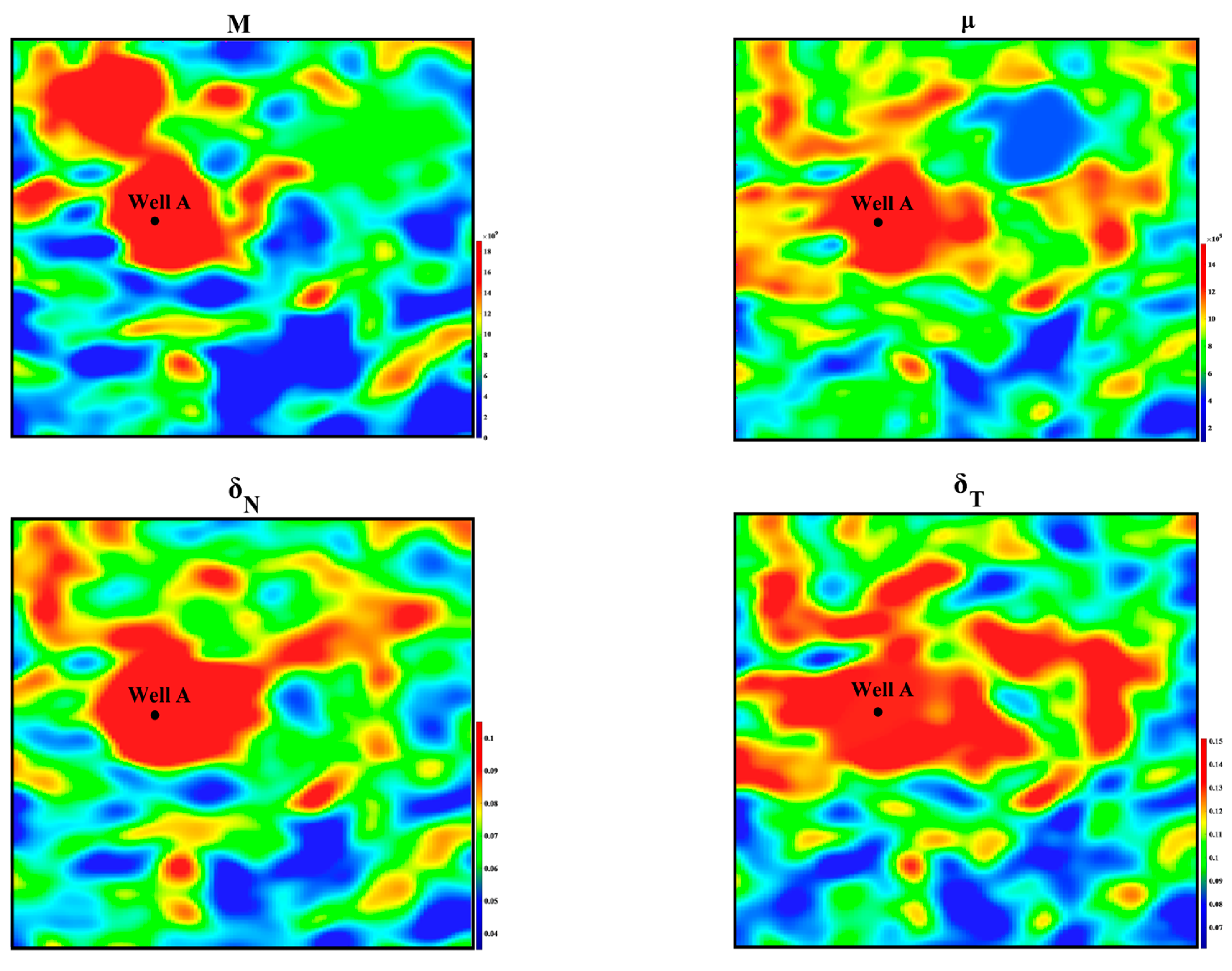
3.2. Field Data Example

The inversion method demonstrated high stability and reliability in model tests, and its application to the actual work area has yielded promising results. The violent tectonic movements in the Yanshan region, particularly since the Paleogene, have triggered frequent fractures, with the main basal faults significantly influencing fracture distribution. This has led to the development of a complex network of inclined fractures and numerous smaller fractures within the carbonate rocks, enhancing the reservoir quality and making it a high-potential target.

To improve the seismic data quality, the data in the work area were angle-stacked to increase the signal-to-noise ratio. Angle selection was based on the coverage frequency, with angles that exhibited high signal strength and extensive coverage being prioritized. The final selected incident angles were 12°, 20°, and 28°, and the azimuth angles were 32.5°, 77.5°, 122.5°, and 167.5°. The processed seismic data are shown in Figure 9.

In the data inversion process, the initial model for the parameters to be inverted was established using logging data, followed by seismic data inversion through the damping least squares method. Figure 10 presents the inversion results, which align well with the actual logging data. Specifically, the inversion results mirror the trends in the logging data for high values, which correspond to high inversion values, and low values, which correspond to low inversion values. This confirms the reliability of the inversion process.

Furthermore, the inversion results were sliced at the target layer, as shown in Figure 11. These slices indicate that the inversion results for the target horizon at well A exhibit high values, supporting their consistency with logging data interpretation. Additionally, the fracture weakness map reveals more significant fracture development in the northwest area, which is consistent with existing geological understanding. These findings validate the accuracy and robustness of the inversion results, demonstrating that the proposed reflection coefficient and inversion method are both reasonable and effective for practical application.

4. Discussions

In this study, we derive the stiffness matrix of a TTI medium with a single group of inclined fractures using the linear slip theory and the projection decomposition method. The resulting stiffness matrix consists of two components: one representing the stiffness of the background isotropic medium and the other capturing the stiffness changes induced by the inclined fractures. By applying the projection decomposition approach, the stiffness variation due to the fractures is further separated into two parts. The first component $C_{f^{\prime }}^H\sin \xi$ reflects the stiffness change in the horizontal direction, where vertical forces are less resisted, making the medium more prone to deformation. The second component $C_{f^{\prime }}^V\cos \xi$ represents the stiffness variation in the vertical direction, where horizontal forces lead to greater susceptibility to deformation.

In parameter inversion, the background isotropic medium parameters are typically expressed as the ratio of the difference to the sum of the upper and lower values, with magnitudes often around 10⁻² and occasionally 10⁻³. In contrast, fracture parameters are represented by the difference between the upper and lower values, with magnitudes generally on the order of 10⁻⁴ to 10⁻⁵ and sometimes as low as 10⁻⁶. This significant difference, up to three or even four orders of magnitude, can lead to instability in the inversion process and reduce its accuracy. Therefore, it is crucial to normalize the inversion parameters prior to the inversion to mitigate these issues and improve stability and precision. In addition, the moving mesh method can also solve some of the stability problems of fracture parameter inversion (Ivančić and Solovchuk, 2022) [7]. Since the primary focus of our paper is not on the moving mesh method, we have not delved deeply into its intricacies.

This study focuses on the TTI media model induced by a single group of inclined fractures, which is primarily applicable to inclined fracture reservoirs. Based on the paper of Hsu and Schoenberg (1993) [19], the difference between fracture weakness parameters ${\delta }_N$ and ${\delta }_T$ can serve as an indicator for fracture fluid type. Based on the findings of Ponthot and Belytschko (1998) [20], the presence of fluid influences the elastic properties of fractures, thereby altering the fracture pressure, which subsequently leads to changes in the fracture’s state. However, due to time and resource constraints, this paper does not address the fluid indicator factors. Future research can explore the inversion of these fluid factors in more detail.

5. Conclusions

This paper presents a new reflection coefficient equation for TTI media induced by a single group of inclined fractures, derived using the projection decomposition approach. Compared to previous models, the new equation demonstrates decent accuracy and rationality. To address the issue of inconsistent parameter scales during inversion, we normalized the parameters by adding and subtracting seismic data from different azimuths. One-dimensional testing using well models and actual data tests shows that the results align with both logging interpretations and geological insights from the study area, further validating its effectiveness. The findings of this study hold significant promise for practical applications in reservoir characterization, particularly in fractured reservoir exploration and development. The improved accuracy and stability of the inversion process have the potential to enhance decision-making in well placement. Finally, in the future, we will study fluid interpretation and large-scale data applications to address the shortcomings of this article.

References

1. Thomsen, L. Weak elastic anisotropy. Geophysics 1986, 51, 1954–1966. [Google Scholar] [CrossRef]
2. Rüger, A. Reflection Coefficient and Azimuthal AVO Analysis in Anisotropic Media. Ph.D. Thesis, Colorado School of Mines, Golden, CO, USA, 1996. [Google Scholar]
3. Tsvankin, I. Anisotropic parameters and P-wave velocity for orthorhombic media. Geophysics 1997, 62, 1292–1309. [Google Scholar] [CrossRef]
4. Hudson, J.A. Overall properties of a cracked solid. Math. Proc. Camb. Philos. Soc. 1980, 88, 371–384. [Google Scholar] [CrossRef]
5. Hudson, J.A. Wave speeds and attenuation of elastic waves in material containing cracks. Geophysics 1981, 64, 133–150. [Google Scholar] [CrossRef]
6. Schoenberg, M. Elastic wave behavior across linear slip interfaces. J. Acoust. Soc. Am. 1980, 68, 1516–1521. [Google Scholar] [CrossRef]
7. Ivančić, F.; Solovchuk, M. Moving mesh strategy for simulating sliding and rolling dynamics of droplets on inclined surfaces with finite element method. Comput. Methods Appl. Mech. Eng. 2022, 400, 115404. [Google Scholar] [CrossRef]
8. Bakulin, A.; Grechka, V.; Tsvankin, I. Estimation of fracture parameters from reflection seismic data—Part I: HTI model due to a single fracture set. Geophysics 2000, 65, 1788–1802. [Google Scholar] [CrossRef]
9. Chen, H.; Yin, X. Study on Methodology of Pre-Stack Seismic Inversion for Fractured Reservoirs Based on Rock Physics; China University of Petroleum: Qingdao, China, 2015. [Google Scholar]
10. Bachrach, R. Uncertainty and nonuniqueness in linearized AVAZ for orthorhombic media. Lead. Edge 2015, 34, 1048–1056. [Google Scholar] [CrossRef]
11. Li, L.; Zhang, G.; Pan, X.; Guo, X.; Zhang, J.; Zhou, Y.; Lin, Y. Anisotropic poroelasticity and AVAZ inversion for in situ stress estimate in fractured shale-gas reservoirs. IEEE Trans. Geosci. Remote Sens. 2022, 60, 5911113. [Google Scholar] [CrossRef]
12. Chen, F.; Zong, Z.; Lang, K.; Li, J.; Yin, X.; Miao, Z.; Xiao, W. Geofluid discrimination in stress-induced anisotropic porous reservoirs using seismic AVAZ inversion. IEEE Trans. Geosci. Remote Sens. 2024, 62, 5931714. [Google Scholar] [CrossRef]
13. Rüger, A. P-wave reflection coefficients for transversely isotropic models with vertical and horizontal axis of symmetry. Geophysics 1997, 62, 713–722. [Google Scholar] [CrossRef]
14. Chen, H.; Pan, X.; Ji, Y.; Zhang, G. Bayesian Markov Chain Monte Carlo inversion for weak anisotropy parameters and fracture weaknesses using azimuthal elastic impedance. Geophys. J. Int. 2017, 210, 801–818. [Google Scholar] [CrossRef]
15. Shaw, R.K.; Sen, M.K. Born integral, stationary phase and linearized reflection coefficients in weak anisotropic media. Geophys. J. Int. 2004, 158, 225–238. [Google Scholar] [CrossRef]
16. Zhang, F.; Zhang, T.; Li, X.Y. Seismic amplitude inversion for the transversely isotropic media with vertical axis of symmetry. Geophys. Prospect. 2019, 67, 2368–2385. [Google Scholar] [CrossRef]
17. Pan, X.; Li, L.; Zhou, S.; Zhang, G.; Liu, J. Azimuthal amplitude variation with offset parameterization and inversion for fracture weaknesses in tilted transversely isotropic media. Geophysics 2021, 86, C1–C18. [Google Scholar] [CrossRef]
18. Zhao, Y.; Wen, X.T.; Li, C.L.; Liu, Y.; Xie, C.L. Systematic prediction of the gas content, fractures, and brittleness in fractured shale reservoirs with TTI medium. Pet. Sci. 2024, 158, 225–238. [Google Scholar] [CrossRef]
19. Hsu, C.J.; Schoenberg, M. Elastic waves through a simulated fractured medium. Geophysics 1993, 58, 964–977. [Google Scholar] [CrossRef]
20. Ponthot, J.P.; Belytschko, T. Arbitrary Lagrangian-Eulerian formulation for element-free Galerkin method. Comput. Methods Appl. Mech. Eng. 1998, 152, 19–46. [Google Scholar] [CrossRef]
Figure 1. Classical fracture model (Chen, 2015) [9]. (a) Hudson’s penny-shaped crack model and (b) Schoenberg’s linear-slip model.
Applsci 15 02792 g001
Figure 2. Comparison of reflection coefficients: (a) the azimuth angle is 60° and (b) the incidence angle is 30°.
Applsci 15 02792 g002
Figure 3. Relative error of reflection coefficient.
Applsci 15 02792 g003
Figure 4. The location of well A.
Applsci 15 02792 g004
Figure 5. Inversion results in noise-free conditions. (a) The inversion method in this paper, and (b) the traditional inversion method. (The green line is the initial value, the blue line is the true value, and the red line is the inverted value).
Applsci 15 02792 g005
Figure 6. Inversion error in noise-free conditions. (a) The inversion method in this paper, and (b) the traditional azimuth AVO inversion method.
Applsci 15 02792 g006
Figure 7. Inversion results with S/N = 2. (a) The inversion method in this paper, and (b) the traditional azimuth AVO inversion method. (The green line is the initial value, the blue line is the true value, and the red line is the inverted value).
Applsci 15 02792 g007
Figure 8. Inversion error with S/N = 2. (a) The inversion method in this paper, and (b) the traditional azimuth AVO inversion method.
Applsci 15 02792 g008
Figure 9. The seismic data (a) and the angle of incidence are equal to 12°. (b) The angle of incidence is equal to 20°. (c) The angle of incidence is equal to 28°.
Applsci 15 02792 g009aApplsci 15 02792 g009b
Figure 10. Inversion results of model parameters.
Applsci 15 02792 g010
Figure 11. Time slice of the inversion result.
Applsci 15 02792 g011