Full-Scale Piano Score Recognition

Abstract

Sheet music is one of the most efficient methods for storing music. Meanwhile, a large amount of sheet music-image data is stored in paper form, but not in a computer-readable format. Therefore, digitizing sheet music is an essential task, such that the encoded music object could be effectively utilized for tasks such as editing or playback. Although there have been a few studies focused on recognizing sheet music images with simpler structures—such as monophonic scores or more modern scores with relatively simple structures, only containing clefs, time signatures, key signatures, and notes—in this paper we focus on the issue of classical sheet music containing dynamics symbols and articulation signs, more than only clefs, time signatures, key signatures, and notes. Therefore, this study augments the data from the GrandStaff dataset by concatenating single-line scores into multi-line scores and adding various classical music dynamics symbols not included in the original GrandStaff dataset. Given a full-scale piano score in pages, our approach first applies three YOLOv8 models to perform the three tasks: 1. Converting a full page of sheet music into multiple single-line scores; 2. Recognizing the classes and absolute positions of dynamics symbols in the score; and 3. Finding the relative positions of dynamics symbols in the score. Then, the identified dynamics symbols are removed from the original score, and the remaining score serves as the input into a Convolutional Recurrent Neural Network (CRNN) for the following steps. The CRNN outputs KERN notation (KERN, a core pitch/duration representation for common practice music notation) without dynamics symbols. By combining the CRNN output with the relative and absolute position information of the dynamics symbols, the final output is obtained. The results show that with the assistance of YOLOv8, there is a significant improvement in accuracy.

1. Introduction

Sheet music has served as the most effective method for preserving musical compositions since the classical music era of the 17th and 18th centuries, and it continues to play a crucial role today. Even in our era of advanced technology, where sophisticated recording equipment is widely available, sheet music remains an indispensable resource for musicians. However, the development of techniques for converting sheet music into computer-editable formats is a relatively recent research area within several complex domains of computer science. In recent years, researchers have introduced the concept of Optical Music Recognition (OMR), which seeks to transform sheet music images into computer-readable formats. A typical OMR workflow generally involves three primary stages: (1) Staff Line and Note Detection: Employs object detection models to remove staff lines and accurately identify the locations of musical notes. (2) Sequence Reconstruction: Utilizes recurrent neural network (RNN) models to convert note position data into sequential representations. (3) Format Conversion: Transforms the sequential data into standard formats, such as MIDI or MusicXML, using fully connected layers or autoencoders.

However, the previous approach suffers from error propagation. Errors in each step are passed on to the next, affecting the accuracy of the final result. For example, incomplete staff line removal may lead to errors in note identification, which in turn affects subsequent sequence reconstruction and encoding conversion.

Although OMR research is relatively limited, related fields such as Optical Character Recognition (OCR) have made significant progress. However, sheet music differs fundamentally from text in structure and reading rules, requiring specialized algorithms for recognition and data reorganization. Researchers like Jorge Calvo-Zaragoza [1] have developed an improved model based on Convolutional Recurrent Neural Network (CRNN) technology used in text recognition, specifically for identifying single-voice sheet music without chords. This model only requires sheet music images as input and corresponding encodings as ground truth for effective training.

In addition, most OMR research mainly focuses on basic elements of sheet music such as clefs, time signatures, key signatures, and notes, while neglecting the identification of dynamics and articulation symbols. Dynamics symbols indicate changes in volume and intensity of music, such as loud, soft, crescendo, diminuendo, etc. Articulation symbols specify how to express or play the music, such as legato, staccato, pedaling, etc. These symbols are crucial for music performers, as they greatly influence the understanding of the score and interpretation of the music. Therefore, incorporating the identification of these elements in OMR research would more comprehensively capture the complete information of sheet music.

As is well established, high-quality and moderately sized training datasets are essential for data-driven approaches. At present, no comprehensive dataset exists that includes complex-structured sheet music in bitmap format paired with corresponding computer-readable annotations. To address this gap, this study enhances the GrandStaff dataset and employs one CRNN model alongside three distinct YOLOv8 (abbr., You Only Look Once) models to convert full-page sheet music images into the KERN encoding format (KERN, a core pitch/duration representation for common practice music notation). Based on the YOLOv8 architecture, the three private models trained in our project include YOLOv8_full2single model, YOLOv8_dynam model, and YOLOv8_column model. The process begins with the YOLOv8_full2single model, which detects the positions of individual staves within the full-page sheet music image and segments the image into single-line scores based on identified coordinate ranges. Next, the YOLOv8_dynam model identifies the types, positions, and ranges of dynamics symbols in the score, subsequently removing them from the image. The third model, YOLOv8_column, determines the range of each staff line to associate the dynamics symbols with their corresponding staff lines. Finally, a CRNN model, trained on sheet music images without dynamics symbols, extracts note information and converts it into the KERN encoding format (a text-based Humdrum **kern encoding format, which is included in the Humdrum toolset [2] and is hereafter referred to simply as KERN). The results from the CRNN model are then integrated with the dynamics symbol information obtained through the YOLOv8 models, producing the final output.

The primary contribution of this research is the identification of dynamics, which has not been extensively investigated in previous studies. In classical music, dynamics play a crucial role in shaping a performer’s interpretation. Therefore, when digitizing sheet music, it is essential to include dynamics as fundamental information. Advanced Optical Music Recognition (OMR) research aims not only to convert sheet music into a computer-editable format but also, more importantly, to facilitate playback functionality. Consequently, the recognition of dynamics symbols is both necessary and critical for accurately reproducing the original performance.

2. Related Work

Baoguang Shi et al. [3] used a CRNN to recognize English text in noisy images. The CRNN first applies convolutions to the image and outputs the corresponding feature maps. The RNN then splits the feature maps into fixed-length segments and passes them through a transcript layer to merge the RNN outputs into the final string output. Similar research includes [4,5], which also attempt to use end-to-end models to recognize images containing text.

In the field of OMR, Eelco van der Wel et al. [6] used a convolutional sequence-to-sequence model to recognize single-line monophonic (without chords and one voice type) sheet music images, where each sheet music image was augmented with five different noise algorithms to generate five images. The model consists of a Convolutional Neural Network (CNN), an RNN encoder, and an RNN decoder. The sheet music images are first split into fixed-length segments before being input into different CNN blocks, then passed through the RNN encoder and RNN decoder to output the corresponding pitch and duration data (in the MusicXML encoding format).

Jorge Calvo-Zaragoza et al. [1] created the Printed Images of Music Staves (PrIMuS) dataset, which contains scanned images of single-line monophonic (without chords or voices) scores, with each image having several corresponding encoding formats, such as MEI (abbr., Music Encoding Initiative), semantic encoding, and agnostic encoding. They used this dataset to train two CRNNs, one outputting semantic encoding and the other outputting agnostic encoding. The results showed that the semantic encoding had a higher recognition accuracy.

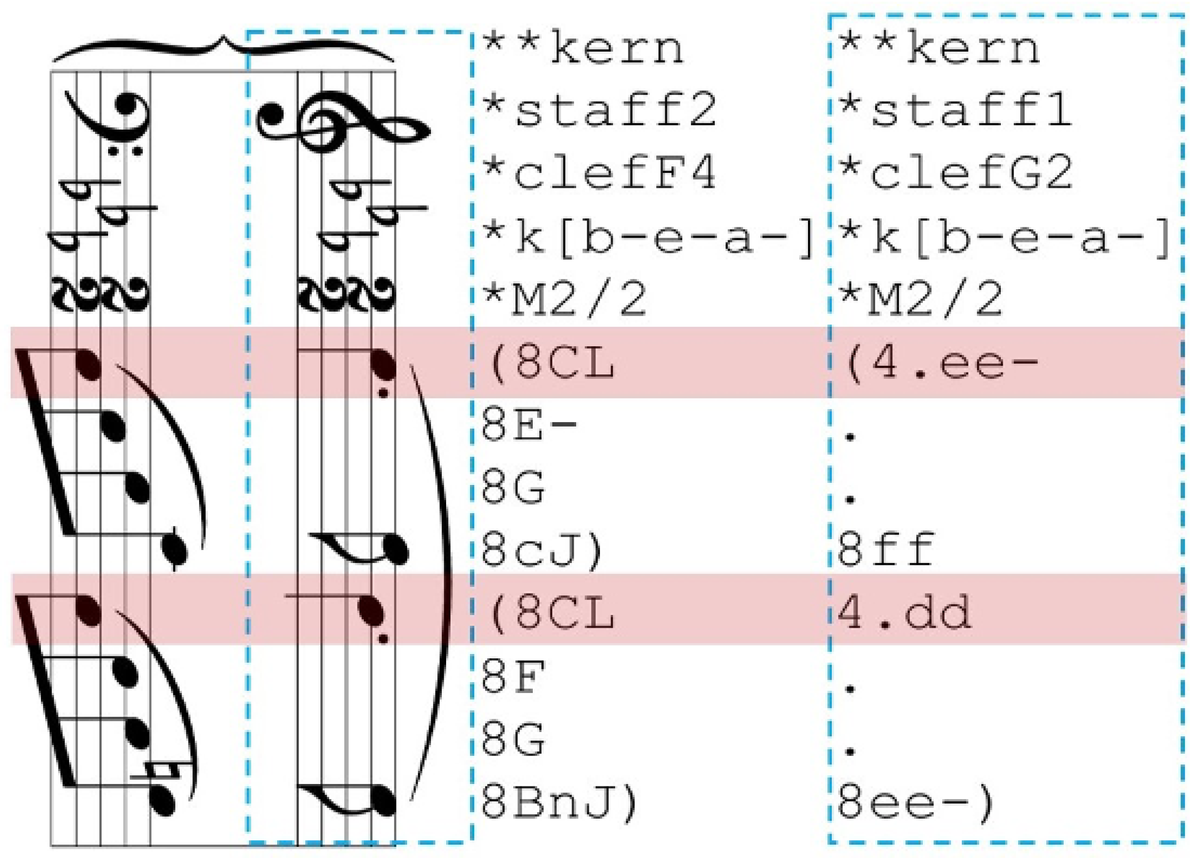
The KERN encoding format serves as a core representation of pitch and duration in common practice music notation. This format provides a text-based description of musical scores, primarily intended for computational music analysis using the Humdrum Toolkit as the principal music encoding method [2]. The KERN scheme is designed to represent fundamental musical information for Western music from the common practice period. It encodes pitch and canonical duration while also offering limited capabilities for representing accidentals, articulation, ornamentation, ties, slurs, phrasing, bar lines, stem direction, and beaming. Generally, KERN is intended to capture the underlying semantic information of a musical score rather than its visual or orthographic features, as seen in printed images. It is specifically designed for analytical applications rather than music printing or sound synthesis. This KERN music notation is among the most frequently used representations in computational music analysis. Its key features include a simple vocabulary and an easy-to-parse file structure, making it highly suitable for end-to-end OMR applications. Additionally, KERN files are compatible with dedicated music software [7,8] and can be automatically converted into other music encoding formats through straightforward operations. An illustrated example of a KERN-encoded score is presented in Figure 1. For a more detailed explanation, please refer to the official Humdrum KERN syntax documentation: https://www.humdrum.org/rep/kern/ (accessed on 20 February 2025).

Aozhi Liu et al. [9] used a Residual Recurrent CRNN (R2-CRNN) model to recognize single-line monophonic (without chords or voices) scores from the Camera-PriMuS dataset, with and without distortion noise. The sheet music images were converted into feature maps by multiple CRNNs and then passed through an RNN to output both semantic and agnostic encoding formats. Antonio Rios-Vila et al. [10] used the SEILS Dataset and CAPITAN Dataset and employed a CRNN to recognize full-page monophonic scores, converting them to the MEI format. The SEILS dataset consists of black-and-white scanned images from 16th-century Italian madrigals, while the CAPITAN dataset contains color images of handwritten scores from the 17th century. Both datasets have simpler structures compared to modern scores.

The research in [11,12] utilized end-to-end models to recognize more complex sheet music images, including homophonic music (which includes chords but no vocal lines) and polyphonic music (which contains both chords and vocal lines). However, developing a sufficiently general model that can handle various levels of score complexity continues to pose a challenge.

In the research [12], the authors utilize the GrandStaff dataset and employ a CRNN as the model for identifying notes. However, unlike the study [12], our research aims to identify dynamics, which do not exist in GrandStaff. Therefore, we augment the KERN encoding with randomly positioned crescendo, decrescendo, and dynamics symbols. Meanwhile, our research employs the YOLOv8 model to assist in identifying these dynamics symbols. The function of YOLOv8 is to identify the type and position of dynamics symbols and combine this information into the KERN encoding output by the CRNN.

In the study [13], Antonio Rios-Vila et al. used a CRNN and a CNNT (Convolution Neural Network Transformer) to recognize single-line piano scores. An innovative aspect of their work was the use of a reshape layer in the CRNN to segment the notes and convert them to the corresponding KERN format using an RNN or transformer. The results showed that the CNNT outperformed the CRNN when provided with more data.

Furthermore, in the paper [14], Arnau Baró et al. trained a CRNN on standard sheet music-image data and then performed transfer learning on the trained model using handwritten sheet music images. The results showed a recognition accuracy of 90% for handwritten scores.

3. Method

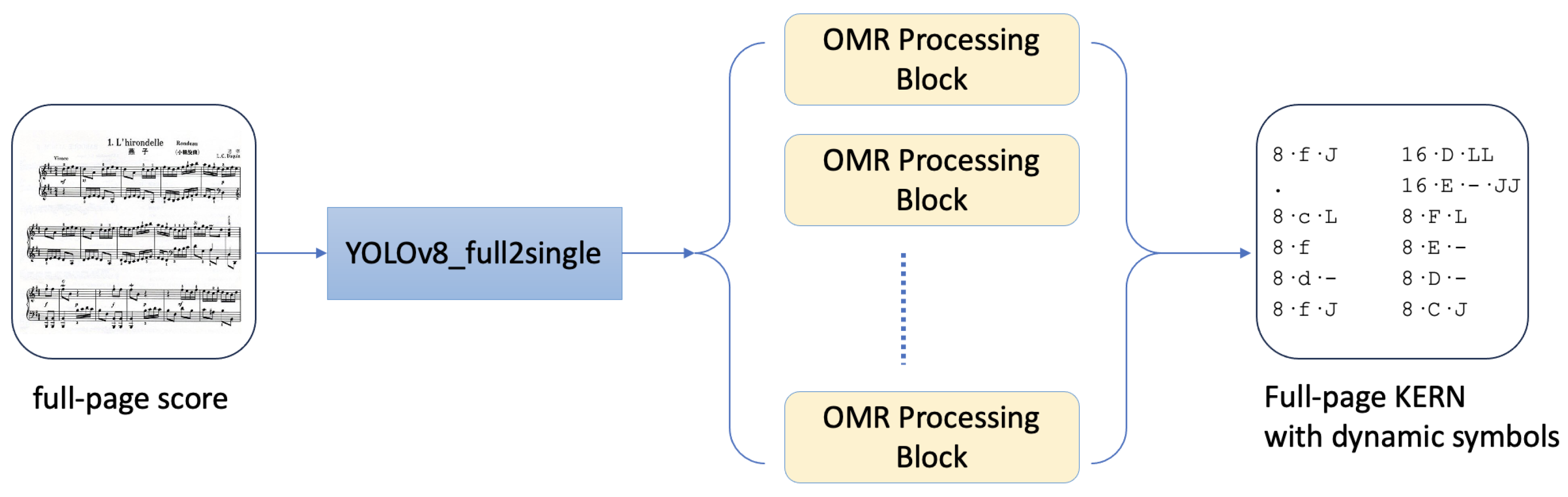
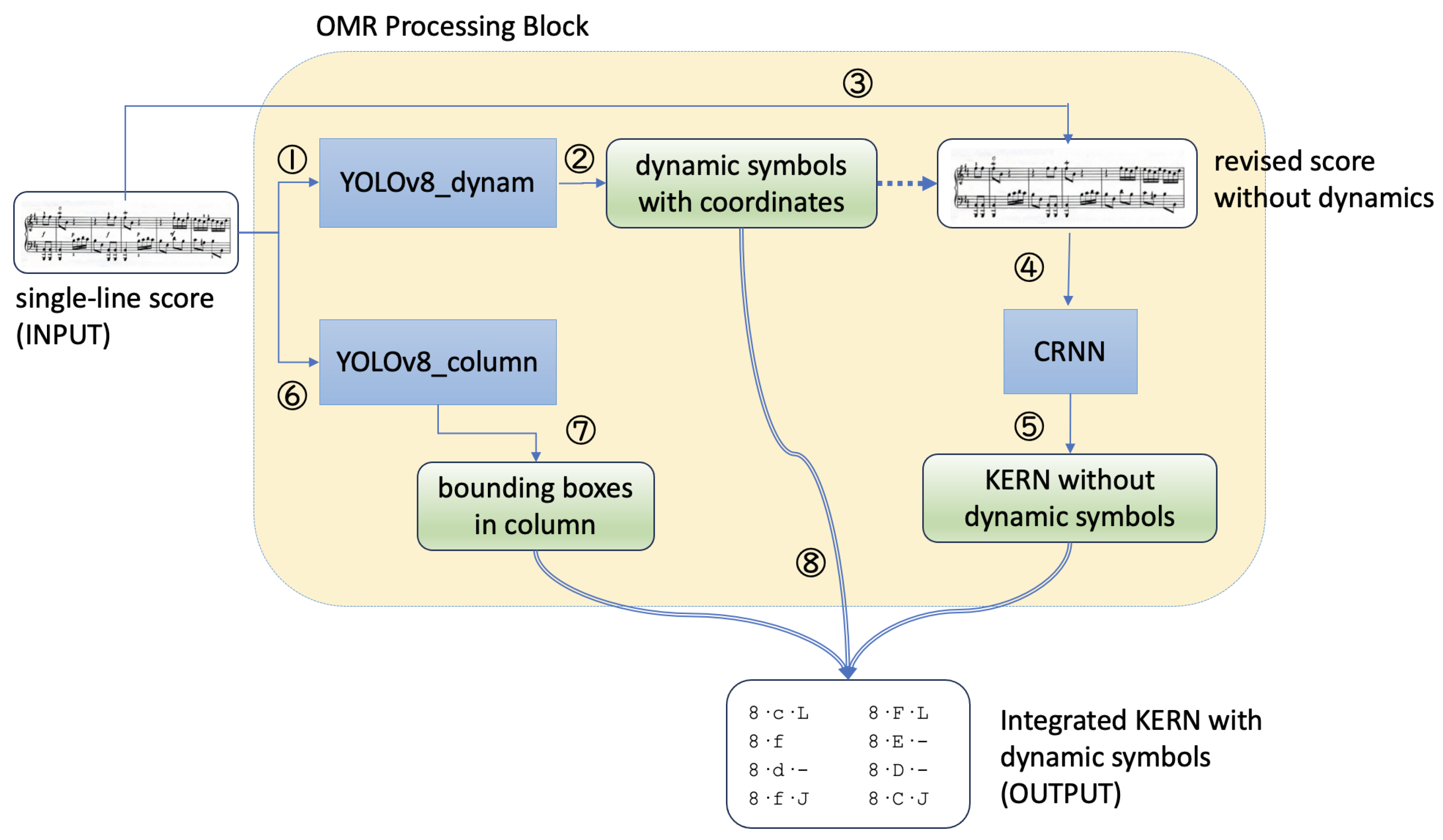
The overall model architecture is illustrated in Figure 2, in which the OMR processing block is detailed in Figure 3. The process begins with the input of a full-page score, which is processed by the YOLOv8_full2single model to segment it into multiple single-line scores. Each segmented single-line score is then passed through two additional models: YOLOv8_dynam and YOLOv8_column. YOLOv8_dynam identifies all dynamics symbols, while YOLOv8_column detects all staff lines, enabling the integration of dynamics information into the KERN encoding.

Once YOLOv8_dynam detects the dynamics symbols, it removes them from the score image. The modified image, along with the corresponding KERN file (excluding dynamics symbols), is subsequently input into the CRNN for training. The KERN encoding predicted by the CRNN is then combined with the dynamics symbol types, positional information, and staff line details to produce a complete score that incorporates dynamics symbols.

This process is repeated for each single-line score segmented by YOLOv8_full2single, with each score generating its own KERN encoding. The individual KERN encodings are then sequentially merged to form the final complete encoding.

3.1. Find Dynamics via YOLOv8

Before training the CRNN on sheet music, it is crucial to detect and remove dynamics symbols, as their presence can negatively impact the accuracy of note recognition. As outlined in the data augmentation section, the positions and ranges of the dynamics symbols are extracted from the SVG file, while their types and sequences are derived from the KERN file.

The training dataset comprises 43,105 image samples, with 5389 samples designated for both testing and validation. The dataset includes 12 categories of dynamics symbols: f, p, mf, mp, fp, ff, pp, sf, cre, $dec$, $cre\_word$, and $dec\_word$. For YOLOv8 training, these categories are mapped to numerical labels ranging from 0 to 11. Specifically, the symbols $cre$, $dec$, $cre\_word$, and $dec\_word$ correspond to the top-left, top-right, bottom-left, and bottom-right symbols in Figure 4, respectively. Each symbol is enclosed within a bounding box to support YOLOv8 training.

Before training the YOLOv8 model, certain parameters must be modified to disable the image-flipping function. By default, YOLO applies image mirroring during training; however, flipping the $cre$ and $dec$ symbols would entirely alter their meanings.

Compared to other models, YOLOv8 achieves faster convergence during training while maintaining high accuracy in various object detection tasks. As a result, utilizing the YOLOv8 model not only enhances performance but also provides greater flexibility for future research developments.

This paper [15] mentions that in image segmentation tasks, YOLOv8 outperforms Mask R-CNN in terms of both accuracy (Precision and Recall) and inference time. Therefore, we consider YOLOv8 to be a more scalable and adaptable choice. According to the YOLO documentation (available at https://docs.ultralytics.com/zh/models/yolov8/#supported-tasks-and-modes, accessed on 17 July 2024), a performance comparison of different YOLO model versions is provided. The results indicate that YOLOv8 exhibits significantly higher accuracy and lower latency compared to other models, including YOLOv7, YOLOv6-2.0, and YOLOv5-7.0.

In this study, most parameters of YOLOv8 remained unchanged, except for two key modifications:

• Dropout: This parameter was set to $0.2$ (default: 0), meaning that in each neural network layer, there is a $20\%$ probability of randomly deactivating neurons, which helps reduce overfitting.
• flipud, fliplr: These parameters control the probability of YOLOv8 flipping images either upside down (flipud) or left-right (fliplr) during training. Since sheet music images contain sequential information, flipping them would disrupt the reading order, leading to a complete alteration of musical content. To preserve the integrity of the data, both parameters were set to 0.0.

After YOLOv8 detects the positions and ranges of the dynamics symbols, they are removed from the sheet music images. This is accomplished using the Python PIL package (accessible at https://pypi.org/project/pillow/, accessed on 17 July 2024) by replacing all pixels within the bounding box regions with white.

3.2. Find Staff Column via YOLOv8

To reconstruct the removed dynamics symbols into the KERN file, it is necessary to determine their original positions within the score. The position of each dynamics symbol is calculated by identifying the corresponding bounding box in which the symbol is located. Figure 5 illustrates an example of bounding boxes of notes within a column. In this figure, the image contains 26 bounding boxes and four dynamics symbols: f located within the 1st box, $dec$ spanning from the 9th to the 15th box, mf in the 20th box, and mp in the 23rd box.

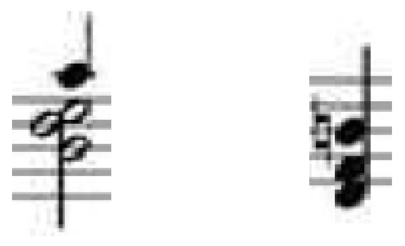
To identify each bounding box, objects with the “notehead” tag in the SVG file are analyzed, and the x and y coordinates of the notes within these objects are extracted. It is important to note that chords containing two notes separated by an interval of a second may be mistakenly recognized as two distinct notes due to their proximity. To address this issue, the “chord” tag is utilized to group all “notehead” child objects under a single entity. Figure 6 provides examples of scenarios with and without chords containing seconds.

3.3. CRNN Structure

Convolutional-Recurrent Neural Network (CRNN) is a model that uses a Convolutional Neural Network (CNN) as an encoder and a Recurrent Neural Network (RNN) as a decoder. The encoder first outputs a feature map, which is then sliced and concatenated into a sequence of feature vectors. The decoder converts this feature vector into the target text form. In this study, a CNN is used as the encoder and an RNN as the decoder.

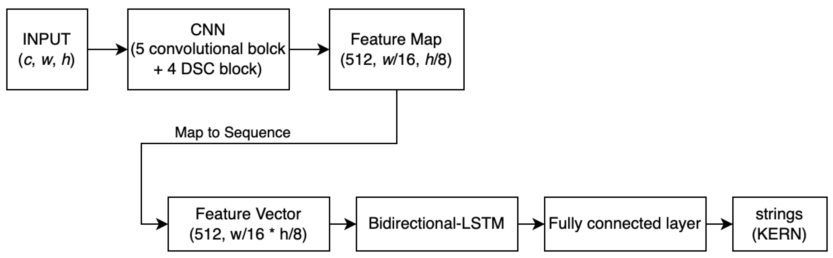
Assuming the input image size is (c, h, w), where c represents the number of channels, h represents the height, and w represents the width, the CRNN architecture (shown in Figure 7) consists of the following:

• Convolutional Layers: This layer transforms the input image into a feature map of size (512, $w/16$, $h/8$). Then, through a reshape layer, the feature map is converted into a two-dimensional feature vector of size (512, $(w/16)\ast (h/8)$).
• Recurrent Layers: The feature vector output by the Convolutional Layers is passed through a Bidirectional LSTM to generate an output vector. Finally, a fully connected layer transforms this output vector into the final text output.

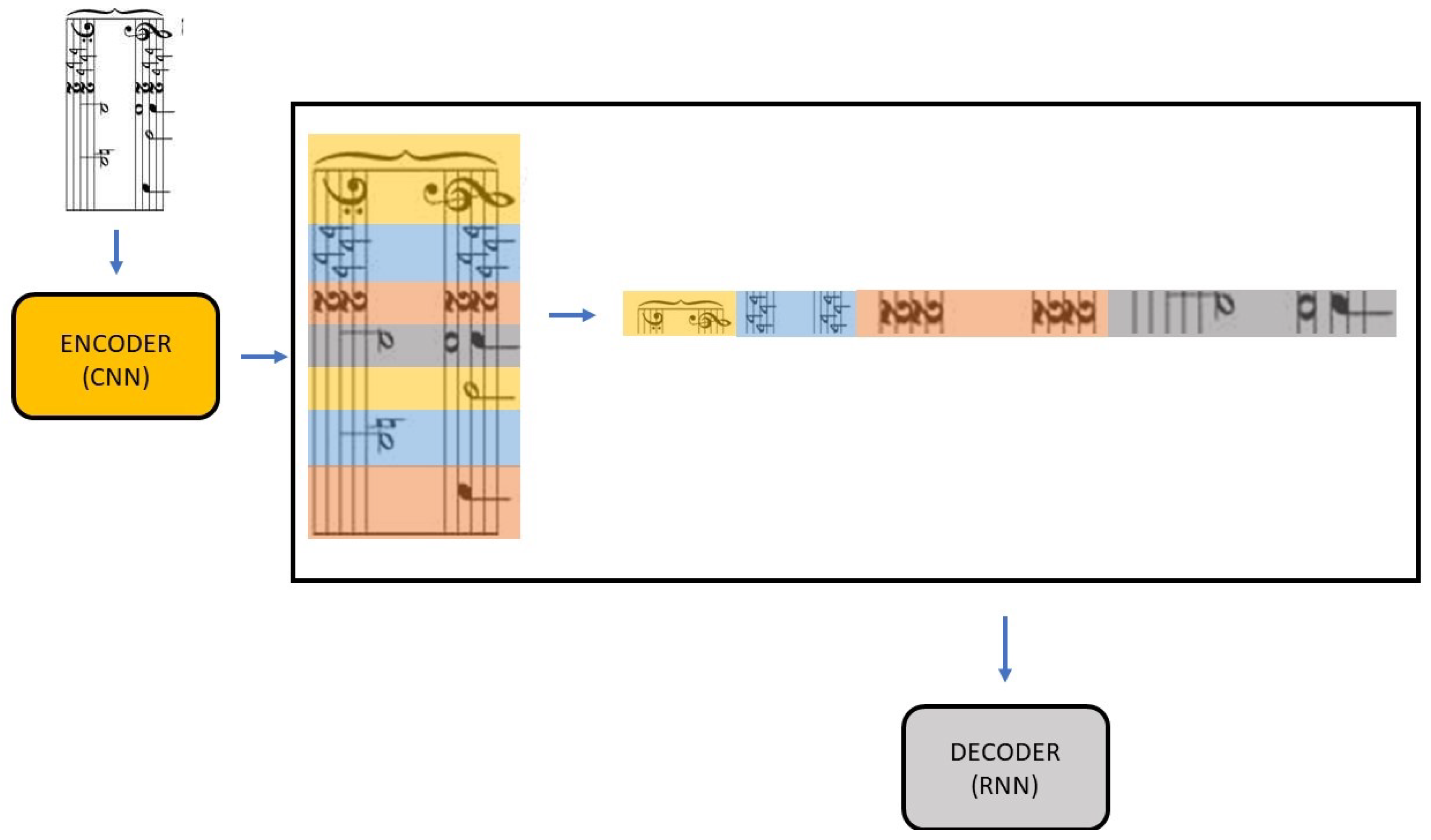
Figure 8 illustrates a method for converting multi-voice sheet music into target text. This method involves several steps:

• Input the multi-voice sheet music image into the CNN.
• The CNN extracts relevant features from the input image, transforming it into a feature map.
• Slice all rows of the feature map and concatenate them into a long sequence of feature vectors.
• The concatenated image sequence is passed to the RNN.
• The RNN’s output is converted into the final text output (KERN encoding) through vocabulary projection.

It is important to note that the image concatenation step occurs in the feature space extracted by the encoder, not directly on the input image pixels. The visualization in Figure 8 is provided for better understanding. This method can transcribe multi-voice sheet music without explicit staff line segmentation.

3.4. CTC Loss Function

The OMR aims to find the most likely label $\widehat{s}$ for each image x, where $\widehat{s}$ is encoded from the vocabulary set ${\sum }_a$.

$$\widehat{a}=arg\underset{s\in {\sum }_a}{max}P\left(s\right|x)$$

(1)

The model is trained using Connectionist Temporal Classification (CTC) loss [16] to approximate this probability. The CTC formula is as follows:

$$P\left(s\right|x)=\sum _{a\in As,x}\prod _{t=1}^T{p}_t\left(a_t\right|x)$$

(2)

$A_{s,x}$ is a set containing all possible labels a. For an input x, we need to calculate the probability of x being predicted as each a, and find the maximum value. ${\prod }_{t=1}^T{p}_t\left(a_t\right|x)$ represents that x is divided into T frames, each of these frames is converted into a label $a_t$, and a probability $p_t\left(a_t\right|x)$ is obtained. Multiplying these probabilities gives the probability of one type of a. There are many combinations of a that can be predicted, and we need to sum these probabilities to get the probability of predicting $\widehat{a}$ given an x. Moreover, CTC adds a blank character $ϵ$ to ${\sum }_a$, allowing the model to predict blank labels. The vocabulary set with the blank character is called ${\sum }_a^{\prime }$. $\widehat{a}$ may contain many blank characters and repeated characters. Therefore, through the function $\mathcal{B}(.)$, consecutive identical characters in $\widehat{a}$ are reduced to one and blank characters are removed, to obtain the final predicted character $\widehat{s}$.

$$\widehat{s}=\mathcal{B}\left(\widehat{a}\right)$$

(3)

In summary, the model’s processing can be summarized in the following two mathematical expressions:

$$\begin{array}{c}\hfill \widehat{a}=arg\underset{\widehat{a}\in {\sum }^{\prime }}{max}\prod _{t=1}^{T}P\left(a_t\right|x).\widehat{s}=B\left(\widehat{a}\right)\end{array}$$

(4)

4. Dataset

The objective of this research is to recognize full-page piano sheet music containing dynamics symbols and convert it into a computer-readable encoding format. The dataset utilized in this study is derived from the GrandStaff dataset [17], which comprises 53,882 classical piano sheet music fragment images (single-line) along with their corresponding encoding files in the KERN format. The collection features works by composers such as Ludwig van Beethoven, Wolfgang Amadeus Mozart, and Frédéric Chopin. The sheet music is rendered using Verovio [18], a music notation engraving library.

However, the GrandStaff dataset does not include full-page piano sheet music, nor does it contain dynamics symbols. As a result, the data augmentation meets the requirements of this research. This section details the data augmentation techniques employed to address these limitations. Section 4.2 explains the methodology for incorporating dynamics symbols into the single-line scores, while Section 4.3 describes the processes of image erosion and dilation to simulate the characteristics of scanned sheet music.

4.1. Concatenate Single-Line Score to Full-Page Score

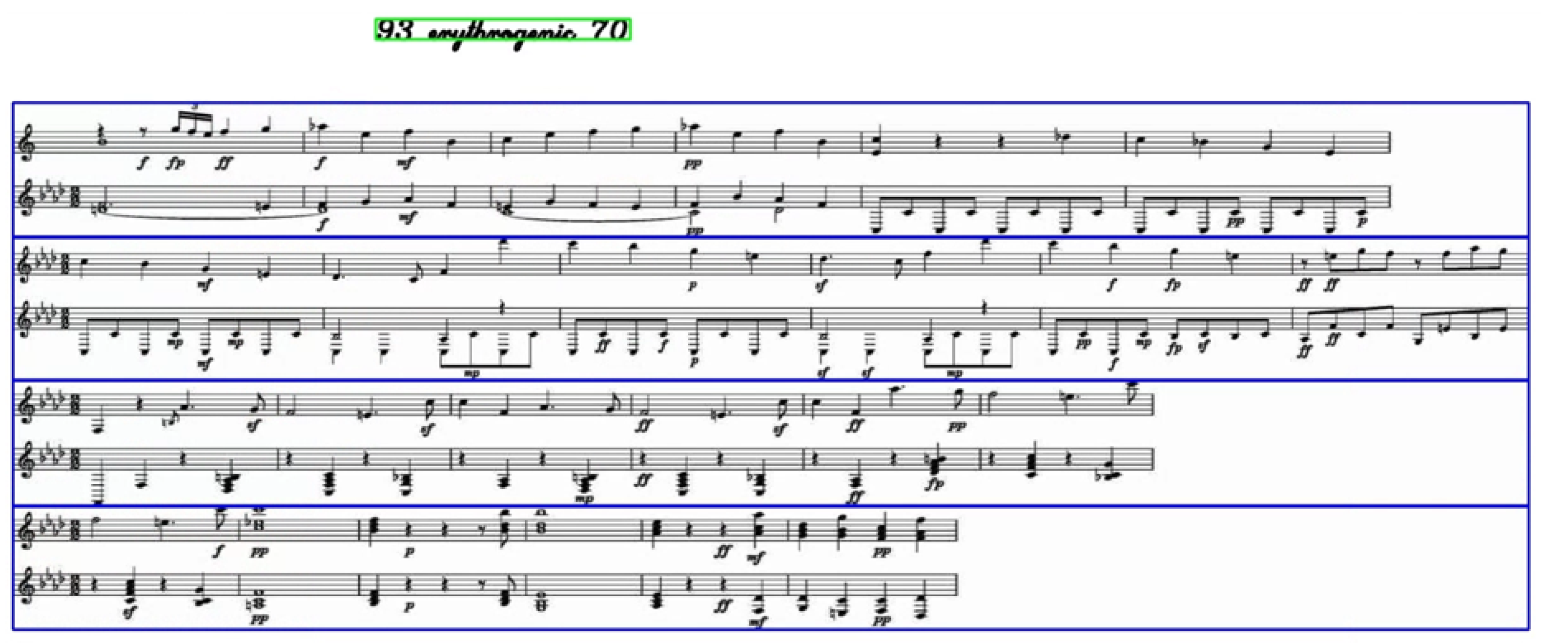
To create a full-page music score image with four lines, four single-line music score images are vertically concatenated, as illustrated in Figure 9. Following the concatenation, random text and numbers are added to the top of the image to simulate the titles, authors, and other information typically found at the top of sheet music. Each concatenated music score line is labeled as “staff”, while the text at the top of the image is labeled as “words”, with their respective bounding box coordinates serving as ground truth for training the YOLOv8 model.

4.2. Add Dynamics Symbols to Single-Line Score

The GrandStaff dataset includes information such as clefs, key signatures, time signatures, and notes; however, it lacks dynamics symbols and articulation symbols, which are essential elements in classical music. To address this limitation, we add these symbols to enrich the dataset. Dynamics symbols are incorporated into each KERN file, with their positions and types selected randomly. 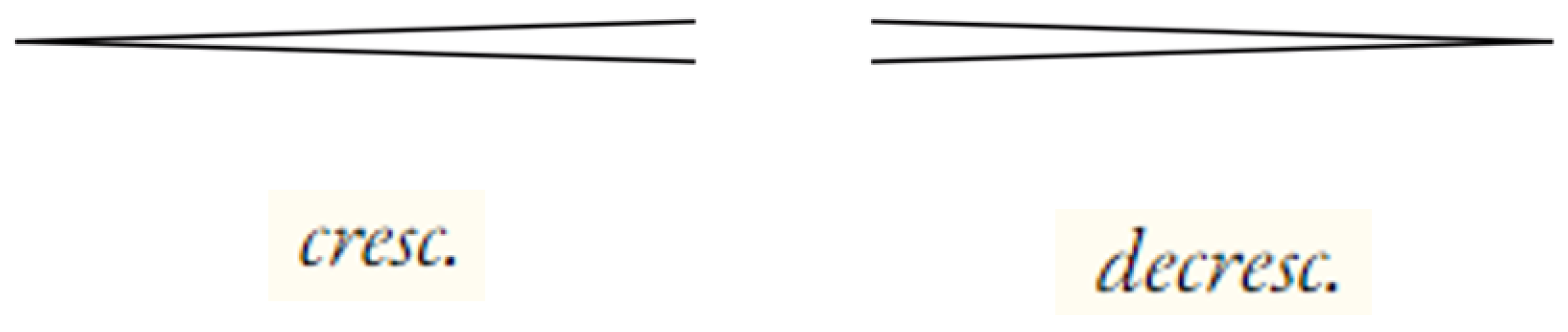The types of dynamics symbols include f, p, mf, mp, fp, ff, pp, and sf, comprising a total of eight types. In addition to short-structured dynamics symbols, we also introduce long-structured dynamics symbols. Figure 4 illustrates examples of long-structured dynamics symbols commonly used in classical sheet music.

To generate a music score with dynamics symbols, we randomly insert symbols based on estimated probabilities. We augment the KERN encoding with randomly positioned crescendo, decrescendo, and dynamics symbols. In the KERN encoding, the probability of adding dynamics symbols to each row is as follows: 4% each for f, p, mf, and mp; 3% each for ff, pp, fp, and sf; and 72% for not adding any dynamics symbols. There are four types of crescendo and decrescendo symbols: cre and dec (< and >) each account for 40%, while cre_word and dec_word each account for 10%. The details on the number of dynamics symbols added are specified in

Table 1. Dynamics symbols and their numbers.

Dynamics Symbol	Number				Dynamics Symbol	Number
f	33,306				pp	17,474
p	30,725				sf	14,690
mf	34,978				cre	19,035
mp	29,769				dec	16,048
fp	17,122				cre word	5258
ff	15,902				dec word	5184

.

Note that the GrandStaff dataset is a corpus comprising 53,882 printed images of single-line pianoform scores, along with their digital score encoding in the form of KERN transcriptions. It includes both original works from six authors in the Humdrum repository and synthetic augmentations of the music encodings, enabling a greater variety of musical sequences and patterns for music analytic applications [19].

In the study by [19], the authors introduce the Sheet Music Transformer, the end-to-end OMR model designed to transcribe complex musical scores without relying exclusively on monophonic strategies. The proposed model has been evaluated using the GrandStaff dataset. However, within this dataset, only core pitch and canonical duration information are encoded, while dynamics symbols are not included.

Meanwhile, our research focuses on the identification of dynamics, in addition to core pitch and canonical duration information. However, it is unnecessary to construct an entirely new dataset from scratch. By leveraging the existing GrandStaff dataset, we incorporate dynamics symbols to create a comprehensive dataset for our model development and performance evaluation.

4.3. Apply Image Erosion and Dilation to Score

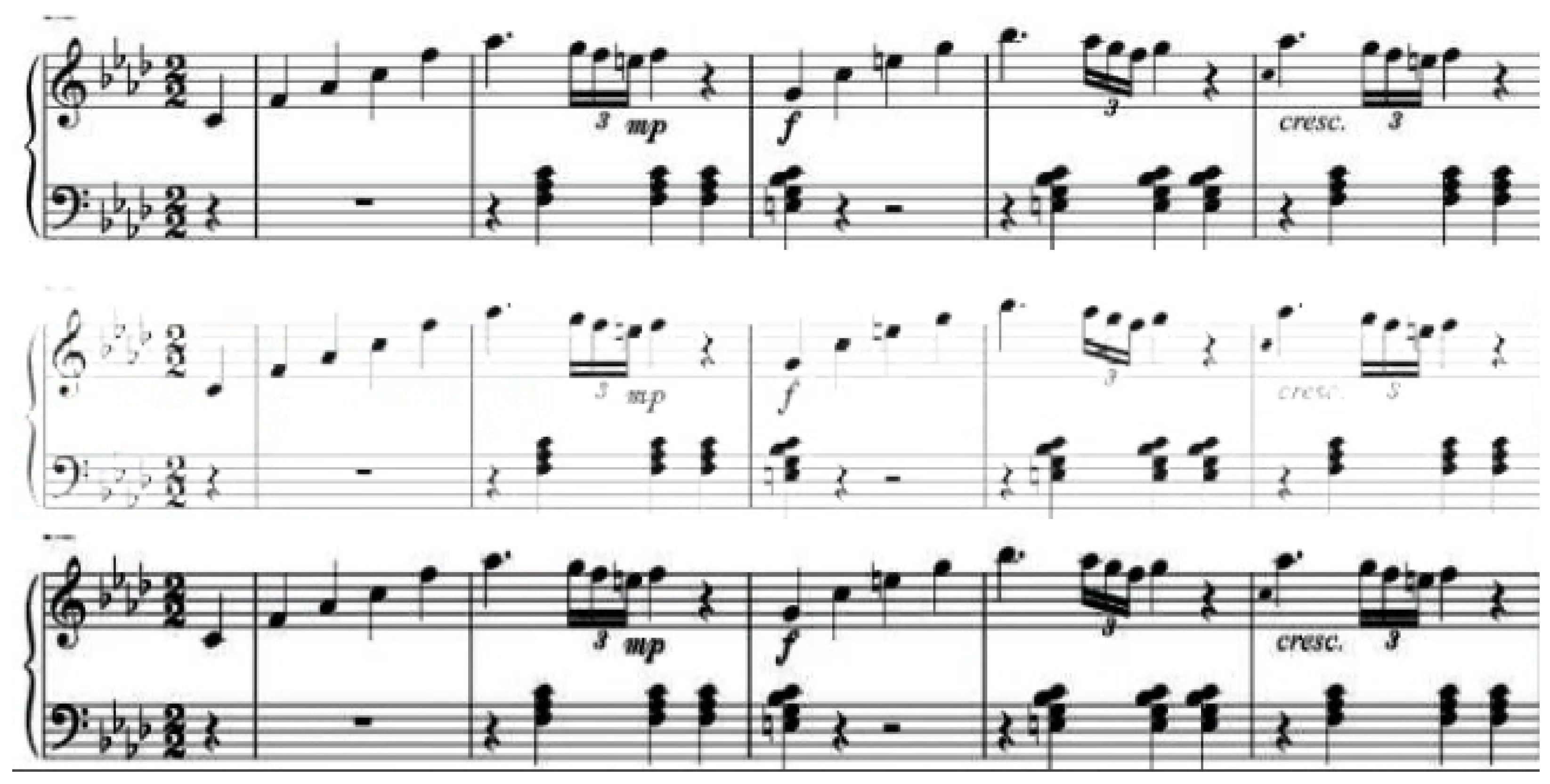
In addition to training on standard images, it is crucial to account for the characteristics of scanned sheet music, as most sheet music images available online are digitized from physical scores. These scanned scores often exhibit erosion or dilation artifacts. In eroded images, bar lines may appear thinner, and diagonal lines, such as ties, may become jagged. Conversely, in dilated images, closely positioned elements may overlap—for instance, accidentals merging with adjacent notes or the beams of 16th and 32nd notes intersecting. If the model is trained exclusively on standard sheet music, it may struggle to accurately recognize scanned scores affected by erosion or dilation. Therefore, it is necessary to artificially generate training data that simulates these effects. Based on the GrandStaff dataset, our dataset also includes images generated through erosion and dilation, maintaining equal proportions and quantities. Specifically, the ratio of eroded to dilated images is 1:1, with 26,941 eroded images and 26,941 dilated images.

Figure 10 illustrates the eroded and dilated images utilized in this study. These images were generated using the Python library cv2.

5. Evaluation

The model’s output is a new KERN encoding. To compare it with the ground truth and obtain accuracy, we used the following method:

$$\mathcal{E}(\widehat{S},S)={\displaystyle \frac{{\sum }_{i=0}^{n}d(s_i,{\widehat{s}}_i)}{{\sum }_{i=0}^n\left|s_i\right|}}$$

(5)

where S is the ground truth dataset, $\widehat{S}$ is the dataset predicted by the model, and $\mathcal{E}(\widehat{S},S)$ is the distance between sets $\widehat{S}$ and S. $d(s_i,\widehat{s_i})$ is the distance between the ground truth data and predicted data in the i-th sample, and $|s_i|$ is the length of the i-th sample. The value of $d(s_i,\widehat{s_i})$ depends on the definition of a token. The first is Character Error Rate (CER), which considers a single character as a token. The second is Symbol Error Rate (SER), which treats an entire KERN symbol as a token. The third is Line Error Rate (LER), which considers a KERN row as a token. For YOLOv8, four evaluation criteria are used: Precision, Recall, mAP50, and mAP90-95.

$$\mathrm{Precision}={\displaystyle \frac{\mathrm{TP}}{\mathrm{TP}+\mathrm{FP}}}$$

(6)

$$\mathrm{Recall}={\displaystyle \frac{\mathrm{TP}}{\mathrm{TP}+\mathrm{FN}}}$$

(7)

$$\mathrm{mAP}50={\displaystyle \frac{1}{N}}\sum _{i=1}^N\mathrm{AP}i$$

(8)

$$\mathrm{mAP}50\text{-}95={\displaystyle \frac{1}{10}}\sum _{r=[0.5:0.05:0.95]}\mathrm{AP}\mathrm{at}\mathrm{IoU}=r$$

(9)

Precision and Recall are evaluation methods for detected object classes, while mAP50 and mAP50-95 are for bounding boxes. Precision is the proportion of samples predicted as positive by the model that are actually positive in the ground truth. Recall is the proportion of positive samples in the ground truth that are predicted as positive by the model. In the mAP50 formula, the numerator is the sum of AP for all classes. The denominator is the number of classes N. Therefore, a higher mAP50 value indicates higher average precision across all classes. In the mAP50-95 formula, the numerator is the sum of AP for all classes at IoU thresholds from 0.5 to 0.95, with an interval of 0.05. The denominator is 10, which is the number of IoU threshold values from 0.5 to 0.95. Therefore, a higher mAP50-95 value indicates higher average Precision across all classes over the range of IoU thresholds from 0.5 to 0.95.

6. Result

This section presents the performance analysis of four models in the following sequence: (1) YOLOv8 accuracy for dynamics symbols; (2) Bounding box detection accuracy; (3) CRNN accuracy; (4) Overall model accuracy.

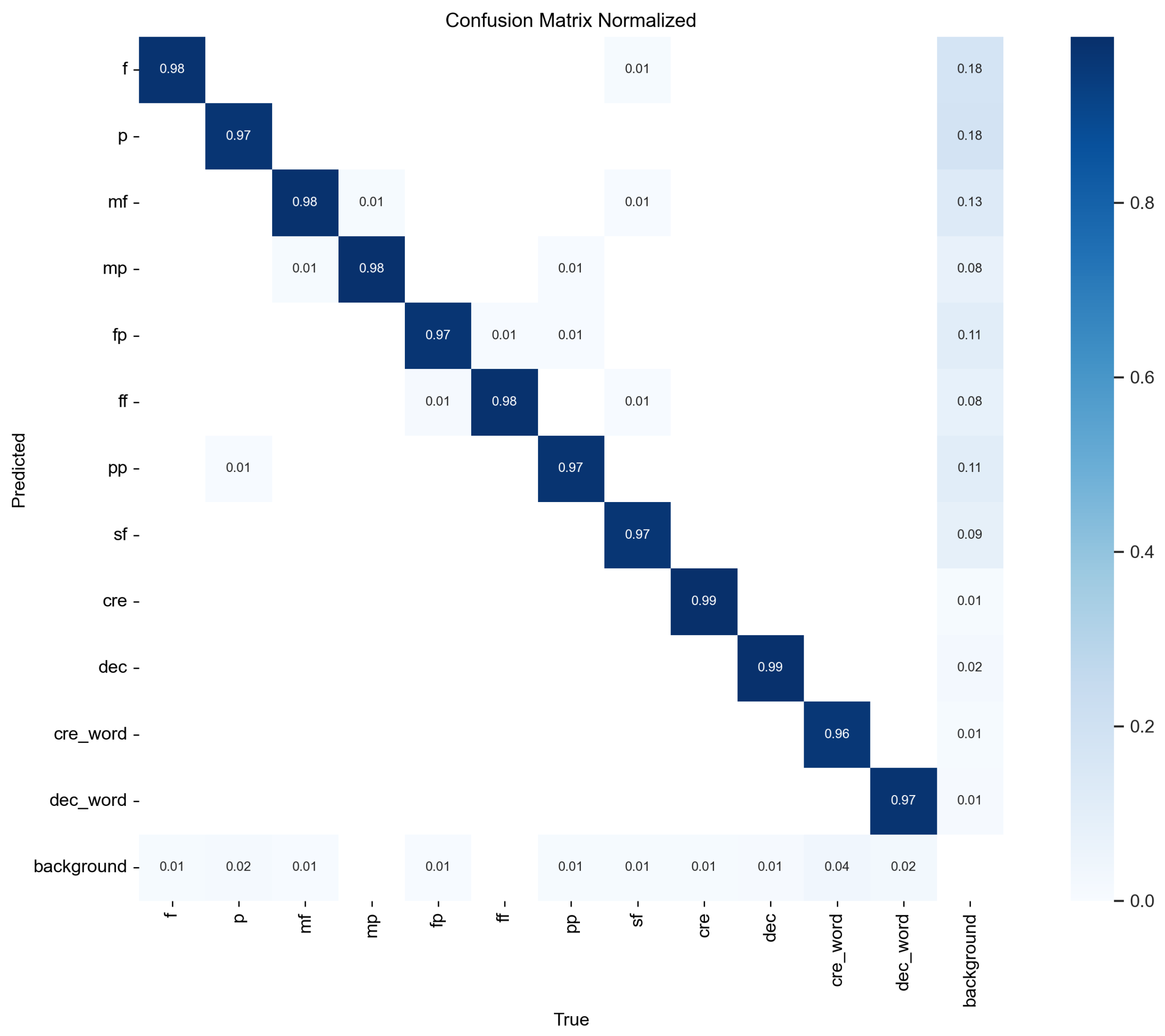
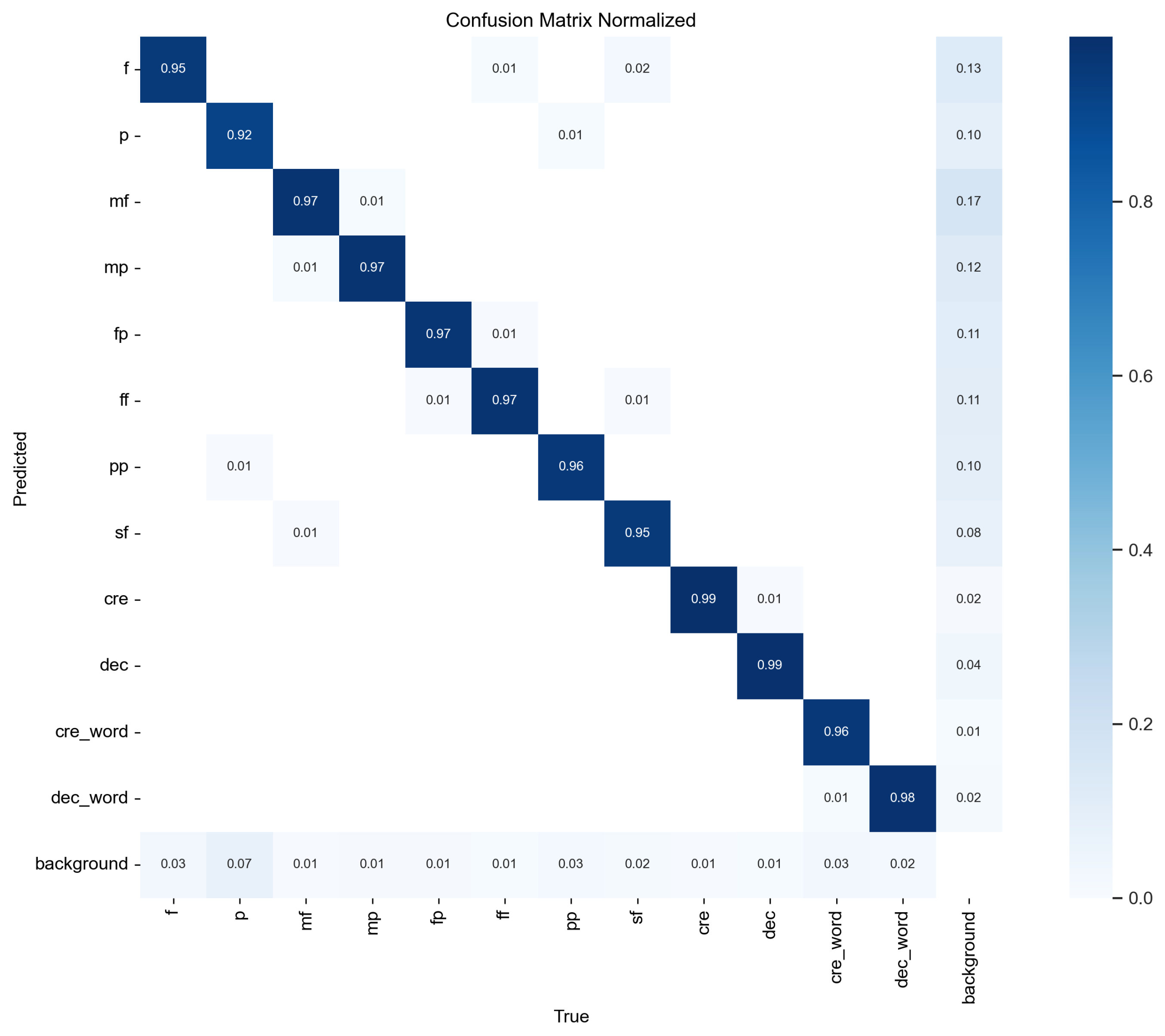
Figure 11 and Figure 12 show confusion matrices illustrating YOLOv8’s accuracy on dynamics symbols, with results for both original images and images that have undergone erosion or dilation. YOLOv8 demonstrates strong performance in recognizing the types and positions of dynamics symbols, although the mAP50-95 score is slightly lower—approximately 0.86 for character-type dynamics symbols and around 0.8 for long-structure dynamics symbols. This discrepancy is likely due to the smaller number of long-structure dynamics symbols. However, in this study, even when the bounding box is slightly larger, as long as it does not overlap with the note information (i.e., the notes are not whitewashed), it does not significantly impact the CRNN’s ability to recognize dynamics symbols.

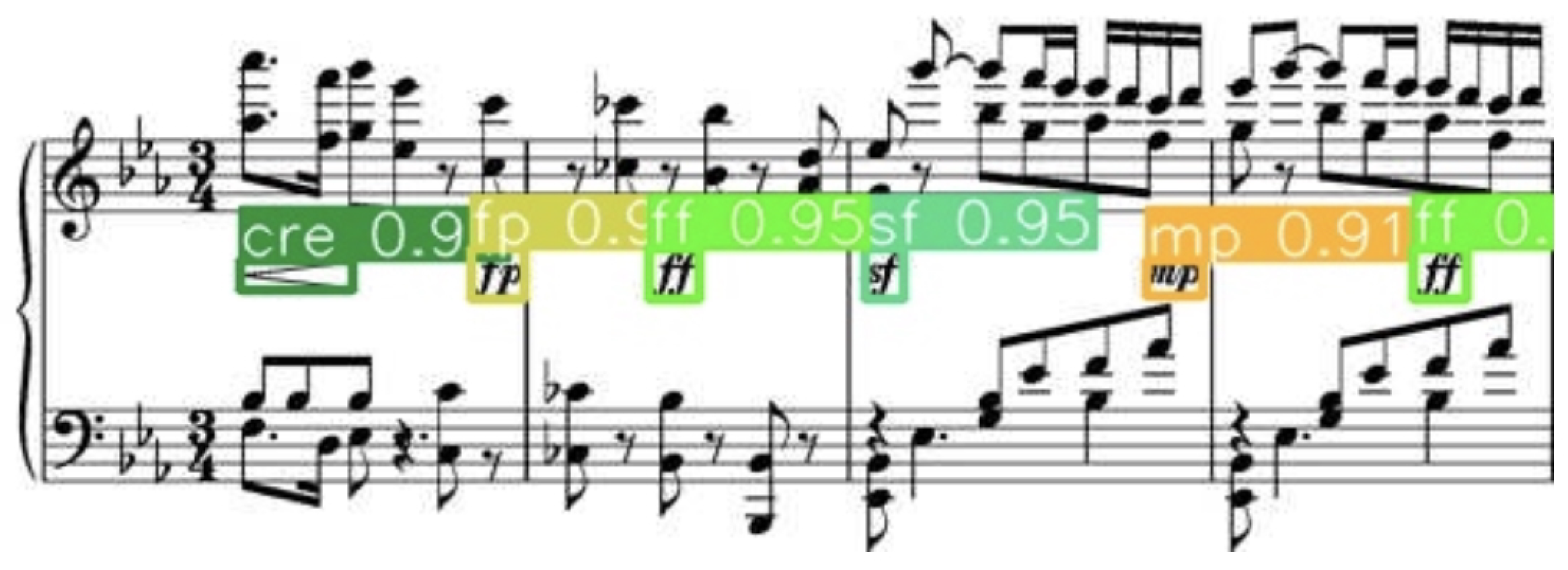
Figure 13 presents examples of dynamics symbols detected by the YOLO model. The value next to the class name indicates YOLOv8’s confidence level for each object class and the corresponding bounding box. As shown in Figure 13, YOLO’s prediction of the coordinates and range of dynamics symbols is highly accurate, with confidence levels consistently exceeding 0.9. Therefore, the removal of dynamics symbols has little to no effect on the accuracy of note information.

From the confusion matrix in Figure 11 and Figure 12, we observe minimal differences in the results between images with erosion/dilation and normal images in terms of distinguishing dynamics symbols, further underscoring YOLOv8’s robustness in recognizing dynamics symbols.

Table 2. Accuracy of YOLOv8 for image column position. Top: Accuracy for the original image. Bottom: Accuracy for eroded or dilated images.

Type	Images	Instances	Precision	Recall	mAP50	mAP50-95
original	5389	185423	0.994	0.988	0.995	0.937
erosion_dilation	5389	185939	0.991	0.988	0.995	0.924

shows YOLOv8’s accuracy in detecting bounding boxes. The purpose of this model is to combine the positions of dynamics symbols with the KERN file output by CRNN, rather than using the original CRNN. This is because long-structure dynamics symbols are poorly recognized within CRNN and may even affect the output of the note section, so the design of separate models is suggested for recognition. In addition,

Table 3. The performance of object classification.

Class	Images	Instances	Precision	Recall	mAP50	mAP50-95
all	1212	6060	0.988	0.982	0.990	0.840
staff	1212	4848	0.994	0.997	0.995	0.959
words	1212	1212	0.983	0.968	0.985	0.721

shows the YOLOv8’s performance of object classification.

Table 2 primarily explores the analysis of data for datasets without and with dynamics symbols when using CRNN, as well as CRNN in conjunction with YOLOv8. It also examines the differences in model performance on normal and eroded or dilated image data. The main findings of Table 2 include the following:

• Comparing normal sheet music images with eroded or dilated sheet music images (normal, erosion dilation tables), the latter has slightly higher error rates than the former, as expected. Since many datasets in previous studies have used images with noise and image shifts, this study also includes this data.
• For rows CRNN+YOLOv8 for no dynam and CRNN+YOLOv8 for dynam(in both normal and eroded or dilated), the CER and SER are similar. However, there is a difference in LER, indicating that YOLOv8 has a low error rate in identifying dynamics symbols (YOLOv8_dynam), but has more error rate in identifying sheet music column (YOLOv8_column).
• For rows CRNN+YOLOv8 for no dynam and CRNN for no dynam, the error rates are very close, indicating that YOLOv8 does not identify positions without dynamics symbols as having dynamics symbols.
• When identifying sheet music images containing dynamics symbols, CRNN paired with YOLOv8 (CRNN+YOLOv8 for dynam) has a significantly lower error rate than CRNN without YOLOv8 (CRNN for dynam). This highlights the necessity of YOLOv8 for processing dynamics symbols.

Table 4. Top: CER, SER, LER for original images without and with dynamics symbols using only CRNN and CRNN combined with YOLOv8. Bottom: CER, SER, LER for eroded and dilated images without and with dynamics symbols using only CRNN and CRNN combined with YOLOv8.

normal	CER	SER	LER
CRNN for no dynam	3.52	5.12	13.80
CRNN+YOLOv8 for no dynam	3.63	5.24	14.05
CRNN for dynam	8.43	14.23	42.34
CRNN+YOLOv8 for dynam	3.85	5.76	29.70
erosion dilation	CER	SER	LER
CRNN for no dynam	6.55	10.70	30.60
CRNN+YOLOv8 for no dynam	6.72	10.83	30.74
CRNN for dynam	9.40	15.65	45.85
CRNN+YOLOv8 for dynam	6.80	11.25	42.49

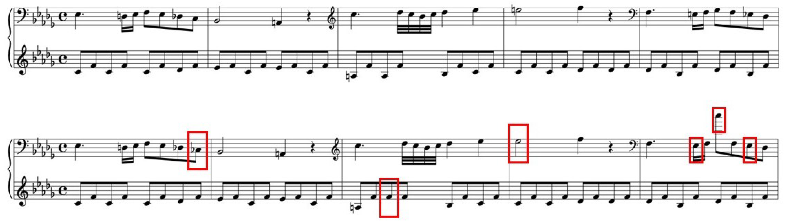
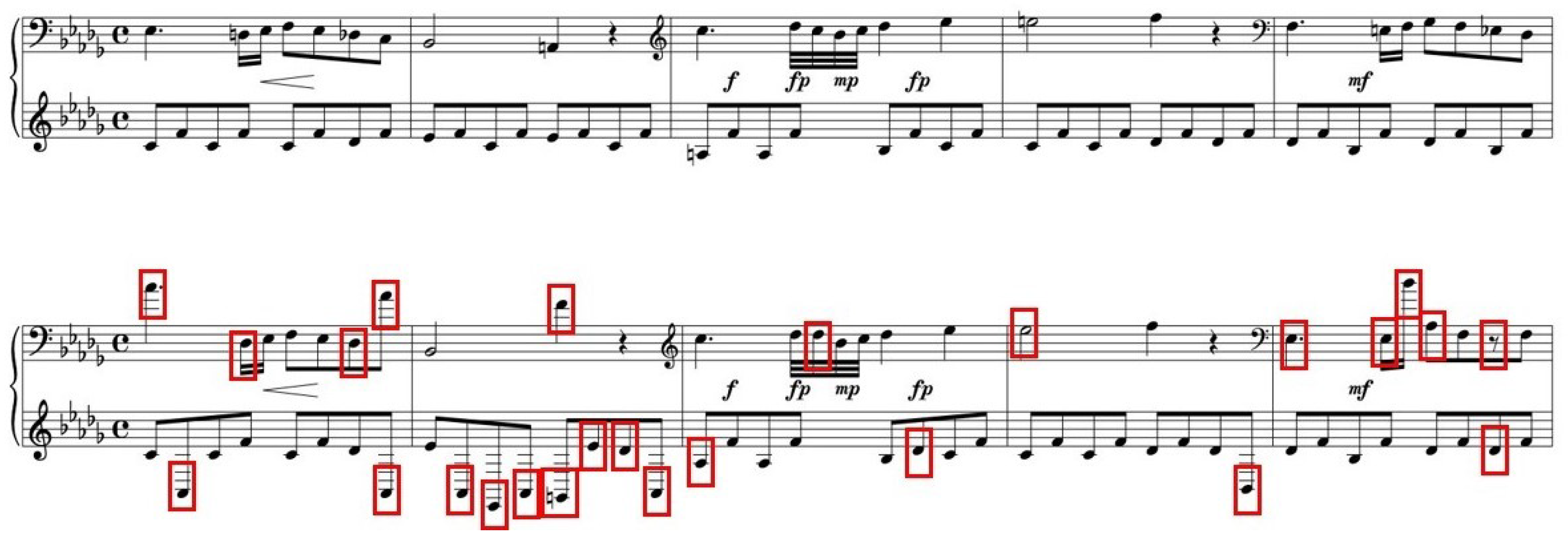
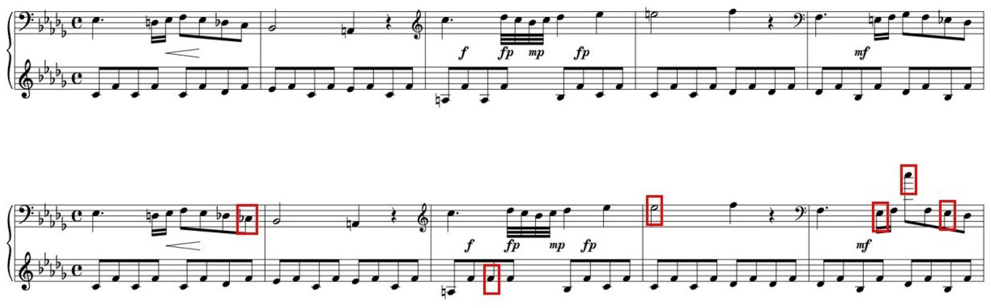
shows the error rates for CRNN and CRNN with YOLOv8 on test data for original images (with or without dynamics symbols), eroded and dilated images (with or without dynamics symbols). Figure 14 and Figure 15 show images rendered by Verovio from KERN files output by CRNN for sheet music images without and with dynamics symbols, respectively, along with their ground truth sheet music images. Figure 16 shows the combination of CRNN and YOLOv8 outputs, along with the ground truth. 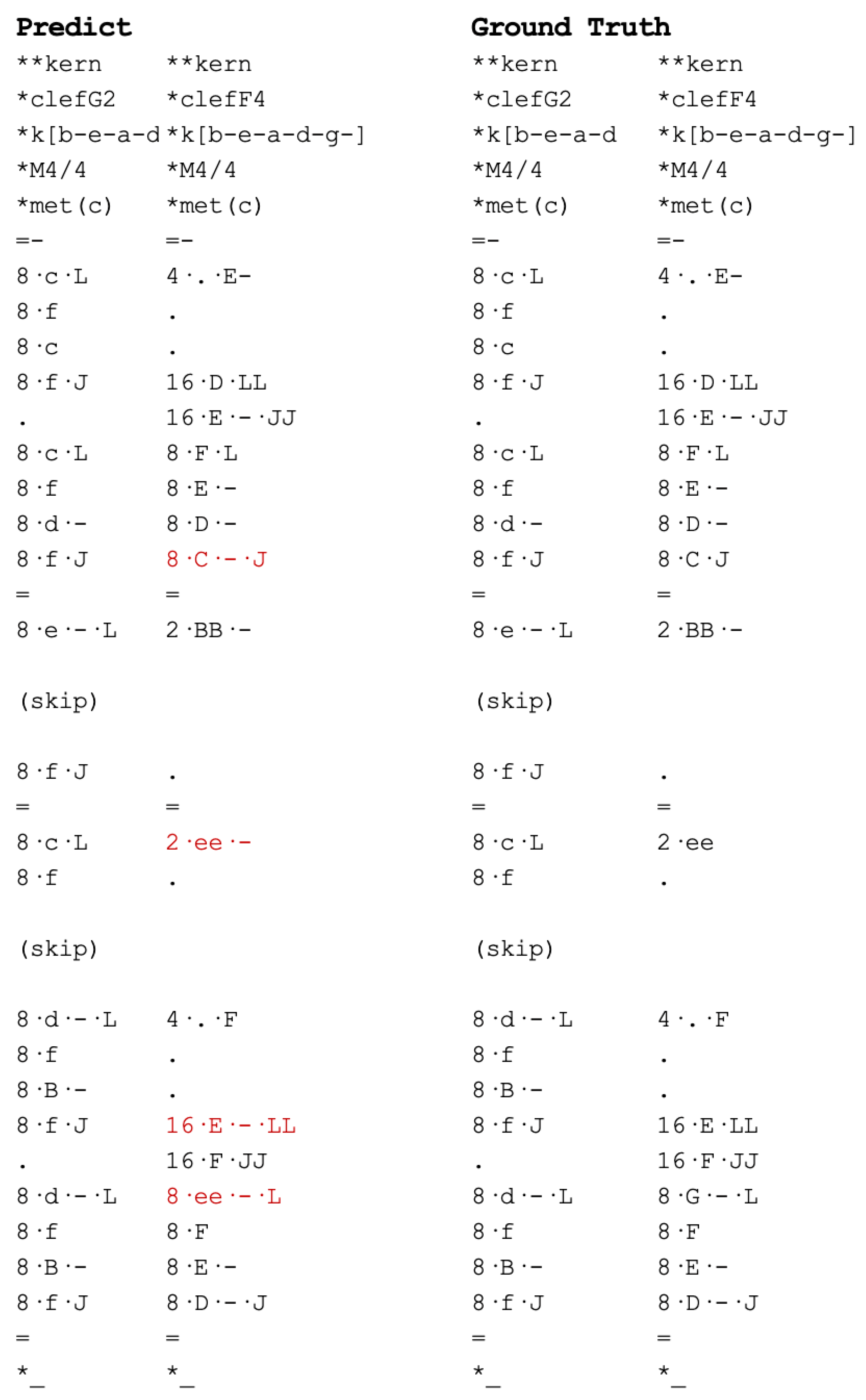Figure 17 shows a comparison between the KERN encoding generated by CRNN and the ground truth.

In Figure 14, Figure 15 and Figure 16, the ‘red squares’ indicate the resulting errors. A detailed discussion is provided below. Figure 14 shows the results of CRNN recognition of sheet music images without dynamics symbols. As we can see, except for the last measure where one note is significantly higher than the ground truth pitch, the remaining errors are mostly due to missing sharps, flats, or naturals, but the notes themselves are not incorrect.

Figure 15 shows the results of CRNN recognition of sheet music images with dynamics symbols. It can be seen that the errors in the recognition results are significantly more than those in Figure 14, and almost all incorrectly recognized notes differ greatly in pitch from the ground truth. Interestingly, the CRNN itself is very accurate in recognizing dynamics symbols, but the recognition of notes becomes very poor. From this, it can be inferred that the model may have overfitting problems when the CRNN is used to simultaneously recognize different types of objects.

Figure 16 shows the recognition results of CRNN combined with YOLOv8 for sheet music images containing dynamics symbols. Because the CRNN reuses the model from Figure 14, which recognizes sheet music without dynamics symbols, and YOLOv8 demonstrates powerful capabilities in recognizing dynamics symbols, the results are very good.

In the comparison between Figure 14 and Figure 15, it can be observed that the latter has lower accuracy for notes but high accuracy for dynamics symbols. The former, in the absence of dynamics symbols, has much higher accuracy for the note section compared to the latter. This indicates that CRNN excels at processing sheet music with only note information, but when both notes and dynamics symbols are present, the accuracy for notes decreases significantly. Therefore, the dynamics symbol part needs to be handled by YOLOv8.

From Figure 15 and Figure 16, we observe that because CRNN no longer needs to process dynamics symbols, the accuracy for notes greatly improves, and YOLOv8 can effectively output the positions of dynamics symbols and bounding boxes, thereby accurately combining dynamics symbol information back into the KERN encoding.

This study focuses on the identification of dynamics symbols, a topic not addressed in previous research, thereby making direct comparisons with prior work challenging. When only considering simple OMR without dynamics symbols, the comparison still remains challenging because of no benchmark. In

Table 5. The performance of OMR in error rate of paper [13]. (Note that the “Camera GrandStaff” uses GrandStaff for base and adds distortion to image, to imitate camera-like image).

Model	GrandStaff			Camera GrandStaff
	CER	SER	LER	CER	SER	LER
CRNN	6.1	9.1	23.4	9.6	13.0	34.1

, we may provide the performance of a similar previously-published work using the same dataset, from the paper [13].

In our experimental study, we demonstrate that our approach outperforms existing methods. However, we aim to further validate its applicability to real-world data, independent of benchmark datasets. As illustrated in Figure 18, a real-case example is presented. The image on the right represents the actual score (ground truth), while the image on the left displays the score generated using recognized KERN encoding and rendered with Verovio. The observed errors are predominantly concentrated in ornamentations, trills, staccato symbols, and accidentals (sharps, flats, and naturals). In the experiment dataset, there are no ornamentations or trills, so the CRNN may treat them as noise and ignore them. Most of the errors with staccato occur when staccato are added to notes in the generated output that don’t have them in the ground truth. We assumed this is related to fingering (the numbers present above or below the notes). Similarly, since the experiment dataset does not include fingering information, the CRNN may misinterpret it as incorrect information (staccato symbols, in this case). Errors with accidentals have been discussed in the previous paragraph.

In this study, our machine configuration consists of an Intel i3 CPU with 64 GB RAM, along with an NVIDIA GeForce RTX 2080 GPU featuring 8 GB of VRAM. Training a single epoch takes approximately 1.5 h, with validation adding an additional 0.5 to 1 h. As the model typically requires 15 to 20 epochs to achieve convergence, the total training time is approximately two days. The elapsed time for the testing process is approximately 2.5 s per case.

7. Conclusions and Future Work

This study employed two types of data augmentation on the GrandStaff dataset. The first involved vertically merging multiple single-line music scores into full-page scores, enabling models to convert full-page scores into single-line scores. The second involved adding 12 common dynamics symbols frequently found in classical music scores to train models capable of recognizing these symbols.

The piano score recognition process is as follows:

• The YOLOv8_full2single model converts full-page scores into a sequence of single-line scores.
• The YOLOv8_dynam model detects dynamics symbols along with their corresponding coordinates. The identified symbols are then removed from the original score images, producing revised images.
• The YOLOv8_column model identifies the bounding boxes of musical notes, which are subsequently used to determine the positions of the symbols.
• Based on the revised images, the CRNN generates KERN encoding sequences excluding dynamics symbols. The positional data of the dynamics symbols are then integrated with the CRNN output to produce the final KERN encoding, which incorporates the dynamics symbols.

Experimental results demonstrate that the proposed method, leveraging the YOLOv8 framework, achieves a lower error rate compared to directly training the CRNN on datasets that include dynamics symbols. Nevertheless, this study highlights several areas for potential improvement:

• Expanding the set of dynamics and performance symbols for recognition.
• Incorporating training on noisy music scores, as most online scores are scanned images that often contain noise, such as blurred notes or misaligned orientations relative to image borders.
• Extending the scope of training to include scores for various instrument families, such as strings, winds, and percussion, and investigating the feasibility of utilizing a unified model architecture to classify and train scores across multiple instrument categories.