Generative Adversarial Network Based on Self-Attention Mechanism for Automatic Page Layout Generation

Abstract

Automatic page layout generation is a challenging and promising research task, which improves the design efficiency and quality of various documents, web pages, etc. However, the current generation of layouts that are both reasonable and aesthetically pleasing still faces many difficulties, such as the shortcomings of existing methods in terms of structural rationality, element alignment, text and image relationship processing, and insufficient consideration of element details and mutual influence within the page. To address these issues, this article proposes a Transformer-based Generative Adversarial Network (TGAN). Generative Adversarial Networks (GANs) innovatively introduce the self-attention mechanism into the network, enabling the model to focus more on key local information that affects page layout. By introducing conditional variables in the generator and discriminator, more accurate sample generation and discrimination can be achieved. The experimental results show that the TGAN outperforms other methods in both subjective and objective ratings when generating page layouts. The generated layouts perform better in element alignment, avoiding overlap, and exhibit higher layout quality and stability, providing a more effective solution for automatic page layout generation.

1. Introduction

With the continuous development of electronic devices such as computers and smartphones, various types of web pages have become an integral part of everyone’s lives. Page layout design has evolved into a crucial task in many fields. Layout design involves the effective integration of text, graphics, tables, etc., within limited space, ultimately creating a visually rich and vibrant composition. The layout style can be dignified and steady or dynamic and lively, capable of capturing the attention of diverse readers, enhancing reading interest, and allowing readers to visually perceive the essence conveyed by the layout. Layout design is applied across various domains such as web pages, advertisements, posters, magazines, documents, newspapers, presentations, and other graphic and visual design contexts. Designs are often challenging to create as they must effectively convey information while meeting aesthetic objectives. In fact, Computer-Aided Design (CAD) represents an early achievement in computer-assisted page design. In recent years, benefiting from rapid advancements in image processing through deep learning technologies, some scholars have begun to employ deep neural networks [1,2,3,4,5] to advance automatic page layout tasks. Page layout technology has evolved from early statistically based learning on limited samples to machine learning and deep learning based on deep neural networks, reducing the manual dependence in the design process and improving the accuracy of data generation [6,7,8]. Since 2014, Generative Adversarial Networks (GANs) [9,10] have garnered widespread attention for their powerful image generation capabilities. In the initial stages of research, the limitations of generative techniques were evident in their ability to generate structurally strong images limited to faces or pattern textures. Through the continuous refinement of GAN architectures, introduction of new loss functions, and further enhancement of model generation capabilities, applications have expanded to natural image generation, product design, 3D printing, and various other domains. Current research is progressing towards the development of large models for intermodal conversion between text, images, and videos, high-resolution image generation, and style transfer.

A GAN is a type of neural network that employs unsupervised learning to achieve image generation. Due to the suboptimal quality of images generated by traditional neural networks, Goodfellow et al. [11] in 2020 improved upon the traditional single neural network by combining mutually antagonistic components—a generator G (Generator) and a discriminator D (Discriminator)—to construct the Generative Adversarial Network (GAN). Compared to other generative models, the GAN exhibits notable advantages, including independence from prior assumptions and a straightforward approach to sample generation. Subsequent research has unfolded in various application domains such as style transfer, image restoration, and semantic segmentation. To address issues such as poor stability, gradient vanishing, and insufficient diversity in generated images during the training process of GAN models, scholars have conducted research on two fronts: improvements in network architecture and the construction of loss functions. Classifying GAN structural variants, the main representative models include the following: the Deep Convolutional Generative Adversarial Network (DCGAN) [12,13], which provides more stable training and is suitable for image classification; the Semi-Supervised Learning Generative Adversarial Network (SGAN) [14,15], which improves sample generation quality and reduces training time; the Conditional Generative Adversarial Network (CGAN) [16,17], which controls the generation of samples meeting specific labels; the Laplacian Pyramid Generative Adversarial Network (LAPGAN) [18,19], which achieves high-quality fine image generation; and the Boundary Equilibrium Generative Adversarial Network (BEGAN) [20,21], which simplifies the model training process. Classifying GAN loss function variants, models encompass the Wasserstein Generative Adversarial Network (WGAN) [22], which improves the stability of training by enhancing probability distribution metrics; the WGAN-GP (Wasserstein GAN with Gradient Penalty) [23,24], a further refinement of the WGAN; the F-Divergence Generative Adversarial Network (F-Divergence GAN) [25], optimizing the problem of maximizing and minimizing values; and the Least Squares Generative Adversarial Network (LSGAN) [26], which enhances both the quality of generation and training stability.

Furthermore, research on utilizing Generative Adversarial Networks for tasks related to automatic layout is on the rise [27]. StackGAN [28], by constructing a stacked network structure, achieved the generation of photo-realistic images corresponding to textual descriptions for the first time, with image sizes reaching 256 × 256. Xu et al. [29] introduced the Deep Attention mechanism into the generator of GAN, thus creating the AttnGAN model. This model utilizes attention-driven multi-stage refinement techniques, focusing on relevant descriptive words to synthesize fine-grained details in images, providing a reference for the text-to-image task in complex scenarios. Chai et al. [30] proposed a Transformer-based diffusion model for layout generation. Jiang et al. [31] adopted a site-embedded generative adversarial network (ESGAN) for automated building layout generation. Chen et al. [32] constructed an element-conditioned GAN for graphic layout generation conditioned on specified design elements. Banerjee et al. [33] proposed the Attention and Condition-based Generative Adversarial Network (AC-GAN). The model, based on given text attributes, accomplishes image generation across various categories, including different clothing styles, colors, patterns, and necklines, and has been applied in design and production applications.

The aforementioned methods have given rise to various GAN variant models, contributing to a more stable training process and a significant improvement in the quality of generated images. Nevertheless, the present generation of layouts that combine both rationality and aesthetic appeal encounters numerous challenges, including the deficiencies of current methodologies in structural logic, alignment of elements, handling of text–image relationships, and inadequate attention to element details and their mutual interactions within the page. To address these issues, this paper proposes a Transformer-based Generative Adversarial Network for page layout. Transformers [34,35,36,37] exhibit excellent contextual modeling abilities and robust long-term memory capabilities in handling lengthy textual tasks. The experimental outcomes demonstrate that the TGAN surpasses other techniques in both subjective and objective evaluations for generating page layouts. The layouts produced by the TGAN exhibit superior element alignment, effective overlap avoidance, and enhanced overall layout quality and consistency, thereby offering a more efficient approach to automated page layout creation.

2. Methods

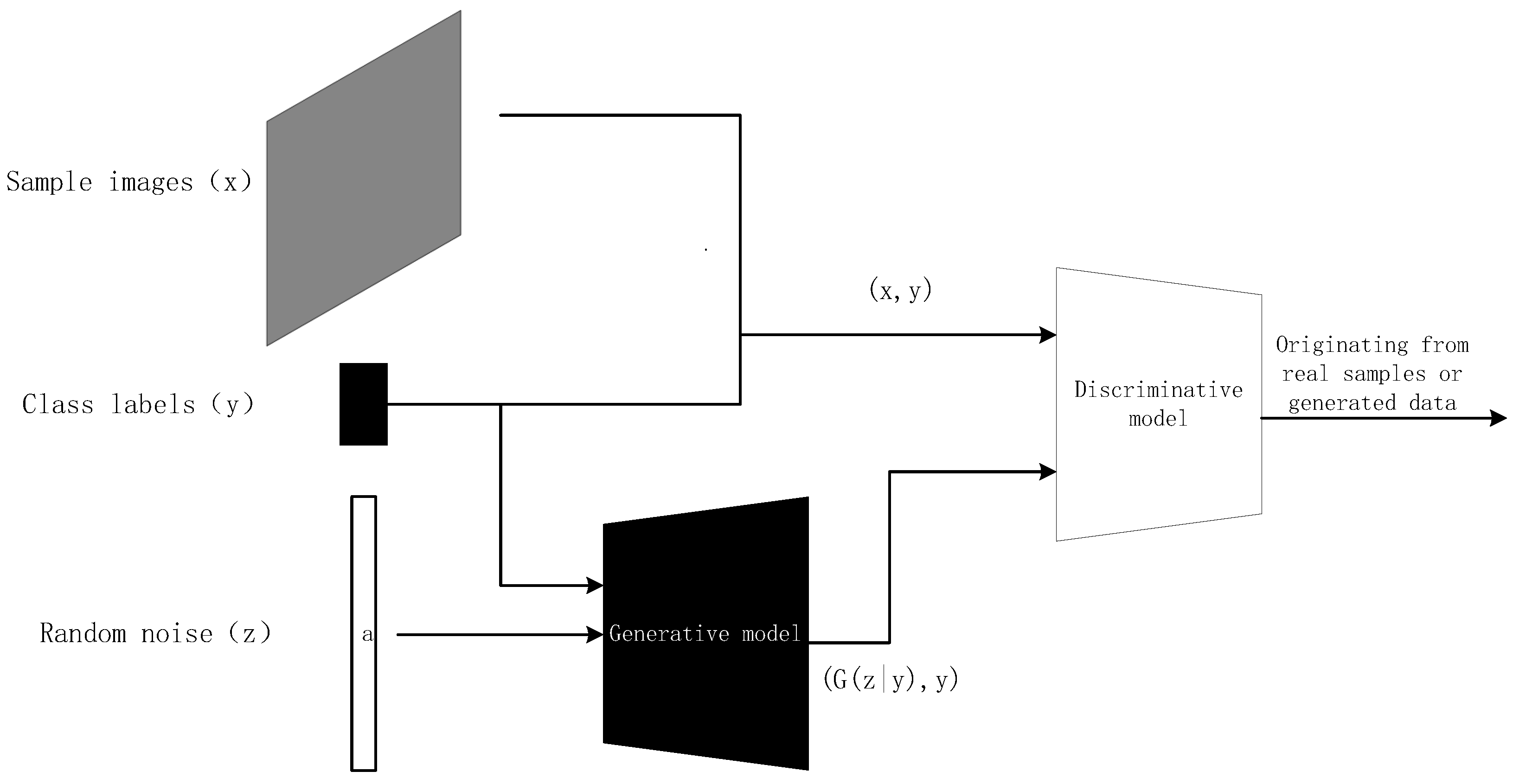
2.1. Generative Adversarial Networks

2.1.1. The Theory of Generative Adversarial Networks (GANs)

The generation method based on GANs avoids the probabilistic computational challenges posed by traditional models such as Markov chains and maximum likelihood estimation. Through adversarial training between the generator and discriminator, end-to-end backpropagation is achieved, effectively reducing the training difficulty of the generative model and improving training efficiency through the updating of network parameters. Additionally, GANs’ powerful representational capabilities support arithmetic operations in the latent vector space, converting them into corresponding operations in the feature space to learn the intrinsic representation of data. For example, given the attribute feature of an image in the latent space as a female wearing a gray T-shirt, by subtracting the feature vector of this female and adding the feature vector of another male, the network outputs an image of a male wearing a gray T-shirt. In real life, unlabeled data far exceed labeled data, and GANs excel at unsupervised learning from such unlabeled data, making full use of the vast resources available on the network. Although the data generated by GANs are synthetic, the model can generate data that are non-existent in real life but comparable in quality to real data. Therefore, GANs can learn to generate page layouts that do not exist but can rival real-world layouts by learning from existing page layouts.

2.1.2. The Principle of Generative Adversarial Networks (GANs)

Generative models can be broadly categorized into two types: those that represent the exact distribution function of the data and those that involve a fuzzy distribution function for generating new data. The GAN belongs to the latter category. The GAN, an unsupervised learning model, consists of a discriminator and a generator and is employed for generating images, audio, video, or text. Both the discriminator and the generator can be constructed using any neural network architecture, such as Artificial Neural Networks (ANNs), Convolutional Neural Networks (CNNs), Recurrent Neural Networks (RNNs), Long Short-Term Memory Networks (LSTMs), etc. GAN directly models the probability distribution of data samples implicitly through neural networks. The generator takes a random vector from a distribution, often a normal or uniform distribution denoted as $P\left(z\right)$, and transforms it into synthetic data $G\left(z\right)$.

The discriminator essentially functions as a binary classifier. Given a real image x, it outputs the probability that the input data are real by comparing them with the data generated by the generator, $G\left(z\right)$, where 0 represents fake and 1 represents true. The training process of GANs, as illustrated in Figure 1, involves the generator learning to produce a distribution similar to the real data distribution, while the discriminator learns to differentiate between inputs. The generator and discriminator engage in continuous adversarial training until the model reaches Nash equilibrium. At this equilibrium, the generator produces data that closely resemble the target distribution, and the discriminator cannot distinguish between real and generated data, assigning both probabilities of 1/2. In other words, the discriminator is unable to discern the difference between real and generated images, and both the generator and discriminator achieve optimal performance.

The training process of GANs involves a minimax game between the generator G and the discriminator D. The generator G takes a random vector z from a simple distribution $P_z$ and generates synthetic data $G\left(z\right)$. The discriminator D evaluates the probability that the input data are real. The objective function is defined as:

$${\min }_{G}m{ax}_D\left\{V(D,G)=E_{x-P_{data}}\left[\log D\left(x\right)\right]+E_{z-P_z}\left[\log (1-D\left(G\left(z\right)\right))\right]\right\}.$$

(1)

Here, $P_{data}$ represents the distribution of real data, and z is the input random vector to the generator. The first term represents the expected log probability that the discriminator correctly identifies real data, and the second term represents the expected log probability that the discriminator correctly identifies generated data as fake. The generator aims to minimize this objective function, while the discriminator aims to maximize it.

KS (KL divergence), also known as Kullback–Leibler divergence, is a critical concept in statistics used to measure the proximity between two probability distributions. The larger the KS divergence, the greater the difference between the probability distributions; conversely, smaller KS divergence indicates closer proximity between distributions. In GAN, KS divergence is effective in determining whether the generator and discriminator have reached Nash equilibrium. Assuming two continuous distributions P and Q, their KL divergence is defined as follows:

$$D_{KZ}\left(P\right|\left|Q\right)={\int }_{-\infty }^{+\infty }P\left(x\right)\log {\displaystyle \frac{P\left(x\right)}{Q\left(x\right)}}d\left(x\right).$$

(2)

The objective of the generator is to minimize the gap between the distribution $P_{data}\left(x\right)$ and the distribution $P_G(x; \theta )$ generated by feeding the random vector z into the generator, eventually approaching the same distribution. The generation principle is illustrated in Figure 2. Here, $\theta$ is determined by the network parameters, and the ultimate task of the network is to find $\theta$ to make $P_{data}\left(x\right)$ close to $P_G(x; \theta )$. The optimal generator achieved by the generative model is denoted as G*:

$$G*=\underset{G}{\min }\underset{D}{\max }V(D,G).$$

(3)

Given the data and a fixed generator G, consider $P_{data}\left(x\right)$ and $P_G\left(x\right)$ as constants. Adjust the discriminator D to maximize $V\left(D\right)$:

$$\mathrm{D}*\left(x\right)={\displaystyle \frac{P_{\mathrm{d}ata}\left(x\right)}{P_{\mathrm{d}ata}\left(x\right)+P_{\mathrm{G}}\left(x\right)}}.$$

(4)

Substituting D* into the previously optimal generation result, we obtain:

$$\underset{\mathrm{D}}{\max }\mathrm{V}(\mathrm{D},\mathrm{G})=-2\log 2+KL\left({\mathrm{P}}_{\mathrm{dan}}\left(x\right)\parallel {\displaystyle \frac{{\mathrm{P}}_{\mathrm{dan}}\left(x\right)+{\mathrm{P}}_{\mathrm{G}}\left(x\right)}{2}}\right)+KL\left({\mathrm{P}}_{\mathrm{G}}\left(x\right)\parallel {\displaystyle \frac{{\mathrm{P}}_{\mathrm{dan}}\left(x\right)+{\mathrm{P}}_{\mathrm{G}}\left(x\right)}{2}}\right).$$

(5)

We adjust D to maximize the value of $\mathrm{V}(\mathrm{G}, \mathrm{D})$, where the two KL divergences together constitute the maximum, thus measuring the degree of difference between $P_{data}\left(x\right)$ and $P_G\left(x\right)$. The generator G aims to minimize the KL divergence between the generated data and real data, while the discriminator D attempts to maximize it. The model training process is illustrated in Figure 3, where the horizontal line z represents the input random vector, the horizontal line x represents real data, and the arrows between the two parallel lines represent the mapping from the input random vector to the generated data, i.e., the mapping from uniformly distributed data to non-uniformly distributed data. The green solid line reflects the distribution of generated data, the black dashed line reflects the distribution of real data, and the blue dashed line represents the discriminator. The model training process is illustrated in Figure 3, where the horizontal line z represents the input random vector, the horizontal line x represents real data, and the arrows between the two parallel lines represent the mapping from the input random vector to the generated data, i.e., the mapping from uniformly distributed data to non-uniformly distributed data. The green solid line reflects the distribution of generated data, the black dashed line reflects the distribution of real data, and the blue dashed line represents the discriminator. Figure 3a–d represent the model training initial state, fixing G to train D, fixing D to train G, and the final convergence stage, respectively. By the (d) stage of training, the distribution of generated data perfectly matches the distribution of real data.

The training algorithm for GAN discriminators and generators, as shown in Algorithm 1, involves sampling m examples $\{x_1,\dots ,x_m\}$ from the real data distribution Pdata and m examples $\{z_1,\dots ,z_m\}$ from the generated data distribution $P_G$ to enhance training efficiency. During the training process, the discriminator D undergoes cyclic training with real and generated data distributions for k iterations, followed by training the generator G with a smaller learning rate. G progressively reduces the gap between real and generated samples during iterative training, achieving convergence.

Algorithm 1 GAN Training Algorithm

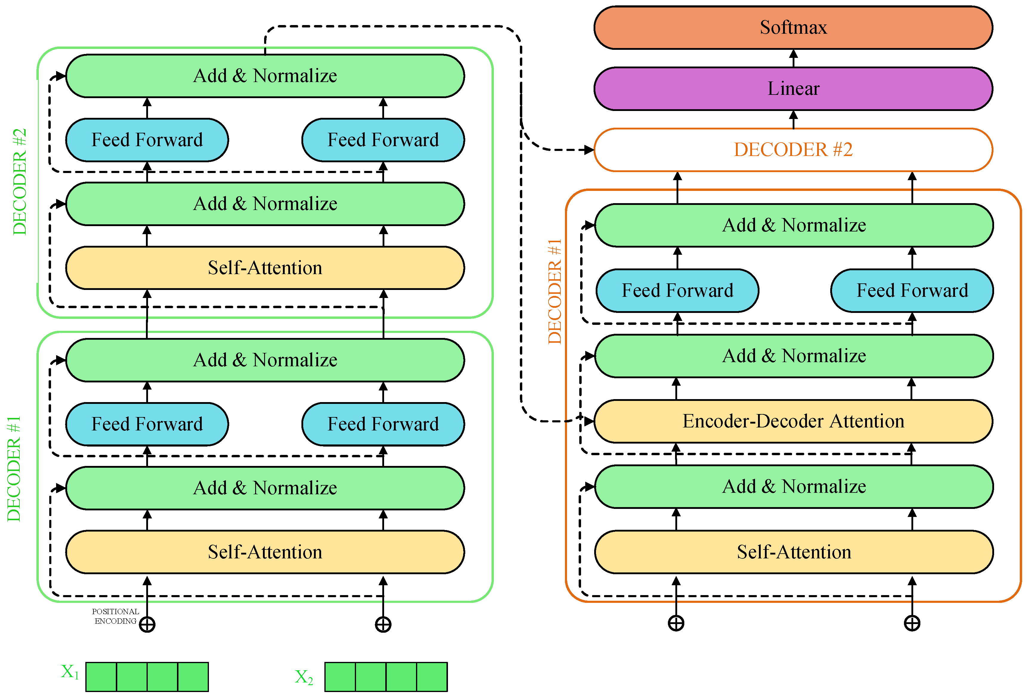
1: for number of training iterations do 2:   for k steps do 3:      Sample m sets of noise data $\{z_1,\dots ,z_m\}$ from the random distribution $P_G\left(z\right)$; 4:      Sample m sets of samples x1,…, xm from the real data distribution $P_{data}\left(x\right)$; 5:      Update the D network: ${\nabla }_{\theta d}{\displaystyle \frac{1}{m}}{\sum }_{i=1}^m[\log D(x^{\left(i\right)}+\log (1-D\left(G\left(z^{\left(i\right)}\right)\right))]$; 6:   end for 7:   Sample m sets of noise data $\{z_1,\dots ,z_m\}$ from the random distribution $P_G\left(z\right)$; 8:   Update the G network: ${\nabla }_{{\theta }_g}{\displaystyle \frac{1}{m}}{\sum }_{i=1}^m \log (1-D\left(G\left(z^{\left(i\right)}\right)\right))$. 9: end for

2.2. Transformer

The Transformer consists of an encoder and a decoder. The encoder maps the input sequence $x=(x_1,\dots ,x_n)$ to a continuous sequence $z=(z_1,\dots ,z_n)$. The decoder generates a sequence $y=(y_1,\dots ,y_m)$ step by step based on the given values of z. The stacked encoder and decoder component structure is illustrated in Figure 4, where the left side represents the encoder component and the right side represents the decoder component. Each encoder has the same structure, consisting of two sub-layers with different weights. The input passes through a self-attention layer and then is fed to a feed-forward neural network layer. In addition to these two sub-layers, the decoder also includes an encoder–decoder attention layer, similar to Seq2Seq, which helps the decoder focus on relevant parts of the input data. Between these layers, connections are made through Add and Normalize, involving mainly residual connections and normalization operations. Add and Normalize breaks the symmetry of the neural network, improving the issue of network degradation. It accelerates model convergence by optimizing the normalization process and addresses the problem of gradient vanishing in deep learning.

By treating data as a sequence, the Transformer initially processes the input data through embedding to obtain vector representations. Subsequently, position encoding is applied to the corresponding data in the sequence to prevent data misalignment. Through a self-attention mechanism, the data are mapped to triplets Q (Query), K (Key), and V (Value) for representation, and vectors are output. The formula for the self-attention mechanism is as follows:

$$\mathrm{Attention}(Q,K,V)=\mathrm{softmax}\left({\displaystyle \frac{Q{K}^T}{\sqrt{d_k}}}\right)V.$$

(6)

In the above equation, Q represents the query matrix, and K represents the key matrix, both of which use dot product matching. The result is the attention matrix, which effectively reflects the semantic relevance between Q and K. Additionally, $d_k$ in the equation denotes the channel dimension, and the weights obtained by applying the Softmax function to the calculated values are further used to obtain the values of self-attention.

In each layer of the Transformer encoder and decoder structure, in addition to the multi-head self-attention mechanism, there is also a fully connected feed-forward network. The fully connected feed-forward network consists of two linear transformations followed by a ReLU activation function. The computational formula is as follows:

$$\mathrm{FFN}\left(x\right)=\max (0,x{W}_1+b_1)W_2+b_2.$$

(7)

Although the linear transformations at different positions between layers in the fully connected feed-forward network are the same, the network parameters used within them are different. The purpose of positional encoding is to obtain accurate information about the positions of input sequences, thus compensating for the lack of positional information in Transformer models compared to recursive networks and convolutional neural networks. By adding positional encoding to the bottom input of the encoder and decoder, the bottom input and positional encoding have the same dimensions for addition, achieving an accurate description of the relative and absolute positions of input sequence data. There are various methods for performing positional encoding, and the Transformer model uses cosine and sine functions with different frequencies.

$$P{E}_{(pos,2i)}=sin\left(pos/{10000}^{2i/d_{modd}}\right),$$

(8)

$$P{E}_{(pos,2i+1)}=cos\left(pos/{10000}^{2i/d_{model}}\right),$$

(9)

where i represents the dimension and $pos$ represents the position, indicating that each dimension of the positional encoding corresponds to a sine function.

2.3. TGAN

2.3.1. TGAN Principle

The starting point for the TGAN generator is no longer just an unknown noise distribution but rather labels or more detailed features of images, enabling the synthesis of forged samples. During the training of the TGAN model, the generator learns to produce realistic samples that match the labels of the dataset, while the discriminator learns to distinguish between fake samples and label pairs from the generator and real samples and label pairs from the training set. By introducing conditional variables into both the generator and discriminator, forming combined conditional variables $\mathrm{D}(\mathrm{x}, \mathrm{y})$ and $\mathrm{G}(\mathrm{z}, \mathrm{y})$, the objective function of the TGAN becomes:

$$\underset{G}{\min }\underset{D}{\max }V(D,G)={\mathbb{E}}_{\mathbf{x}\sim p_{\mathrm{dan}}\left(\mathbf{x}\right)}\left[\log D\left(\mathbf{x}\right|\mathbf{y})\right]+{\mathbb{E}}_{\mathbf{z}\sim p_z\left(\mathbf{z}\right)}\left[\log (1-D\left(G\left(\mathbf{z}\right|\mathbf{y})\right))\right].$$

(10)

The TGAN model architecture is illustrated in Figure 5. From the figure, it can be observed that class labels (y) are input into the generative model along with random noise (z) and into the discriminative model along with sample images (x). Additionally, the discriminative model also receives input from the generated samples by the generative model ($\mathrm{G}(z\mid \mathrm{y})$).

2.3.2. Generator

The generator model with the added Transformer module is illustrated in Figure 6. The generator has two inputs: a 100-dimensional vector randomly sampled from the latent space (left) and a class label y (right). The model employs a neural network structure consisting of 2 layers of deconvolution and 1 layer of convolution. Initially, a 100-dimensional random vector is input into the generator and transformed into a 320-dimensional vector through a fully connected layer. The role of the fully connected layer is to fuse image features and obtain advanced meanings of these features, achieved through multiple pooling layers and convolutional layers. The vector is then reshaped through a reshape layer, altering its shape through matrix transformation, and the output is sent to the transformer_block layer for feature extraction. The data processed by the Transformer module are flattened using the flatten layer, turning the vector one-dimensional. The network layers handling the Transformer module include the mentioned dense layer, reshape layer, transformer_block layer, and flatten layer. These layers primarily aim to extract more refined features from the image, thereby enhancing the accuracy of image generation and ensuring faster convergence of the model.

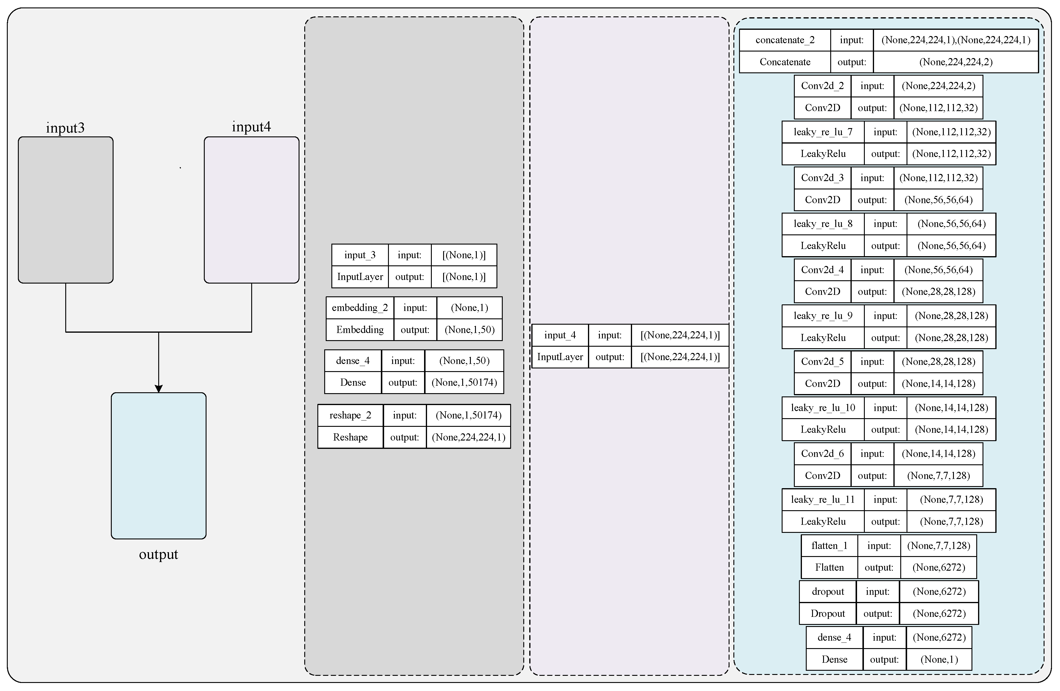
2.3.3. Discriminator

The discriminator takes a grayscale image with pixel size 224 × 224 as input and outputs a binary prediction indicating whether the image is real (class = 1) or fake (class = 0). An output of 1 indicates that the discriminator considers the generated image to be close to a real image, while an output of 0 signifies that the discriminator deems the generated image quality to be poor. The discriminator model is designed as a moderate convolutional neural network, using the LeakyReLU activation function with a slope of 0.2 and employing 2 × 2 strides for downsampling. As shown in Figure 7, the model has two inputs: on the left, the input is the class label (y) and an embedding layer of size 50. This input uses integers as class labels, achieving the effect of conditioning on the input image with respect to its class. On the right, the input is an image defined by the CGAN discriminator model, with a size of 224 × 224. The class label is passed through an embedding layer with a size of 50, where each class is mapped to a different 50-dimensional vector representation, learned by the discriminator. The embedded output is then passed through a fully connected layer with linear activation, reshaped into an activation map of size 224 × 224, and concatenated with the input image. This operation achieves a dual-channel input image effect when passed to the next convolutional layer. The update of the discriminator is implemented using the define_discriminator() function, where the parameterized shape of the input image is used after the embedding layer to define the activation of the fully connected layer for reshaping its output. Finally, the discriminator is defined, compiled, and returned, with the number of classes also parameterized in the function and set.

2.4. Integrated Layout Optimization

To directly optimize layout quality during training, we integrate the energy-based evaluation metrics into the generator’s objective function. The total loss consists of two components:

$${\mathcal{L}}_{total}={\mathcal{L}}_{adv}+\lambda \sum _{i=1}^6{\omega }_i{E}_i\left(X\right)$$

(11)

where the following are true:

• ${\mathcal{L}}_{adv}$ is the standard adversarial loss from Equation (1).
• $\lambda$ is a balancing coefficient (set to 0.8 through grid search).
• $E_i\left(X\right)$ denotes the six energy terms defined in Section 3.4.2.
• ${\omega }_i$ are adaptive weights updated every 5 epochs based on validation performance.

This formulation follows recent work on physics-informed neural networks [22], where domain-specific constraints are directly embedded into the learning objective. As shown in Algorithm 2, during each training iteration, we have the following:

Algorithm 2 Integrated Training Process.

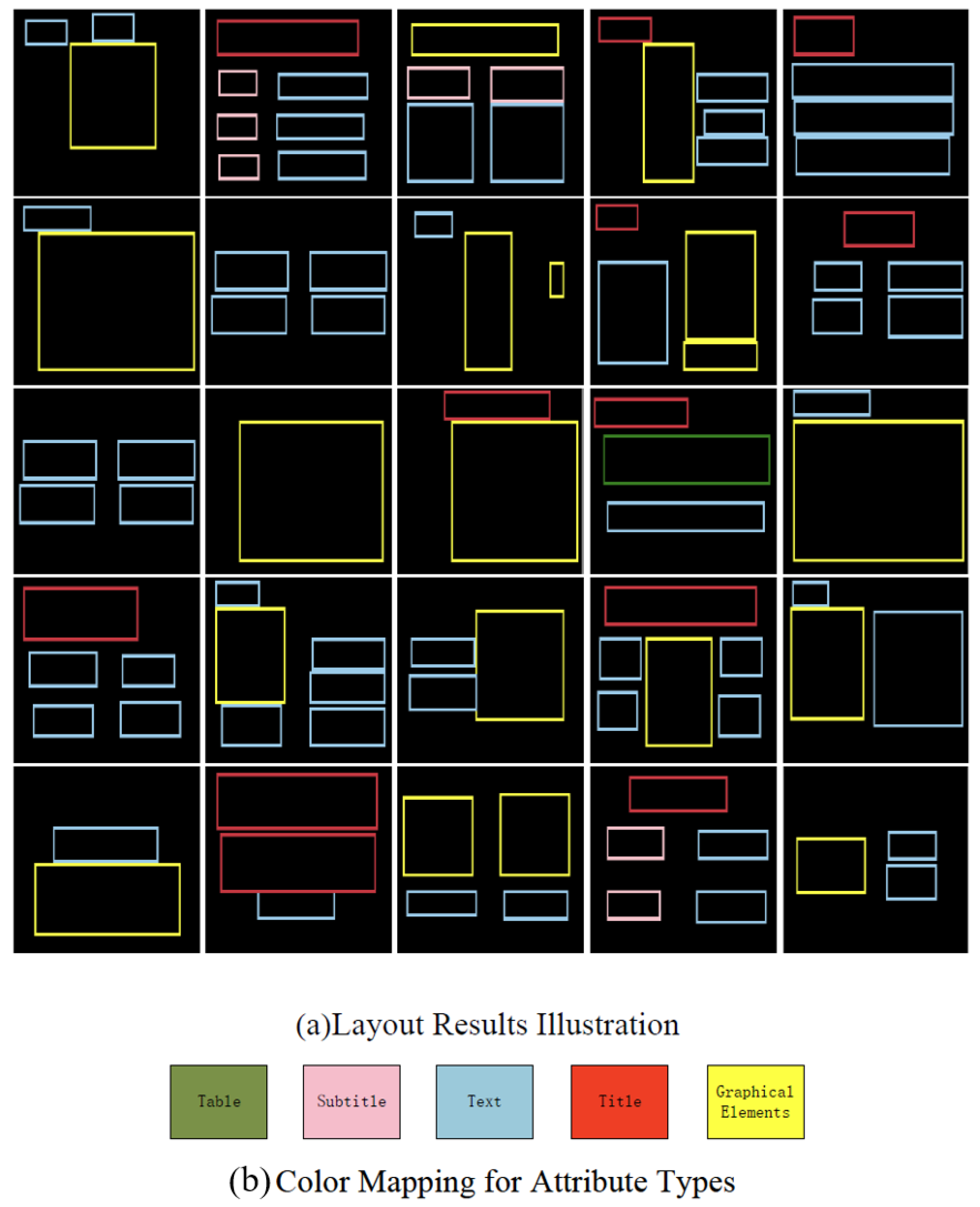
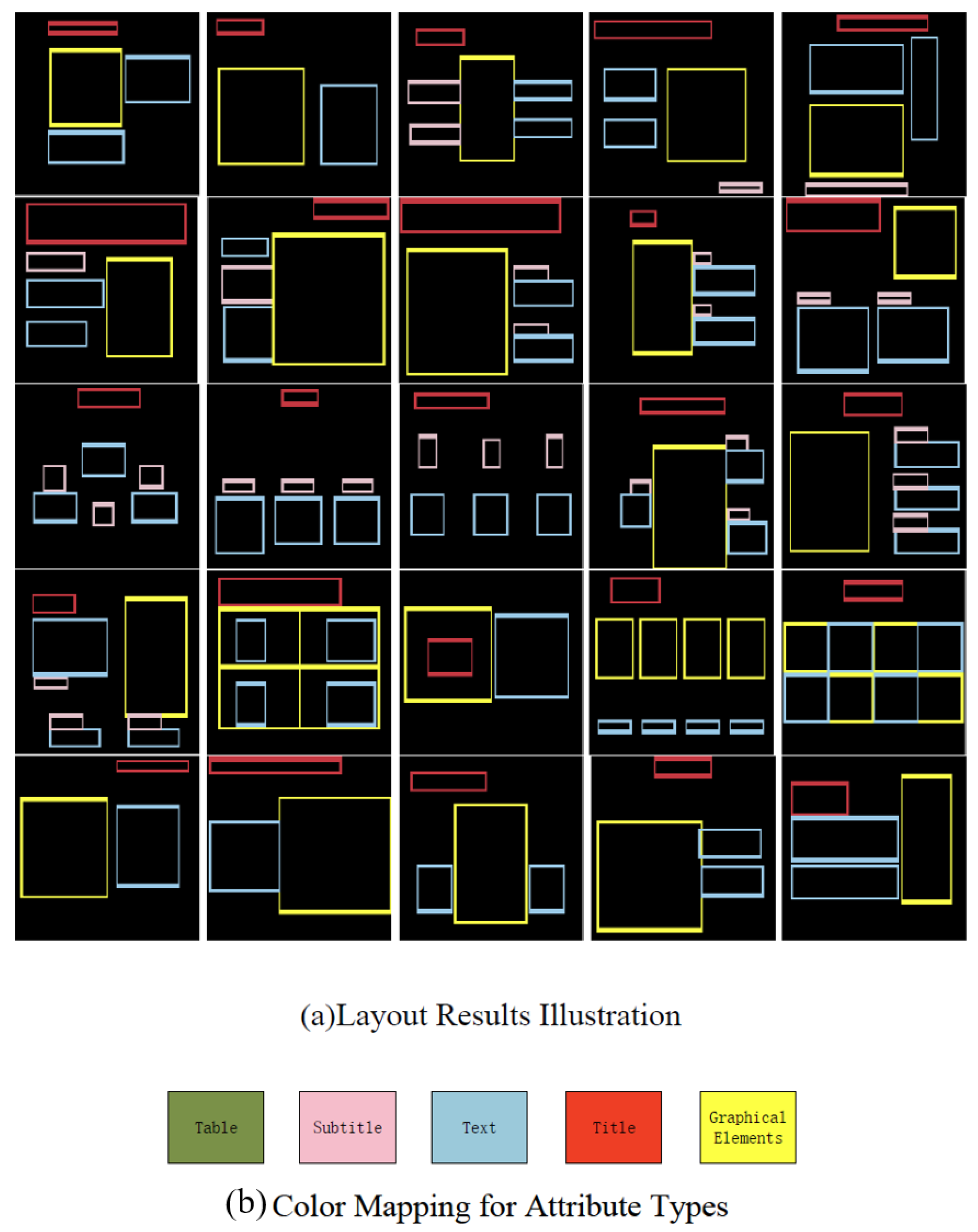
1: Sample noise $z\sim p_z$, real data $x\sim p_{data}$ 2: Generate layouts $G\left(z\right|y)$ 3: Compute adversarial loss ${\mathcal{L}}_{adv}$ via Equation (1) 4: Calculate layout energy terms $\{E_1,\dots ,E_6\}$ 5: Update generator parameters: ${\theta }_G\leftarrow {\theta }_G-\eta \nabla ({\mathcal{L}}_{adv}+\lambda \sum {\omega }_i{E}_i)$ 6: Update discriminator normally via Equation (1)

The adaptive weighting mechanism automatically adjusts ${\omega }_i$ based on the relative difficulty of satisfying each constraint. For example, if alignment ($E_{align}$) has higher validation error than other terms, its weight ${\omega }_{align}$ increases by 15% for the next 5 epochs. This ensures balanced optimization across all quality dimensions.

3. Experiment

3.1. Dataset

The content types included in page layouts are diverse, mainly comprising titles, subtitles, tables, graphics, text, and more. Additionally, the real sizes of different page layouts vary, making it challenging to treat different page layout samples as input data for object information. Therefore, this paper addresses different page layouts through the following two approaches:

• To address the issue of varying real sizes across all page layouts, all real data were standardized to a size of 224 × 224 pixels.
• Elements within page layouts, such as titles, subtitles, tables, graphics, and text, were abstracted into differently colored boxes to disregard internal content, text, images, formats, and other factors that could influence the model’s overall page layout generation.

For example, as illustrated in Figure 8, the page layout Figure 8a was standardized to a size of 224 × 224 pixels, and the elements within the page were marked with different colors. The final result is shown in Figure 8b.

The overall dataset consists of 7256 training samples, with 5804 training samples, accounting for 80% of the entire dataset, and 1452 testing samples, representing 20% of the entire dataset. To visually distinguish semantic elements within the page layout, the labeling process uses green to represent tables, red for titles, pink for subtitles, blue for text, and yellow for graphics. Through a statistical analysis of the frequency of appearance of various semantic elements in the dataset, graphics and text account for 99.3% and 89.9%, respectively, indicating that most page layouts include graphics and text. Titles and subtitles account for 78.5% and 56.4%, respectively, while tables make up 42.8%. This suggests that in page layouts, graphics and text are essential elements, followed by titles, subtitles, and tables in terms of importance.

3.2. Data Augmentation and Pre-Training

To address the limited dataset size (7256 samples), we implemented the following strategies to improve model robustness:

• Geometric Augmentation: random scaling (0.8–1.2×), rotation (±15°), and translation (±10% of layout width/height) to simulate diverse design scenarios.
• Element-wise Augmentation: random permutation of element types (e.g., swapping text and image positions) and perturbation of bounding box coordinates (±5 pixels).
• Pre-training: the Transformer module was pre-trained on the RICO dataset [38] (72k mobile UI layouts) to learn general layout patterns, followed by fine-tuning on our domain-specific data.

These techniques increased the effective training data diversity, while pre-training reduced convergence time by 40% compared to training from scratch.

3.3. Experimental Considerations Detail

The experimental implementation employed Python version 3.9, the PyTorch 2.3.0 framework, and CUDA version 12.2.19. The graphics card used was the NVIDIA GeForce RTX 3060 8G. During the training process, the model’s learning rate was set to 0.0001, and the batch size was set to 64. The optimizer used was Adam, with $\epsilon ={10}^{-7}$, $\beta 1=0.5$, and $\beta 2=0.9$. To ensure sufficient training of the generator, discriminator, and encoder, and to avoid the discriminator suppressing the learning of the generator and encoder due to a too-fast learning rate, the training iterations for the generator and encoder were increased in the experiment to enhance their learning capabilities.

The revised TGAN objective combines adversarial loss with layout energy terms:

$${\mathcal{L}}_{total}=\underset{\mathrm{Adversarial} \mathrm{loss}}{\underbrace{\mathbb{E}\left[\log D\right(x\left|y\right)]+\mathbb{E}[\log (1-D(G\left(z\right|y\left)\right)\left)\right]}}+\lambda \sum _{i=1}^6{\omega }_i{E}_i\left(X\right)$$

(12)

where $\lambda$ controls the weight of layout quality metrics (alignment, balance, whitespace, etc.) derived from our energy model.

3.4. Evaluating Indicator

3.4.1. Subjective Scoring

This paper conducts user ratings on the layouts of presentation samples, with scores ranging from 0 to 10, where higher scores indicate better layout quality. In practice, users primarily judge the layout of the presentation visually and subjectively. Combining aesthetic principles and layout-related criteria, and without considering the overall coordination of background and color, users subjectively evaluate the layout quality of samples based on the following two aspects:

• Rationality of object placement: Whether the object positions look aesthetically pleasing, whether objects are aligned with each other, and whether objects are within safe locations on the page. Aligning objects enhances the visual understanding of their relationship for readers and contributes to the overall aesthetic and orderly appearance of the layout.
• Readability of text: whether there is overlap between text and images that affects readability.

3.4.2. Objective Scoring

For the objective evaluation of layout quality, it is primarily based on aesthetic principles and layout-related criteria. This paper employs an energy-based model $E(X;\theta )$, using parameter $\theta$ to assess the layout X of the presentation. The overall quality of the layout is measured by the weighted sum of energy terms:

$$E(X;\theta )=\sum _i{\omega }_i{E}_i(X;{\alpha }_i).$$

(13)

In this context, the design layout X is defined for each object’s position, metadata, width, and height, with $theta$ representing the model parameters. The model parameters are divided into two groups, $\theta =[\omega ; \alpha ]$. Each energy term $E_i$ has positive weights $omeg{a}_i$, and most terms involve non-linear parameters $alph{a}_i$. The energy function incorporates various design principles, including alignment, balance, white space, scale, overlap, and boundaries. The definitions of each energy term are provided below.

• Alignment
  Alignment is crucial for design, especially in limited space where efficient information transmission and aesthetically pleasing organization are prioritized. The first consideration in this context is the alignment of various elements. This paper defines six possible alignment types: Left, X-center, Right, Top, Y-center, and Bottom. Before defining the alignment energy term, an analysis phase is executed, marking all aligned objects and alignment groups.
  A simple heuristic algorithm is employed to compute the alignment of object bounding boxes. Initially, the difference between the edges or center positions of the bounding boxes must be smaller than a threshold:

  $$A_{ij}^a=\left(\begin{array}{c}{d}_{ij}^a<{\tau }_{align}\end{array}\right),$$

  (14)

  where a is the alignment type and $d_{ij}^a$ represents the distance between two objects i and j, depending on the alignment type used for the bounding boxes of the objects. For example, if a = Left, then $d_{ij}$ Left measures the difference between the left edges of the bounding boxes of two objects. The threshold is set to ${\tau }_{align}$ =0.065, allowing slightly misaligned objects to still be marked as aligned. Secondly, if an object is positioned between other objects, the objects may not align:

  $$B_{ij}=(b_{ij}<1),$$

  (15)

  where $b_{ij}$ is the number of objects between i and j. Next, the alignment indicator is defined. The alignment indicator variable between objects i and j, denoted as $I_{ij}^a$, is a combination of the terms mentioned above:

  $$I_{ij}^a=A_{ij}^a\wedge B_{ij}\wedge N_i^a\wedge N_j^a.$$

  (16)
  In each axis, two objects typically align with only a single type. The minimum alignment distance $d_{ij}^a$ is set to 1, while the other two are set to 0. However, if all types are perfectly aligned ($d_{ij}^a$= 0 for all types), then all three indicators are set to 1.
  Next, the aligned group is defined as a set of connected aligned objects. If objects i and k are aligned and objects k and j are aligned with the same type, then i and j are set to be aligned, i.e., $I_{ij}^a=I_{ik}^a\wedge I_{kj}^a$.
  Finally, the alignment energy term is defined, measuring the proportion of objects aligned with a specific alignment type. Larger alignment groups are encouraged, as they result in simpler designs and greater uniformity between objects. The alignment energy term measures the score of pairs of objects aligned with type a:

  $$E_{align}^a=S\left(\left|{\displaystyle \frac{1}{n^2}}\sum _{i\in \left(all\right)}\left(N_i^a+\sum _{j\in \left(all\right)}{I}_{ij}^a\right)-1\right|;{\alpha }_a\right),$$

  (17)

  where n is the number of objects and $I_{ij}^a$ indicates whether objects i and j are aligned according to type a. Different alignment types define separate energy terms. $N_i^a$ indicates whether i is a text object aligned internally within type a. Each feature is transformed by $S(x;\alpha )$, which is a smooth step function defined by the following formula. The parameter $\alpha$ controls the smoothness of the step, with larger $\alpha$ values making the energy more sensitive to smaller changes.

  $$S(x;\alpha )={\displaystyle \frac{arctan\left(x\alpha \right)}{arctan\left(\alpha \right)}}.$$

  (18)
• Balance
  The term “balance” refers to the equal distribution of weight on a page, indicating symmetry or asymmetry in terms of color, size, shape, and texture. This paper primarily focuses on the symmetry of object sizes on the page. The overall balance is measured using a binary mapping (along the axis flip) of text or graphic objects. For x-axis symmetry, the balance energy term is defined as:

  $$S_{x-symm}=\sum _{c\in (graphic,text)}\left|{\displaystyle \frac{{\sum }_p{I}_{flip(p,x,G)}^c{I}_p^c}{{\sum }_p{I}_p^c}}-1\right|,$$

  (19)

  $$E_{x-symm}=S\left(S_{x-symm};{\alpha }_{txs}\right),$$

  (20)

  where $I_p^c$ represents a binary variable indicating whether pixel p belongs to the class $c\in (graphic, text)$ and $flip(p,x,G)$ denotes the symmetric counterpart of pixel p along the x-axis in the image G. A similar balance energy term $E_{y-symm}$ is defined for y-axis symmetry, where $flip(p,x,G)$ represents the y-axis symmetric term.
• White space
  In graphic design, white space is the foundation of readability and aesthetics. The distance between objects is closely related to their correlation; the closer the objects are, the more likely they are to be associated with each other. White space also influences the overall design style, and many modern designs incorporate significant empty spaces. However, excessive white space between objects can distract the reader’s attention. The blank space should ideally constitute around half of the total page area. The energy term for white space is defined as follows:

  $$E_{whiteSpace}=S\left(\left|4{\left({\displaystyle \frac{{\sum }_p{I}_p^o}{wh}}-{\displaystyle \frac{1}{2}}\right)}^2\right|;{\alpha }_{ws}\right),$$

  (21)

  where $I_p^0$ is a binary variable indicating whether the pixel p is covered by an object and w and h are the width and height of the entire page, respectively.
• Scale
  The scale of an object determines its usability and style. Objects must be large enough for visibility but not too large, as it can lead to a cluttered and unattractive design. Objects in the layout can be broadly categorized into text and graphics. The size of text objects is defined as follows:

  $$M_i^s=\left|{\displaystyle \frac{{\tau }_s{M}_i^h}{F_i^{l}h}}-{\displaystyle \frac{1}{20}}\right|,$$

  (22)

  where $M_i^h$ represents the height of the text object, $F_i^l$ represents the number of lines in the text object, ${\tau }_s$ is the scaling parameter, and normalization is performed with respect to the page height h. In this paper, ${\tau }_s$ = 1 is used uniformly. Using smaller values, such as ${\tau }_s$ = 0.4, will increase the size of text objects. The size of graphic objects is defined as follows:

  $$M_i^s=\left|{\displaystyle \frac{M_w^i{M}_h^i}{wh}}-{\displaystyle \frac{1}{4}}\right|,$$

  (23)

  where $M_w^i$ and $M_h^i$ represent the width and height of the bounding box of the graphic object and w and h are the width and height of the page. The scale energy term for text objects is defined as:

  $$E_{textsize}={\displaystyle \frac{1}{n_t}}\sum _{i\in \left(text\right)}S(M_i^s;{\alpha }_{ts}),$$

  (24)

  where $n_t$ is the number of text objects. The scale energy term EgraphicSize for graphic objects is defined similarly to EtextSize.
• Overlap
  Overlap between objects is common in many designs, but some overlaps can impact information retrieval. Three types of overlaps are defined, including overlap between text objects, overlap between graphic and text objects, and overlap between graphic objects. Separate energy terms are defined for each overlap type and summed over overlapping pixels p. The overlap energy term between text objects is defined as:

  $$o_{textTextOverlap}={\displaystyle \frac{{\sum }_p{A}_p^t}{wh}},$$

  (25)

  $$E_{textTextOverlap}=S\left(o_{textTextOverlap};{\alpha }_{to}\right),$$

  (26)

  where $A_p^t$ represents the pixels overlapped between text objects. EgraphicTextOverlap and EgraphicGraphicOverlap are similarly defined for overlap between text and graphic objects and overlap between graphic objects, respectively.
• Boundary
  The ability to control the extension of objects beyond the boundaries is achieved by calculating the portion of objects that exceeds the boundaries. Two separate energy terms, namely, the graphic boundary energy term and the text boundary energy term, are defined for this purpose. The graphic boundary energy term is defined as follows:

  $$B_{graphic}={\displaystyle \frac{1}{n}}\sum _{i\in \left(graphic\right)}\left(1-{\displaystyle \frac{{\sum }_{p\in i}{A}_p{I}_p}{{\sum }_{p\in i}{A}_p}}\right),$$

  (27)

  $$E_{graphicBoundary}=S(B_{graphic};{\alpha }_{gb}),$$

  (28)

  where ${\sum }_{p\in i}{A}_p$ represents the sum of all pixels in object i and ${\sum }_{p\in i}{A}_p{I}_p$ represents the sum of pixels in object i that are within the page boundaries. The definition of the text boundary energy term $EtextBoundary$ is similar to that of the graphic boundary energy term. By defining energy terms for alignment, balance, white space, scale, overlap, and boundary separately, it is possible to provide an objective evaluation of the presentation layout based on its detailed aspects. The range of values for each energy term is [0,1]. All energy terms are weighted equally with $omega$ = 1/6, measuring the overall quality of the layout. The closer the weighted sum of energy terms is to 0, the better the layout quality.

3.5. Training Process

3.5.1. Data Preparation

The dataset consists of 7256 page layouts, each standardized to a size of 224 × 224 pixels. Elements within the layouts (e.g., titles, subtitles, tables, graphics, and text) are abstracted into colored boxes, with colors mapped to specific element types (e.g., green for tables, red for titles). The dataset is split into training (80%), validation (10%), and test (10%) sets, ensuring a balanced distribution of element types across subsets.

3.5.2. Hyperparameter Tuning

We employ the Adam optimizer with an initial learning rate of 0.0001, ${\beta }_1=0.5$, and ${\beta }_2=0.9$. The batch size is set to 64, and the model is trained for 100 epochs with early stopping if the validation loss does not improve for 10 consecutive epochs. Hyperparameters are tuned using grid search, with the best combination selected based on validation set performance.

3.5.3. Model Training and Optimization

The generator and discriminator are trained alternately, with the discriminator updated $k=5$ times for each generator update. To prevent overfitting, we apply dropout (rate = 0.3) and weight decay (L2 regularization with $\lambda =0.01$). The training process is monitored using validation set metrics, including alignment, overlap, and balance scores.

3.5.4. Model Evaluation Strategies

Model performance is evaluated using both subjective and objective metrics. Subjective scores are obtained from 10 human evaluators, while objective scores are computed using the energy-based model described in Section 3.4.2. Additionally, we visualize training curves (e.g., generator and discriminator losses) and generated layouts at different training stages to assess model convergence and sample diversity.

3.6. Ablation Experiment Result Analysis

To validate the impact of individual components in TGANs, we conduct controlled experiments with five configurations:

• Standard GAN: basic GAN without Transformer or conditioning.
• TGAN w/o Self-Attention: remove self-attention modules.
• TGAN w/o Conditioning: remove conditional inputs (labels).
• Fixed-Weight: TGAN with fixed ${\omega }_i$ weights.
• Adaptive-Weight (Full): Our complete model with dynamic ${\omega }_i$.

The ablation study results (Table 1) reveal the following key insights:

• Self-attention impact: Removing self-attention (TGAN w/o SA) degrades alignment by 23.6% (0.89→0.68) and increases overlap by 257% (0.07→0.25), confirming its critical role in modeling spatial dependencies.
• Conditioning necessity: disabling conditional inputs (TGAN w/o Cond) reduces balance by 16.5% (0.85→0.71), indicating that label guidance stabilizes layout semantics.
• Adaptive-Weight superiority: Adaptive-Weight outperforms Fixed-Weight in all metrics (e.g., +8.5% alignment), demonstrating the necessity for dynamic constraint balancing.
• Standard GAN limitation: the basic GAN achieves the lowest scores, proving that vanilla architectures struggle with layout generation.

Table 1. Component-wise ablation study on layout quality metrics (bold represents the best result).

Method	Alignment	Overlap	Balance	White Space	Boundary	Scale
Standard GAN	0.62	0.31	0.58	0.61	0.72	0.65
TGAN w/o Self-Attention	0.68	0.25	0.63	0.66	0.78	0.70
TGAN w/o Conditioning	0.74	0.19	0.71	0.70	0.82	0.75
Fixed-Weight	0.82	0.12	0.78	0.75	0.87	0.81
Adaptive-Weight (Full)	0.89	0.07	0.85	0.82	0.93	0.88

Table 1. Component-wise ablation study on layout quality metrics (bold represents the best result).

Method	Alignment	Overlap	Balance	White Space	Boundary	Scale
Standard GAN	0.62	0.31	0.58	0.61	0.72	0.65
TGAN w/o Self-Attention	0.68	0.25	0.63	0.66	0.78	0.70
TGAN w/o Conditioning	0.74	0.19	0.71	0.70	0.82	0.75
Fixed-Weight	0.82	0.12	0.78	0.75	0.87	0.81
Adaptive-Weight (Full)	0.89	0.07	0.85	0.82	0.93	0.88

3.7. Comparison Experiment Result Analysis

We compare the TGAN and GAN in both generated page layout and subjective–objective scoring to highlight the performance of the TGAN. Firstly, we randomly selected 25 layouts from the results of the TGAN. The layout diagrams are shown in Figure 9a, and the correspondence between object types and colors is illustrated in Figure 9b.

Similarly, we randomly selected 25 layouts from the results generated by the GAN. The layout diagrams are presented in Figure 10a, and the correspondence between object types and colors is depicted in Figure 10b.

Compared to the results generated by the GAN, the TGAN exhibits a more aesthetically pleasing layout overall. In summary, the following points highlight the differences:

• Results generated by the TGAN exhibit better alignment and fewer instances of overlap, facilitating more efficient information conveyance.
• TGAN layouts adhere to topological constraints among objects, arranging elements with constraints in a logical manner on the page, making the relationships between elements clear and maximizing their expressive potential.

In order to better assess the subjective and objective scores of the TGAN, we selected 200, 400, and 600 generated samples from the TGAN, GAN, LayoutTransformer [6], VTN [7], L-CGAN [5], and PLAY [8], and we evaluated the results using subjective and objective assessment methods. The evaluation results are shown in

Table 2. Comparative evaluation of layout generation methods (bold represents the best result).

Method	Samples	Subjective Score		Objective Score
		Mean	Variance	Mean	Variance
GAN	200	7.992	0.503	0.078	0.0032
GAN	400	7.876	0.521	0.065	0.0035
GAN	600	8.105	0.417	0.053	0.0029
LayoutTransformer	200	7.983	0.497	0.076	0.0034
LayoutTransformer	600	8.173	0.421	0.057	0.0031
VTN	600	8.123	0.412	0.060	0.0032
L-CGAN	600	7.674	0.501	0.064	0.0031
PLAY	600	8.207	0.445	0.059	0.0030
TGAN (Ours)	200	8.45	0.38	0.048	0.0023
TGAN (Ours)	400	8.52	0.36	0.045	0.0020
TGAN (Ours)	600	8.60	0.35	0.042	0.0018

.

The results in Table 2 indicate that in subjective evaluation, under the three different sampling approaches, the mean layout scores of the TGAN are consistently higher than those of the other methods, while the variances are consistently lower. Notably, our TGAN demonstrates progressive quality improvement with more training samples, whereas baseline methods plateau after 400 samples. This suggests superior learning capability for complex layout patterns. In terms of objective evaluation, both the mean and variance of the energy item weighted sum for the TGAN are lower than those of the other methods. Overall, this suggests that the TGAN exhibits higher layout quality and stability compared to other methods.

3.8. Quantitative Metrics and User Study

3.8.1. Quantitative Evaluation of Generation Quality

To comprehensively evaluate the quality and diversity of generated layouts, we introduce two widely used metrics for generative models:

• Fréchet Inception Distance (FID): This measures the similarity between the distribution of generated samples and real data. A lower FID indicates better generation quality. We use a pre-trained Inception-v3 model to extract feature vectors from layout images and compute the Fréchet distance between their means and covariances.
• Inception Score (IS): This evaluates the diversity and semantic consistency of generated samples. A higher IS indicates more reasonable results. This score is calculated based on the entropy of the class prediction distribution from Inception-v3.

Table 3. Comparison of FID and IS Scores (lower/higher values indicate better FID/IS, respectively; bold represents the best result).

Method	FID	IS
LayoutGAN	32.7	8.2
Deep Layout	28.5	8.9
VTN	25.1	9.3
PLAY	21.8	9.6
TGAN (Ours)	18.3	10.1

shows the comparison results of the TGAN with existing methods. The experiments use the same test set (1452 samples), and each method generates 1000 layouts for evaluation. The TGAN achieves the lowest FID (18.3) and the highest IS (10.1), demonstrating that its generated layouts significantly outperform existing methods in terms of visual quality, distribution matching, and semantic coherence. Specifically, the TGAN reduces FID by 16.1% compared to the PLAY model and improves IS by 5.2%, validating the effectiveness of the self-attention mechanism in modeling complex layout relationships.

3.8.2. User Preference Study

To further validate the practical value of the generated layouts, we conducted a user study with 20 participants (10 male, 10 female, average design experience 3 years). Each participant evaluated 50 layout sets containing results from the TGAN, LayoutGAN, and Deep Layout. The evaluation metrics include the following:

• Aesthetics: visual appeal and style consistency (1–5 scale).
• Functionality: element alignment and readability (1–5 scale).
• Overall preference: percentage of participants selecting the method as “best layout”.

The experimental results are shown in Table 4. What we found was as follows:

• The TGAN achieves significantly higher scores in both aesthetics and functionality (4.5 vs. 3.4) compared to the LayoutGAN.
• A total of 78% of participants selected the TGAN as the preferred method, demonstrating strong alignment with human design intuition.
• Qualitative feedback highlights the TGAN’s superior performance in handling complex element relationships (e.g., “Text–image alignment feels natural”).

Table 4. User preference study results (mean scores with standard deviation; bold represents the best result).

Method	Aesthetics	Functionality	Preference (%)
LayoutGAN	3.1 ± 0.4	3.4 ± 0.3	13%
Deep Layout	3.6 ± 0.3	3.8 ± 0.2	9%
TGAN (Ours)	4.3 ± 0.2	4.5 ± 0.3	78%

Table 4. User preference study results (mean scores with standard deviation; bold represents the best result).

Method	Aesthetics	Functionality	Preference (%)
LayoutGAN	3.1 ± 0.4	3.4 ± 0.3	13%
Deep Layout	3.6 ± 0.3	3.8 ± 0.2	9%
TGAN (Ours)	4.3 ± 0.2	4.5 ± 0.3	78%

3.9. Performance Evaluation

To further evaluate the practical applicability of the TGAN, we compare its computational complexity and training efficiency with state-of-the-art methods. As shown in

Table 5. Comparison of computational efficiency and model complexity (bold represents the best result).

Model	Params (M)	FLOPs (G)	Training Time (h)
GAN (Baseline)	12.5	4.2	48
LayoutTransformer	68.3	23.7	120
VTN	45.8	18.5	96
L-CGAN	28.6	9.8	72
PLAY	34.2	14.3	84
TGAN (Ours)	53.1	16.9	90

, the TGAN achieves a balance between model capacity and efficiency. While its calculation complexity (16.9G) is higher than that of lightweight models like the L-CGAN (9.8G), the hybrid Transformer–GAN architecture ensures superior layout quality without excessive resource consumption. The adaptive weight adjustment mechanism further reduces training time by 25% compared to pure Transformer-based approaches (e.g., LayoutTransformer). This demonstrates the TGAN’s scalability for larger datasets and real-world deployment scenarios.

4. Summary

This paper investigates the evaluation of presentation layout quality and automatic layout design. The TGAN automatic layout algorithm is implemented to optimize the results of automatic layout. Subjective and objective evaluation scores are proposed, comprehensively assessing layout results in terms of alignment, balance, white space, scale, overlap, and boundary. In the experimental section, the ablation experiments confirm that directly optimizing layout quality metrics during training leads to more functionally coherent designs, particularly in complex multi-element scenarios. A comparison of evaluation results is conducted from both the aspects of visualized results and numerical assessments. The results indicate that the TGAN automatic layout algorithm achieves high subjective and objective evaluation scores, demonstrating aesthetically pleasing layouts that adhere to specific layout principles. Objects with constrained relationships are logically arranged on the page, facilitating efficient information transmission.

The proposed algorithm in this paper demonstrates favorable outcomes for automatic page layout, with high-quality layout results. However, there is still room for further research:

• The dataset neglects the impact of internal elements and text on the overall layout. While the dataset used in this study provides a comprehensive representation of page layouts, it has certain limitations that may impact the results. Specifically, the dataset abstracts elements such as titles, subtitles, tables, graphics, and text into colored boxes, disregarding the internal content, text, images, and formats. This abstraction simplifies the problem but also omits critical information that could influence the overall layout quality. For instance, the relationships between text and images, such as how text wraps around images or how images are positioned relative to text blocks, are not captured in the dataset. These relationships are essential for creating visually appealing and functional layouts. Additionally, the dataset does not include information about the content of the text, such as font size, font type, and color, which can significantly affect readability and aesthetics.
  To enhance the quality of the algorithm, future work should consider incorporating more detailed information about internal elements into the dataset. This could include the following: Text and image relationships: including information about how text and images interact, such as text wrapping, image captions, and the spatial relationships between text blocks and images. Text content: Adding details about font size, font type, color, and other text attributes to better capture the visual and functional aspects of text in layouts. Image content: Including metadata about images, such as their aspect ratio, color palette, and content type (e.g., photograph, illustration, chart), to help the model understand how different types of images should be placed in a layout.
  By incorporating these additional details, the dataset can provide a more comprehensive representation of page layouts, allowing the algorithm to learn more nuanced and context-aware layout generation strategies. This would lead to higher-quality and more realistic layout results.
  In future work, as software and hardware continue to evolve, there is an opportunity to enhance the dataset, further optimize the network, and improve the accuracy and performance of page layout.
• This paper only scratches the surface of graphic design layout styles in automatic layout for presentations. It optimizes only the position and proportions of objects, without considering the influence of color and background. The classification of layout objects in the paper is relatively coarse, including only five categories: background, title, subtitle, text, and graphics. This approach has certain limitations. In future work, additional types of elements should be incorporated, and further subdivisions can be applied to the existing five categories for a more comprehensive treatment.

References

1. Zhu, T.; Zhao, Z.; Xia, M.; Huang, J.; Weng, L.; Hu, K.; Lin, H.; Zhao, W. FTA-Net: Frequency-Temporal-Aware Network for Remote Sensing Change Detection. IEEE J. Sel. Top. Appl. Earth Obs. Remote Sens. 2025, 18, 3448–3460. [Google Scholar] [CrossRef]
2. Chen, Y.; Wang, K.; Liao, X.; Qian, Y.; Wang, Q.; Yuan, Z.; Heng, P.A. Channel-Unet: A spatial channel-wise convolutional neural network for liver and tumors segmentation. Front. Genet. 2019, 10, 1110. [Google Scholar] [CrossRef] [PubMed]
3. Zhan, Z.; Ren, H.; Xia, M.; Lin, H.; Wang, X.; Li, X. AMFNet: Attention-Guided Multi-Scale Fusion Network for Bi-Temporal Change Detection in Remote Sensing Images. Remote Sens. 2024, 16, 1765. [Google Scholar] [CrossRef]
4. Wang, Z.; Gu, G.; Xia, M.; Weng, L.; Hu, K. Bitemporal Attention Sharing Network for Remote Sensing Image Change Detection. IEEE J. Sel. Top. Appl. Earth Obs. Remote Sens. 2024, 17, 10368–10379. [Google Scholar] [CrossRef]
5. Shi, Y.; Shang, M.; Qi, Z. A conditional deep framework for automatic layout generation. IEEE Access 2022, 10, 86092–86100. [Google Scholar] [CrossRef]
6. Gupta, K.; Lazarow, J.; Achille, A.; Davis, L.S.; Mahadevan, V.; Shrivastava, A. Layouttransformer: Layout generation and completion with self-attention. In Proceedings of the IEEE/CVF International Conference on Computer Vision, Montreal, QC, Canada, 10–17 October 2021; pp. 1004–1014. [Google Scholar]
7. Arroyo, D.M.; Postels, J.; Tombari, F. Variational transformer networks for layout generation. In Proceedings of the IEEE/CVF Conference on Computer Vision and Pattern Recognition, Montreal, QC, Canada, 10–17 October 2021; pp. 13642–13652. [Google Scholar]
8. Cheng, C.Y.; Huang, F.; Li, G.; Li, Y. Play: Parametrically conditioned layout generation using latent diffusion. arXiv 2023, arXiv:2301.11529. [Google Scholar]
9. Akkem, Y.; Biswas, S.K.; Varanasi, A. A comprehensive review of synthetic data generation in smart farming by using variational autoencoder and generative adversarial network. Eng. Appl. Artif. Intell. 2024, 131, 107881. [Google Scholar] [CrossRef]
10. Aggarwal, A.; Mittal, M.; Battineni, G. Generative adversarial network: An overview of theory and applications. Int. J. Inf. Manag. Data Insights 2021, 1, 100004. [Google Scholar] [CrossRef]
11. Goodfellow, I.; Pouget-Abadie, J.; Mirza, M.; Xu, B.; Warde-Farley, D.; Ozair, S.; Courville, A.; Bengio, Y. Generative adversarial networks. Commun. ACM 2020, 63, 139–144. [Google Scholar] [CrossRef]
12. Radford, A.; Metz, L.; Chintala, S. Unsupervised representation learning with deep convolutional generative adversarial networks. arXiv 2015, arXiv:1511.06434. [Google Scholar]
13. Pei, L.; Sun, Z.; Xiao, L.; Li, W.; Sun, J.; Zhang, H. Virtual generation of pavement crack images based on improved deep convolutional generative adversarial network. Eng. Appl. Artif. Intell. 2021, 104, 104376. [Google Scholar] [CrossRef]
14. Odena, A. Semi-supervised learning with generative adversarial networks. arXiv 2016, arXiv:1606.01583. [Google Scholar]
15. Sajun, A.R.; Zualkernan, I. Survey on implementations of generative adversarial networks for semi-supervised learning. Appl. Sci. 2022, 12, 1718. [Google Scholar] [CrossRef]
16. Yang, H.; Hu, Y.; He, S.; Xu, T.; Yuan, J.; Gu, X. Applying Conditional Generative Adversarial Networks for Imaging Diagnosis. In Proceedings of the 2024 IEEE 6th International Conference on Power, Intelligent Computing and Systems (ICPICS), Shenyang, China, 26–28 July 2024; IEEE: Piscataway, NJ, USA, 2024; pp. 1717–1722. [Google Scholar]
17. Yang, Y.; Liu, J.; Huang, S.; Wan, W.; Wen, W.; Guan, J. Infrared and visible image fusion via texture conditional generative adversarial network. IEEE Trans. Circuits Syst. Video Technol. 2021, 31, 4771–4783. [Google Scholar] [CrossRef]
18. Denton, E.L.; Chintala, S.; Fergus, R. Deep generative image models usinga laplacian pyramid of adversarial networks. Adv. Neural Inf. Process. Syst. 2015, 28, 1486–1494. [Google Scholar]
19. Yin, H.; Xiao, J. Laplacian pyramid generative adversarial network for infrared and visible image fusion. IEEE Signal Process. Lett. 2022, 29, 1988–1992. [Google Scholar] [CrossRef]
20. Berthelot, D.; Schumm, T.; Metz, L. Began: Boundary equilibrium generative adversarial networks. arXiv 2017, arXiv:1703.10717. [Google Scholar]
21. Zhou, Y.; Chen, Z.; Shen, H.; Zheng, X.; Zhao, R.; Duan, X. A refined equilibrium generative adversarial network for retinal vessel segmentation. Neurocomputing 2021, 437, 118–130. [Google Scholar] [CrossRef]
22. Cortes, C.; Lawarence, N.; Lee, D.; Sugiyama, M.; Garnett, R. Advances in neural information processing systems 28. In Proceedings of the 29th Annual Conference on Neural Information Processing Systems, Montreal, QC, Canada, 7–12 December 2015. [Google Scholar]
23. Gulrajani, I.; Ahmed, F.; Arjovsky, M.; Dumoulin, V.; Courville, A.C. Improved training of wasserstein gans. Adv. Neural Inf. Process. Syst. 2017, 30, 5769–5779. [Google Scholar]
24. Ngasa, E.E.; Jang, M.A.; Tarimo, S.A.; Woo, J.; Shin, H.B. Diffusion-based Wasserstein generative adversarial network for blood cell image augmentation. Eng. Appl. Artif. Intell. 2024, 133, 108221. [Google Scholar] [CrossRef]
25. Nowozin, S.; Cseke, B.; Tomioka, R. f-gan: Training generative neural samplers using variational divergence minimization. Adv. Neural Inf. Process. Syst. 2016, 29, 271–279. [Google Scholar]
26. Mao, X.; Li, Q.; Xie, H.; Lau, R.Y.; Wang, Z.; Paul Smolley, S. Least squares generative adversarial networks. In Proceedings of the IEEE International Conference on Computer Vision, Venice, Italy, 22–29 October 2017; pp. 2794–2802. [Google Scholar]
27. Shi, Y.; Shang, M.; Qi, Z. Intelligent layout generation based on deep generative models: A comprehensive survey. Inf. Fusion 2023, 100, 101940. [Google Scholar] [CrossRef]
28. Zhang, H.; Xu, T.; Li, H.; Zhang, S.; Wang, X.; Huang, X.; Metaxas, D.N. Stackgan: Text to photo-realistic image synthesis with stacked generative adversarial networks. In Proceedings of the IEEE International Conference on Computer Vision and Pattern Recognition, Honolulu, HI, USA, 21–26 July 2017; pp. 5907–5915. [Google Scholar]
29. Xu, T.; Zhang, P.; Huang, Q.; Zhang, H.; Gan, Z.; Huang, X.; He, X. Attngan: Fine-grained text to image generation with attentional generative adversarial networks. In Proceedings of the IEEE Conference on Computer Vision and Pattern Recognition, Salt Lake City, UT, USA, 18–22 June 2018; pp. 1316–1324. [Google Scholar]
30. Chai, S.; Zhuang, L.; Yan, F. Layoutdm: Transformer-based diffusion model for layout generation. In Proceedings of the IEEE/CVF Conference on Computer Vision and Pattern Recognition, Vancouver, BC, Canada, 17–24 June 2023; pp. 18349–18358. [Google Scholar]
31. Jiang, F.; Ma, J.; Webster, C.J.; Li, X.; Gan, V.J. Building layout generation using site-embedded GAN model. Autom. Constr. 2023, 151, 104888. [Google Scholar] [CrossRef]
32. Chen, L.; Jing, Q.; Zhou, Y.; Li, Z.; Shi, L.; Sun, L. Element-conditioned GAN for graphic layout generation. Neurocomputing 2024, 591, 127730. [Google Scholar] [CrossRef]
33. Banerjee, R.H.; Rajagopal, A.; Jha, N.; Patro, A.; Rajan, A. Let AI clothe you: Diversified fashion generation. In Proceedings of the Computer Vision—ACCV 2018 Workshops: 14th Asian Conference on Computer Vision, Perth, Australia, 2–6 December 2018; Revised Selected Papers 14. Springer: Berlin/Heidelberg, Germany, 2019; pp. 75–87. [Google Scholar]
34. Vaswani, A.; Shazeer, N.; Parmar, N.; Uszkoreit, J.; Jones, L.; Gomez, A.N.; Kaiser, Ł.; Polosukhin, I. Attention is all you need. Adv. Neural Inf. Process. Syst. 2017, 30, 6000–6010. [Google Scholar]
35. Han, K.; Xiao, A.; Wu, E.; Guo, J.; Xu, C.; Wang, Y. Transformer in transformer. Adv. Neural Inf. Process. Syst. 2021, 34, 15908–15919. [Google Scholar]
36. Jiang, S.; Lin, H.; Ren, H.; Hu, Z.; Weng, L.; Xia, M. MDANet: A High-Resolution City Change Detection Network Based on Difference and Attention Mechanisms under Multi-Scale Feature Fusion. Remote Sens. 2024, 16, 1387. [Google Scholar] [CrossRef]
37. Zhao, W.; Xia, M.; Weng, L.; Hu, K.; Lin, H.; Zhang, Y.; Liu, Z. SPNet: Dual-Branch Network with Spatial Supplementary Information for Building and Water Segmentation of Remote Sensing Images. Remote Sens. 2024, 16, 3161. [Google Scholar] [CrossRef]
38. Deka, B.; Huang, Z.; Franzen, C.; Hibschman, J.; Afergan, D.; Li, Y.; Nichols, J.; Kumar, R. Rico: A mobile app dataset for building data-driven design applications. In Proceedings of the 30th Annual ACM Symposium on User Interface Software and Technology, Québec City, QC, Canada, 22–25 October 2017; pp. 845–854. [Google Scholar]
Figure 1. Schematic diagram of GAN structure.
Applsci 15 02852 g001
Figure 2. GAN principle diagram.
Applsci 15 02852 g002
Figure 3. GAN training mechanism.
Applsci 15 02852 g003
Figure 4. Stacked encoder and decoder structure diagram.
Applsci 15 02852 g004
Figure 5. TGAN model architecture diagram.
Applsci 15 02852 g005
Figure 6. TGAN generator model.
Applsci 15 02852 g006
Figure 7. TGAN discriminator model.
Applsci 15 02852 g007
Figure 8. Page layout abstract diagram.
Applsci 15 02852 g008
Figure 9. TGAN layout results.
Applsci 15 02852 g009
Figure 10. TGAN layout results.
Applsci 15 02852 g010