

BEAC-Net: Boundary-Enhanced Adaptive Context Network for Optic Disk and Optic Cup Segmentation


Abstract
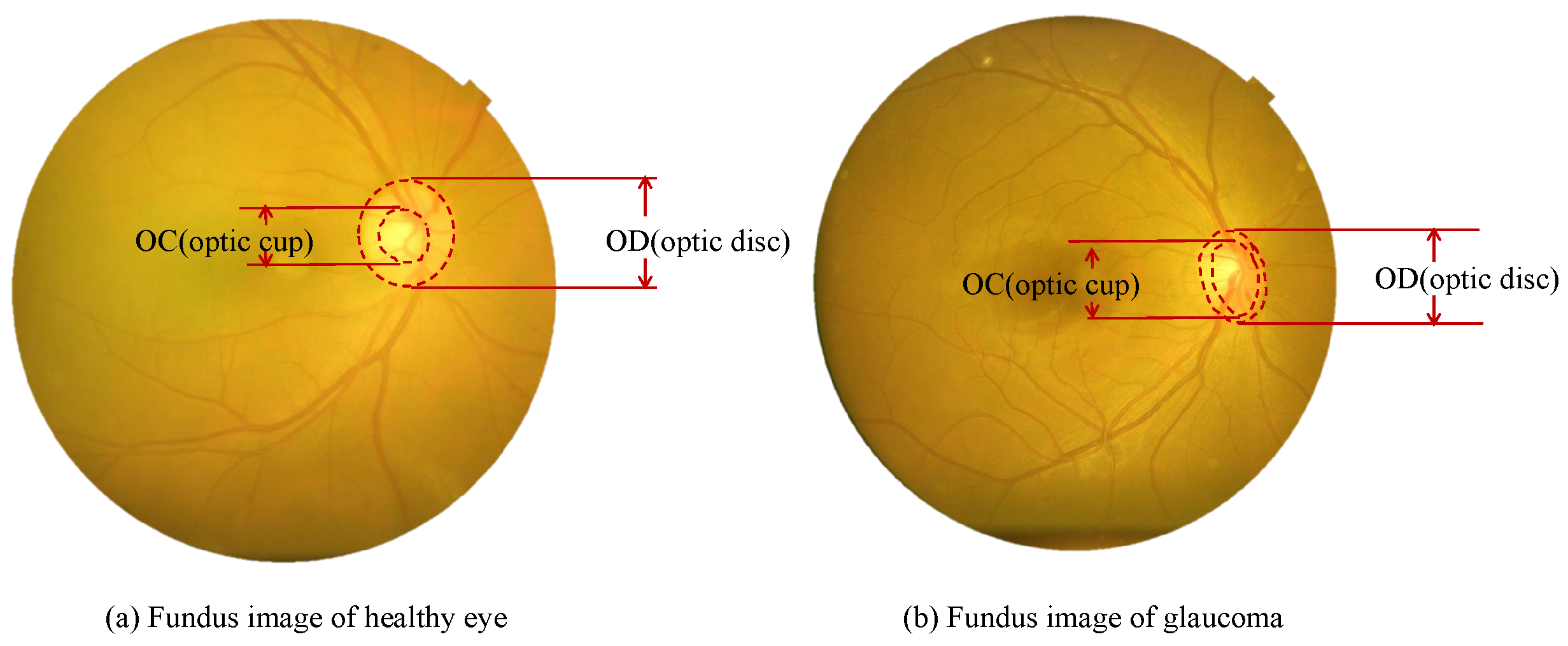
:1. Introduction
- We propose using a novel BEAC-Net network for OD and OC segmentation based on the ACM (adaptive context module), which eliminates noise in critical pixels when fully effective.
- We design an EBPA (efficient boundary pixel attention) module that can impose boundary awareness on the proposed network via cumulative contextual information in the horizontal and vertical directions to enhance pixel-by-pixel feature capture.
- We construct an AFF (attentional feature fusion) module to integrate the feature maps from high-level and low-level features adaptively. Multi-scale hierarchical feature extraction avoids an excessive loss of key information in the original images.
- We provide a high-quality retinal fundus image dataset named the 66 Vision-Tech dataset. The fundus images are from 66 VISION TECH Co., Ltd., No. 9 Jinfeng Road, High-tech District, Suzhou 215163, China.The experiment results demonstrate the good generalization properties of the model.
2. Related Work
3. Methods
3.1. Overview
3.2. Adaptive Context Module
3.3. Adaptive Spatial Pyramid Pooling
3.4. Efficient Boundary Pixel Attention
3.5. Attentional Feature Fusion
| Algorithm 1 Description of the AFF |
|
3.6. Loss Function
4. 66 Vision-Tech Dataset
5. Experiments
5.1. Datasets
- Data annotation. Two ophthalmologists used Labelme to annotate 160 fundus images of the optic disk (OD) and optic cup (OC). In this paper, 140 were randomly selected as the training set and 20 were randomly selected as the test set using the division method following [31].
- Data Augmentation. The fundus images are pre-processed for image defogging and contrast enhancement using the Automatic Color Enhancement (ACE) [32] algorithm, which corrects the final pixel values by calculating the degree of lightness and darkness of the target pixels and the surrounding pixels and their relationship to achieve contrast adjustment of the image. Due to the small number of images, in the experiment, we use random vertical flip, random horizontal flip, and random diagonal flip to every image [33], and one image is expanded to 2 × 2 × 2 = 8 images by expanding the dataset.
- Cropping ROI [34]. A small percentage of the OD area in the fundus images is used to obtain more accurate boundary segmentation of the optic disk and reduce the influence of background noise regions on the segmentation results. The center of the OD is detected by the brightest point in the fundus image as the center of the OD. Then, it performs an external expansion twice the radius of the cropped OD region to obtain the full area of the OD and OC, which is sent to the BEAC-Net model for training and testing. In particular, the cropping images reduce the computing load on the computer and improve the computing efficiency. The labels are cropped into the corresponding ROI simultaneously.
5.2. Implementation Details
5.3. Evaluation Metrics
5.4. Comparison with State-of-the-Art Models
5.5. Results on Cross-Dataset
5.6. Ablation Study
- (1)
- Efficient Boundary Pixel Attention
- (2)
- Attentional Feature Fusion
- (3)
- ASPP influence
- (4)
- Dice Loss
6. Conclusions
Author Contributions
Funding
Institutional Review Board Statement
Informed Consent Statement
Data Availability Statement
Conflicts of Interest
References
- Weinreb, R.N.; Leung, C.K.S.; Crowston, J.G.; Medeiros, F.A.; Friedman, D.S.; Wiggs, J.L.; Martin, K.R. Primary open-angle glaucoma. Nat. Rev. Dis. Prim 2004, 363, 1711–1720. [Google Scholar]
- Herndon; Leon, W. Central corneal thickness as a risk factor for advanced glaucoma damage. Arch. Ophthalmol. 2004, 122, 17–21. [Google Scholar] [PubMed]
- Razzak, M.I.; Naz, S.; Zaib, A. Deep learning for medical image processing: Overview, challenges and the future. In Classification in BioApps: Automation of Decision Making; Springer: Berlin/Heidelberg, Germany, 2018; pp. 323–350. [Google Scholar]
- Feng, Y.; Ji, Y.; Wu, F.; Gao, G.; Gao, Y.; Liu, T.; Liu, S.; Jing, X.Y.; Luo, J. Occluded Visible-Infrared Person Re-Identification. IEEE Trans. Multimed. 2023, 25, 1401–1413. [Google Scholar]
- Liu, Q.; Hong, X.; Ke, W.; Chen, Z.; Zou, B. DDNet: Cartesian-polar Dual-domain Network for the Joint Optic Disc and Cup Segmentation. arXiv 2019, arXiv:1904.08773. [Google Scholar]
- Biswal, B.; Vyshnavi, E.; Sairam, M.V.S.; Rout, K. Robust Retinal Optic Disc and Optic Cup Segmentation via Stationary Wavelet Transform and Maximum Vessel Pixel Sum. Inst. Eng. Technol. 2020, 14, 592–602. [Google Scholar]
- Long, J.; Shelhamer, E.; Darrell, T. Fully Convolutional Networks for Semantic Segmentation. IEEE Trans. Pattern Anal. Mach. Intell. 2015, 39, 640–651. [Google Scholar]
- Ronneberger, O.; Fischer, P.; Brox, T. U-Net: Convolutional Networks for Biomedical Image Segmentation. In Proceedings of the International Conference on Medical Image Computing and Computer-Assisted Intervention, Munich, Germany, 5–9 October 2015; pp. 234–241. [Google Scholar]
- Qin, P.; Wang, L.; Lv, H. Optic Disc and Cup Segmentation Based on Deep Learning. In Proceedings of the Information Technology, Networking, Electronic and Automation Control Conference, Chengdu, China, 15–17 March 2019; pp. 1835–1840. [Google Scholar]
- Zilly, J.; Buhmann, J.M.; Mahapatra, D. Glaucoma detection using entropy sampling and ensemble learning for automatic optic cup and disc segmentation. Comput. Med. Imaging Graph. 2017, 55, 28–41. [Google Scholar]
- Liu, Z.; Yuan, H.; Shao, Y.; Liu, M. ResD-Unet Research and Application for Pulmonary Artery Segmentation. IEEE Access 2021, 9, 67504–67511. [Google Scholar]
- Fu, H.; Cheng, J.; Xu, Y.; Wong, D.W.K.; Liu, J.; Cao, X. Joint Optic Disc and Cup Segmentation Based on Multi-label Deep Network and Polar Transformation. IEEE Trans. Med. Imaging 2018, 37, 1597–1605. [Google Scholar]
- Tabassum, M.; Khan, T.M.; Arsalan, M.; Naqvi, S.S.; Mirza, J. CDED-Net: Joint Segmentation of Optic Disc and Optic Cup for Glaucoma Screening. IEEE Access 2020, 8, 102733–102747. [Google Scholar]
- Huang, Z.; Wang, X.; Huang, L.; Huang, C.; Liu, W. CCNet: Criss-Cross Attention for Semantic Segmentation. In Proceedings of the IEEE/CVF International Conference on Computer Vision, Salt Lake City, UT, USA, 23–18 June 2018; pp. 603–612. [Google Scholar]
- Chen, L.C.; Zhu, Y.; Papandreou, G.; Schroff, F.; Adam, H. Encoder-decoder with atrous separable convolution for semantic image segmentation. In Proceedings of the European Conference on Computer Vision, Munich, Germany, 8–14 September 2018; pp. 801–818. [Google Scholar]
- Dosovitskiy, A.; Beyer, L.; Kolesnikov, A.; Weissenborn, D.; Zhai, X.; Unterthiner, T. Transformers for image recognition at scale. arXiv 2020, arXiv:2010.11929. [Google Scholar]
- Aquino, A.; Gegundez-Arias, M.E.; Marin, D. Detecting the optic disc boundary in digital fundus images using morphological, edge detection, and feature extraction techniques. IEEE Trans. Med. Imaging 2010, 29, 1860–1869. [Google Scholar] [PubMed]
- Chen, L. Weakly Supervised and Semi-Supervised Semantic Segmentation for Optic Disc of Fundus Image. Symmetry 2020, 12, 145. [Google Scholar]
- Sukanya, R. Retinal Blood Vessel Segmentation and Optic Disc Detection Using Combination of Spatial Domain Techniques. Int. J. Comput. Sci. Eng. 2015, 4, 102–109. [Google Scholar]
- Cheng, J.; Liu, J.; Xu, Y. Superpixel Classification Based Optic Disc and Optic Cup Segmentation for Glaucoma Screening. IEEE Trans. Med. Imaging 2013, 32, 1019–1032. [Google Scholar] [PubMed]
- Feng, Y.; Yu, J.; Chen, F.; Ji, Y.; Wu, F.; Liu, S.; Jing, X.Y. Visible-Infrared Person Re-Identification via Cross-Modality Interaction Transformer. IEEE Trans. Multimed. 2022. early access. [Google Scholar] [CrossRef]
- Huang, G.; Liu, Z.; Van Der Maaten, L.; Weinberger, K.Q. Densely connected convolutional networks. In Proceedings of the IEEE Conference on Computer Vision and Pattern Recognition, Honolulu, HI, USA, 21–26 July 2017; pp. 4700–4708. [Google Scholar]
- Gu, Z.; Cheng, J.; Fu, H.; Zhou, K.; Hao, H.; Zhao, Y.; Zhang, T.; Gao, S.; Liu, J. Ce-net: Context encoder network for 2d medical image segmentation. IEEE Trans. Med. Imaging 2019, 38, 2281–2292. [Google Scholar] [PubMed]
- Wang, S.; Yu, L.; Li, K.; Yang, X.; Heng, P.A. DoFE: Domain-oriented Feature Embedding for Generalizable Fundus Image Segmentation on Unseen Datasets. IEEE Trans. Med. Imaging 2020, 39, 4237–4248. [Google Scholar] [PubMed]
- Liu, Z.; Lin, Y.; Cao, Y.; Hu, H.; Wei, Y.; Zhang, Z.; Lin, S.; Guo, B. Swin transformer: Hierarchical vision transformer using shifted windows. In Proceedings of the IEEE/CVF International Conference on Computer Vision, Montreal, QC, Canada, 10–17 October 2021; pp. 10012–10022. [Google Scholar]
- Chen, J.; Lu, Y.; Yu, Q.; Luo, X.; Zhou, Y. TransUNet: Transformers Make Strong Encoders for Medical Image Segmentation. arXiv 2021, arXiv:2102.04306. [Google Scholar]
- Lin, A.; Chen, B.; Xu, J.; Zhang, Z.; Lu, G. DS-TransUNet: Dual Swin Transformer U-Net for Medical Image Segmentation. IEEE Trans. Instrum. Meas. 2022, 71, 3178991. [Google Scholar]
- Azad, R.; Heidari, M.; Shariatnia, M.; Aghdam, E.K.; Karimijafarbigloo, S.; Adeli, E.; Merhof, D. Transdeeplab: Convolution-free transformer-based deeplab v3+ for medical image segmentation. In Proceedings of the Predictive Intelligence in Medicine, Singapore, 22 September 2022; Springer: Berlin/Heidelberg, Germany, 2022; pp. 91–102. [Google Scholar]
- Fumero, F.; Alayon, S.; Sanchez, J.L.; Sigut, J.; Gonzalez-Hernandez, M. RIM-ONE: An open retinal image database for optic nerve evaluation. In Proceedings of the 24th International Symposium on Computer-Based Medical Systems (CBMS), Bristol, UK, 27–30 June 2011; pp. 1–6. [Google Scholar]
- Sivaswamy, J.; Krishnadas, S.R.; Chakravarty, A.; Joshi, G.D.; Ujjwal. A Comprehensive Retinal Image Dataset for the Assessment of Glaucoma from the Optic Nerve Head Analysis. JSM Biomed. Imaging Data Pap. 2015, 2, 1004. [Google Scholar]
- Wang, S.; Yu, L.; Yang, X.; Fu, C.W.; Heng, P.A. Patch-based output space adversarial learning for joint optic disc and cup segmentation. IEEE Trans. Med. Imaging 2019, 38, 2485–2495. [Google Scholar] [CrossRef]
- Getreuer, P. Automatic color enhancement (ACE) and its fast implementation. Image Process. Line 2012, 2, 266–277. [Google Scholar] [CrossRef]
- Fu, J.; Liu, J.; Tian, H.; Li, Y.; Bao, Y.; Fang, Z.; Lu, H. Dual attention network for scene segmentation. In Proceedings of the IEEE/CVF conference on computer vision and pattern recognition, Seattle, WA, USA, 13–19 June 2019; pp. 3146–3154. [Google Scholar]
- Nieto-Castanon, A.; Ghosh, S.S.; Tourville, J.A.; Guenther, F.H. Region of interest based analysis of functional imaging data. Neuroimage 2003, 19, 1303–1316. [Google Scholar] [CrossRef]
- Cao, H.; Wang, Y.; Chen, J.; Jiang, D.; Zhang, X.; Tian, Q.; Wang, M. Swin-unet: Unet-like pure transformer for medical image segmentation. In Proceedings of the European Conference on Computer Vision, Tel Aviv, Israel, 23–24 October 2022; pp. 205–218. [Google Scholar]
- Chen, L.C.; Papandreou, G.; Kokkinos, I.; Murphy, K.; Yuille, A.L. DeepLab: Semantic Image Segmentation with Deep Convolutional Nets, Atrous Convolution, and Fully Connected CRFs. IEEE Trans. Pattern Anal. Mach. Intell. 2016, 40, 834–848. [Google Scholar]


| Dataset | Year of Publication | Total Number | Number of Training Sets | Number of Testing Sets |
|---|---|---|---|---|
| DRISHTI-GS | 2017 | 101 | 50 | 51 |
| RIM-ONE-v3 | 2021 | 159 | 140 | 19 |
| 66 Vision-Tech | 2023 | 150 | 130 | 20 |
| Method | RIM-ONE-v3 Dataset | DRISHTI-GS Dataset | ||||||
|---|---|---|---|---|---|---|---|---|
| OD | OC | OD | OC | |||||
| Dice | IoU | Dice | IoU | Dice | IoU | Dice | IoU | |
| U-Net [8] | 0.7351 | 0.8206 | 0.7176 | 0.6633 | 0.7887 | 0.8206 | 0.7376 | 0.7533 |
| Deeplabv3+ [15] | 0.7467 | 0.8344 | 0.7236 | 0.6701 | 0.7861 | 0.8344 | 0.7336 | 0.7001 |
| CE-Net [23] | 0.7632 | 0.8478 | 0.7592 | 0.6732 | 0.7932 | 0.8478 | 0.7492 | 0.7532 |
| M-Met [12] | 0.7696 | 0.8114 | 0.7348 | 0.6900 | 0.8026 | 0.8114 | 0.7648 | 0.7300 |
| Ensemble CNN [10] | 0.8132 | N/A | 0.7240 | N/A | 0.8120 | N/A | 0.7740 | N/A |
| U-shaped [33] | 0.8344 | N/A | 0.7564 | N/A | 0.8361 | N/A | 0.7764 | N/A |
| Robust [6] | 0.8410 | 0.8256 | 0.7129 | 0.6633 | 0.8310 | 0.8256 | 0.7945 | 0.7429 |
| Swin-Unet [35] | 0.8412 | 0.8101 | 0.7332 | 0.6633 | 0.8582 | 0.8101 | 0.7822 | 0.7532 |
| Our | 0.8582 | 0.8385 | 0.7333 | 0.6633 | 0.8614 | 0.8385 | 0.8087 | 0.7633 |
| Method | OD | OC | ||||
|---|---|---|---|---|---|---|
| Dice | IoU | HD | Dice | IoU | HD | |
| U-Net [8] | 0.6948 | 0.7256 | 35.82 | 0.6515 | 0.7534 | 39.60 |
| Deeplab [36] | 0.7231 | 0.7512 | 29.74 | 0.6752 | 0.7655 | 33.52 |
| Deeplabv3+ [15] | 0.7554 | 0.7440 | 21.55 | 0.6836 | 0.7521 | 26.23 |
| M-Met [12] | 0.7675 | 0.7778 | 22.16 | 0.6872 | 0.7678 | 30.25 |
| Trans-Unet [26] | 0.7947 | 0.8065 | 18.75 | 0.7102 | 0.7763 | 21.85 |
| Swin-Unet [35] | 0.8149 | 0.8052 | 12.32 | 0.7441 | 0.7815 | 15.65 |
| Our | 0.8267 | 0.8138 | 8.63 | 0.8057 | 0.7858 | 9.59 |
| EBPA | AFF | ASPP | OD | OC | ||||
|---|---|---|---|---|---|---|---|---|
| Dice | IoU | HD | Dice | IoU | HD | |||
| - | - | - | 0.7523 | 0.7636 | 35.82 | 0.7426 | 0.7108 | 33.56 |
| ✓ | - | - | 0.7630 | 0.7841 | 22.23 | 0.7654 | 0.7453 | 25.43 |
| - | ✓ | - | 0.7837 | 0.7947 | 23.36 | 0.7742 | 0.7547 | 25.50 |
| - | - | ✓ | 0.8148 | 0.7952 | 21.47 | 0.7759 | 0.7557 | 25.21 |
| ✓ | ✓ | - | 0.8156 | 0.8017 | 15.23 | 0.7867 | 0.7712 | 17.78 |
| ✓ | ✓ | ✓ | 0.8267 | 0.8138 | 8.63 | 0.8057 | 0.7858 | 9.59 |
| Method | Dice | IoU | ||
|---|---|---|---|---|
| OD | OC | OD | OC | |
| BEAC-Net + | 0.8203 | 0.8059 | 0.8121 | 0.7767 |
| BEAC-Net + + | 0.8367 | 0.8157 | 0.8238 | 0.7958 |
Disclaimer/Publisher’s Note: The statements, opinions and data contained in all publications are solely those of the individual author(s) and contributor(s) and not of MDPI and/or the editor(s). MDPI and/or the editor(s) disclaim responsibility for any injury to people or property resulting from any ideas, methods, instructions or products referred to in the content. |
© 2023 by the authors. Licensee MDPI, Basel, Switzerland. This article is an open access article distributed under the terms and conditions of the Creative Commons Attribution (CC BY) license (https://creativecommons.org/licenses/by/4.0/).
Share and Cite
Jiang, L.; Tang, X.; You, S.; Liu, S.; Ji, Y. BEAC-Net: Boundary-Enhanced Adaptive Context Network for Optic Disk and Optic Cup Segmentation. Appl. Sci. 2023, 13, 10244. https://doi.org/10.3390/app131810244
Jiang L, Tang X, You S, Liu S, Ji Y. BEAC-Net: Boundary-Enhanced Adaptive Context Network for Optic Disk and Optic Cup Segmentation. Applied Sciences. 2023; 13(18):10244. https://doi.org/10.3390/app131810244
Chicago/Turabian StyleJiang, Lincen, Xiaoyu Tang, Shuai You, Shangdong Liu, and Yimu Ji. 2023. "BEAC-Net: Boundary-Enhanced Adaptive Context Network for Optic Disk and Optic Cup Segmentation" Applied Sciences 13, no. 18: 10244. https://doi.org/10.3390/app131810244
APA StyleJiang, L., Tang, X., You, S., Liu, S., & Ji, Y. (2023). BEAC-Net: Boundary-Enhanced Adaptive Context Network for Optic Disk and Optic Cup Segmentation. Applied Sciences, 13(18), 10244. https://doi.org/10.3390/app131810244