Space–Time Stress Variations near the East Anatolian Fault Zone and the Triggering Relationship of Earthquakes

Abstract

Several major earthquakes have taken place near the East Anatolian fault zone (EAFZ) in history. Despite extensive research on the Coulomb stress changes associated with these earthquakes, there remains a paucity of studies examining the spatial and temporal distribution of Coulomb stress near the East Anatolian fault zone over extended periods. This study investigates the changes in Coulomb stress induced by significant earthquakes (≥6 Mw) near the EAFZ from 1986 to 2023. High-stress changes (1.5–2.5 bar) were observed along the fault’s northeastern and southwestern segments, indicating a high likelihood of future seismicity. We also found that the three major earthquakes between 1986 and 2003 had little impact on subsequent major seismic events in the vicinity. However, the 2020 Mw 6.8 earthquake generated a Coulomb stress increment exceeding 0.1 bar, which influenced nearby seismic activity for two years. This suggests that the 2023 major earthquakes were likely facilitated by this stress change. Parameter sensitivity analysis shows fault strikes significantly affect calculations, highlighting the importance of accurate source mechanisms for reliable results. The findings of this study offer critical insights for seismologists and geophysicists aiming to refine earthquake-triggering models and stress transfer mechanisms. Civil engineers and urban planners can utilize the identified high-stress zones to prioritize seismic retrofitting of infrastructure.

1. Introduction

A significant portion of Turkish territory is proximate to major fault systems, primarily influenced by the East Anatolian fault zone (EAFZ) and the North Anatolian fault zone (NAFZ). Both the subduction of the African plate and the lateral movement and convergent collision of the Arabian and Eurasian tectonic plates created these fault zones, which meet at Karliova in northern Turkey. With a displacement rate of 21–25 mm/year, the NAFZ is classified as a dextral strike-slip fault zone, whereas the EAFZ is classified as a sinistral strike-slip fault zone, with movement at a rate of 4–10 mm/year [1,2,3,4]. Historically, seismic activity has been more prevalent near the NAFZ than in the EAFZ over the past century. However, there were two significant earthquakes within the EAFZ on 6 February 2023. At 04:17 local time, the first earthquake (7.7 Mw) struck. Its hypocenter was situated at 37.288° N, 37.043° E with an 8.6 km depth [5]. The second earthquake (7.6 Mw) happened at 13:24 local time. Its hypocenter was situated at 38.089° N, 37.239° E with a 7 km depth [5]. Over 50,000 people lost their lives as a result of these two devastating earthquakes [6]. The devastation and losses caused by major earthquakes underscore the critical need for effective methods to assess seismic hazards. Coulomb stress changes ($∆CFS$) are considered to be an important factor influencing seismic activity [7]. Therefore, we want to evaluate the Coulomb stress changes near the EAFZ to achieve an accurate understanding of the seismic risk in this area.

When stress accumulates on a fault and exceeds a certain threshold, it leads to rupture deformation and initiates seismic activity. Following an earthquake event, the surrounding stress conditions undergo readjustment. While stresses in the Earth’s crust are generally alleviated following an earthquake, there are instances where stresses in specific regions intensify, ultimately leading to fault destabilization and rupture in those areas [8]. This phenomenon, known as stress triggering [9], occurs especially when an earthquake promotes subsequent seismic events due to elastic dislocations during the coseismic rupture phase [10]. Elastic dislocations caused by earthquakes, viscoelastic relaxation due to sliding, and stress changes from tectonic movements all contribute to the triggering of subsequent seismic activity [11].

Extensive research has focused on how static Coulomb stress alterations caused by earthquakes influence subsequent fault ruptures. Rybicki initially investigated the influence of stresses generated by the main rupture on aftershocks using dislocation theory [12]. Using the Coulomb failure criterion, Das and Scholz investigated how co-seismic static Coulomb stress changes trigger subsequent earthquakes in nearby areas [13]. Subsequently, Stein and Lisowski applied a similar methodology to investigate the connection between static stress triggering and the 1979 Homestead Valley mainshock and its aftershocks in California [14]. According to their findings, most aftershocks centered in regions where the primary shock caused a significant increase in static Coulomb stress.

However, the seismological community did not highlight the significance of static stress-triggered effects on the surrounding stress field because the magnitude of static Coulomb stress changes from previous studies was significantly smaller than that of the Stress Drop [15]. In their analysis of the effects of static Coulomb stress on the 1992 7.3 Mw Landers earthquake on the San Andreas Fault, Stein et al. emphasized the part foreshocks play in causing the mainshock and the mainshock’s subsequent effect on aftershocks [16]. This led scholars to focus on studies related to earthquake stress triggering. In Southern California, Anderson et al. found that large earthquakes on the northern San Jacinto Fault could cause cascading ruptures in the Sierra Madre–Cucamonga system by mimicking dynamic shear stress variations between strike-slip and reverse-strike faults and static Coulomb stress changes [17]. Pollitz et al. assessed the stress changes related to both co-seismic and post-seismic deformation following two major earthquakes of 9.2 Mw and 8.7 Mw on the Great Sumatra Retroflex Fault based on the Coulomb failure stress theory [18]. Shan et al. examined the effects of the Wenchuan earthquake (7.9 Mw) by simulating Coulomb stress changes along the Xianshuihe–Xiaojiang Fault System [19].

A considerable body of research has shown that both the Coulomb failure stress theory and the stress trigger theory serve as effective indicators for evaluating seismic hazards [20,21,22,23,24]. The EAFZ has not recorded a significant number of large earthquakes exceeding 7 Mw in the past century. The 7.7 Mw and 7.6 Mw earthquakes of 6 February 2023, were bound to release much energy into the surrounding area. This energy will likely disrupt the stress balance on the surrounding faults, triggering new earthquakes. Previous studies on major earthquakes near the EAFZ have focused solely on Coulomb stress changes induced by individual large seismic events [1,21,25,26]. Current research in the EAFZ region remains limited regarding the long-term spatiotemporal evolution of Coulomb stresses. To address this gap, we investigate Coulomb stress variations generated by earthquakes exceeding magnitude 6 near the EAFZ from 1986 to 2023. Our analysis examines the spatiotemporal evolution of Coulomb stress in this region and evaluates potential triggering relationships between successive earthquakes.

While there are many studies that use machine learning techniques to assess seismic risk, such as Kazemi et al.’s study of machine learning-based seismic vulnerability and susceptibility assessment of reinforced concrete buildings, the study in this study differs from such studies in both scope and methodology [27]. While Kazemi et al. [27] utilized machine learning to predict structural responses to seismic events, our work employs geophysical modeling and stress tensor inversion to analyze the spatial and temporal evolution of Coulomb stress changes induced by historical earthquakes. This allows us to assess how stress changes influence the likelihood of future seismic events, providing a complementary perspective to structural-based risk assessments. By integrating stress tensor inversion and Coulomb stress calculations, we offer a more comprehensive understanding of the seismic hazard in the EAFZ region, which is critical for both structural engineering and geophysical earthquake forecasting.

To investigate the Coulomb stress development in the vicinity of the EAFZ, we selected earthquakes with magnitudes exceeding 6 Mw that occurred between 1986 and 2023 for our analysis. The $∆CFS$ around the EAFZ is analyzed from both spatial and temporal aspects. In addition, we calculate the specific values of $∆CFS$ induced by these significant earthquakes (6 Mw) for subsequent seismic events and discuss their impact on ensuing seismicity.

2. Background

The EAFZ constitutes a significant tectonic feature that delineates the boundary between the Anatolian and Arabian tectonic plates (see Figure 1a). It is a 700 km-long left-lateral strike-slip fault system that starts in the northeastern Karlıova triple junction and joins the NAFZ [28]. It continues southwestward to the Mediterranean Sea, ultimately connecting with the Dead Sea Fault [4,29,30]. Wollin et al. used seismic databases from 2006 to 2016 to examine the stress tensor within the Marmara area surrounding the NAFZ in Turkey [31]. The findings showed that the region’s tectonic system was defined by normal and strike-slip faults, with tensile stress present throughout [31]. Using seismic databases from 1976 to 2024, Ma et al. investigated the stress tensor in the area around the EAFZ in Turkey and demonstrated that strike-slip and reversal faults are prevalent in this area [32]. Despite its historically lower seismicity relative to the NAFZ, the EAFZ possesses the capacity to generate significant earthquakes [33,34,35]. The Arabian Plate’s northward movement toward the Eurasian Plate affects the EAFZ’s overall tectonic structure [30,36]. The Anatolian microplate is encouraged to extrude westward by the compressional pressures created by this tectonic action [28,37]. Consequently, the tectonic dynamics associated with the EAFZ render it a significant subject of investigation within the fields of seismology and geophysics [38,39,40,41,42].

Eight earthquakes (≥6 Mw) have occurred in the vicinity of the EAFZ in the last 40 years (Figure 1b). The southern portion of the EAFZ experienced a 7.7 Mw earthquake on 6 February 2023, at 04:17 local time [5]. Then, at 13:24 local time, another 7.6 Mw earthquake took place, with the distance of the two epicenters approximately 100 km apart [5]. The first large earthquake ruptured from its epicenter in a northeast-to-southwest direction, while the second ruptured in an east–west direction. The earthquake rupture zone crossed the border between Türkiye and Syria, causing devastating damage in both countries [6]. This devastating double quake also triggered two major aftershocks of 6.6 Mw and 6.4 Mw. Four earthquakes occurring in such proximity produced more catastrophic damage than the previous four earthquakes greater than 6 Mw.

3. Materials and Methods

3.1. Coulomb Failure Stress Changes

The substantial energy released during earthquakes influences the stress conditions along fault surfaces, thereby facilitating or impeding subsequent fault movement to varying degrees [45]. Specifically, we use Coulomb failure stress (CFS) to investigate the stress relationships in the Earth’s crust:

$$CFS=\left|\tau \right|-[S-\mu ({\sigma }_n+P_r\left)\right],$$

(1)

where $\tau$ is the shear on the fault plane, $S$ is the cohesive stress in the fault medium, $\mu$ is the internal friction coefficient, ${\sigma }_n$ is the normal stress on the fault plane, and $P_r$ is the pore pressure on the fault plane. As $\left|\tau \right|$ moves closer to $S-\mu ({\sigma }_n+P_r)$, the rock breaks up more easily. The Coulomb failure criterion was derived by measuring the shear and normal stresses applied to rock samples in the laboratory [46]. However, in the Earth’s crust, absolute stress values are difficult to measure. Although we may not know the absolute value of stress on a fault, we can calculate the Coulomb stress changes using the following expression by assuming that $S$ and $\mu$ do not vary with time [45,46,47]:

$$∆CFS=∆\tau +\mu ({∆\sigma }_{\mathrm{n}}+∆P_r),$$

(2)

where $∆\tau$ is the shear stress variation, and ${∆\mathsf{\sigma }}_{\mathrm{n}}$ is the normal stress variation. After the change in static stress and the free-flowing fluid, the change in pore pressure is defined as

$$∆P_r=-B{\displaystyle \frac{{∆\sigma }_{ii}}{3}},$$

(3)

where B is the Skempton coefficient, and ${∆\sigma }_{ii}$ is the diagonal sum of the stress tensor, i.e., ${∆\sigma }_{ii}={∆\sigma }_{11}+{∆\sigma }_{22}+{∆\sigma }_{33}$. If ${∆\sigma }_{11}={∆\sigma }_{22}={∆\sigma }_{33}$, then ${\displaystyle \frac{{∆\sigma }_{ii}}{3}}={∆\sigma }_{\mathrm{n}}$, at which point (King et al., 1994 [45])

$$∆CFS=∆\tau +\mu \prime {∆\sigma }_{\mathrm{n}},$$

(4)

where $\mu \prime$ is the effective coefficient of friction, which takes values in the range 0–0.8.

When $∆CFS>0$, it indicates that the fault is more prone to slip, and conversely, when $∆CFS<0$, it indicates that the fault becomes more stable. Aftershocks are triggered when $∆CFS$ > 0.1 bar (Harris et al., 1995 [48]; Harris & Simpson, 1998 [49]; Stein, 1999 [47]). In this study, we perform $∆CFS$ calculations using Coulomb 3.4 software based on Okada in an elastic half-space with uniformly isotropic elastic properties [50,51,52].

3.2. Stress Tensor Inversion

Based on the theory of Coulomb failure stress changes, we need the stress tensor of the region where the source fault is located to calculate the $∆CFS$ value of the receiver fault. The stress tensor is a tool used to generalize the state of a regional stress field. If we consider a point as an infinitesimal cube, then the traction force acting on this point can be split into three mutually perpendicular planes. By this method, the force acting on a point is split into nine components:

$$\left[\begin{array}{ccc}{\sigma }_{xx}& {\sigma }_{xy}& {\sigma }_{xz}\\ {\sigma }_{yx}& {\sigma }_{yy}& {\sigma }_{yz}\\ {\sigma }_{zx}& {\sigma }_{zy}& {\sigma }_{zz}\end{array}\right],$$

(5)

where ${\sigma }_{xx}$, ${\sigma }_{yy}$, and ${\sigma }_{zz}$ are normal stresses, and the other six components are shear stresses. Shear stress components with opposite subscripts are equal in magnitude and opposite in direction. Therefore, by knowing the six components, we can determine a stress tensor. During the calculation of $∆CFS$, we need directions of the three principal stress axes (${\sigma }_{xx}$, ${\sigma }_{yy}$, ${\sigma }_{zz}$) in the region where the source fault is located. Usually, we specify ${\sigma }_1>{\sigma }_2>{\sigma }_3$ based on the magnitudes of the principal stresses. The stress ratio R defines the relationship between the magnitudes of the three principal stresses as follows:

$$R={(\mathsf{\sigma }}_1-{\mathsf{\sigma }}_2)/({\mathsf{\sigma }}_1-{\mathsf{\sigma }}_3),$$

(6)

The prevailing stress tensor inversion techniques are performed using the focal mechanisms [53,54,55,56,57]. The fault plane tangential traction is often assumed to be parallel to the fault slide direction, and the research area’s stress field is assumed to be uniform [58,59]. In this study, we used STRESSINVERSE to calculate the stress tensor, which was proposed by Vavryčuk [57]. This approach inverts jointly for stress and fault orientations and can eliminate errors due to an incorrect selection of fault planes. The accuracy of this method was tested by Vavryčuk [57], which showed that the introduction of the fault instability criterion improves the accuracy of the linear inversion and removes the effect of fault uncertainty on the calculation results. The formula for determining the instability of a fault is as follows:

$$I={\displaystyle \frac{\tau -\mu (\sigma -1)}{\mu +\sqrt{1+{\mu }^2}}},$$

(7)

where

$$\mathsf{\tau }=\sqrt{n_1^2+(1-2R)n_2^2+n_3^2-{\left[n_1^2+(1-2R)n_2^2-n_3^2\right]}^2},$$

(8)

n_i are the components of the fault normal n (i = 1, 2, 3), $\mathsf{\mu }$ is the fault friction, and R is the stress ratio defined in Equation (1).

The value of fault instability I range from 0 to 1. The fault is considered most stable when I = 0 and most unstable when I = 1. The most unstable fault is the principal fault, the optimally oriented fault for shear faulting.

This is how the fault instability criterion-based stress inversion operates. First, Michael’s approach [56,60] is used to construct the stress tensor, and fault planes are chosen at random from nodal planes supplied by focal mechanisms. Second, the nodal planes with the highest fault instability are known as fault planes based on the recovered stress. Third, using the fault plane orientations determined by the fault instability criterion, the stress inversion is carried out once more. The procedure is continued until the final stress model is reached by the inversion.

3.3. Data

We used 692 focal mechanisms in total to calculate the stress tensor in the study area (35–41° E and 36–39° N) from the ISC Bulletin [61,62] and the Disaster and Emergency Management Authority (AFAD)—Turkish Earthquake Data Center System Regulation (see Table S1 in Supplementary Materials). In addition, we also employed 164 focal mechanisms of seismic events (≥3 Mw) in the range of 35–41° E and 36–39° N from 21 February 2023 to 12 April 2024 from AFAD. The purpose is to explore what effects existed on subsequent seismic events around Türkiye from the massive earthquakes on February 6 and what interrelationships existed between subsequent earthquakes.

To calculate the principal stress directions needed for the $∆CFS$ calculations, we input the above 692 focal mechanisms into the STRESSINVERSE (Version 1.1.3) codes for the computation. Using the STRESSINVERSE calculation requires several parameters to be set. The number of random noise realizations for estimating the accuracy was set to 100. The standard deviation of the normal distribution of the errors in the noise estimates of the focal mechanisms was set to 5°. The number of iterations of the stress inversion was set to 6, and the number of initial stress inversions with a random choice of faults was set to 10. The friction values ranged from 0.4 to 1 with a step of 0.05. After calculating the stress tensor of the study area, we chose the commonly used effective friction coefficient of 0.4 to calculate the $∆CFS$ [46]. Previous studies have shown that $∆CFS$ calculations are not sensitive to the effective friction coefficient [63]. We estimate the length and width of the faults based on Wells and Coppersmith’s empirical magnitude–area relationship [64]. The fault parameters we used are shown in Table S2 in the Supplementary Materials. We decided to assume that the earthquake originated in the fault’s geometric center. We create source faults in Coulomb 3.4 using the “Create Source Faults from CMT Information” approach. In this way, we can compute the fault’s right-lateral slip and reverse slip by inputting the strike, dip, rake, and Mw information. It is worth noting that only source faults have slips, while receiver faults have no slips. When we want a fault to act as a receiver fault, we need to set its right-lateral slip and reverse slip to 0.

4. Results

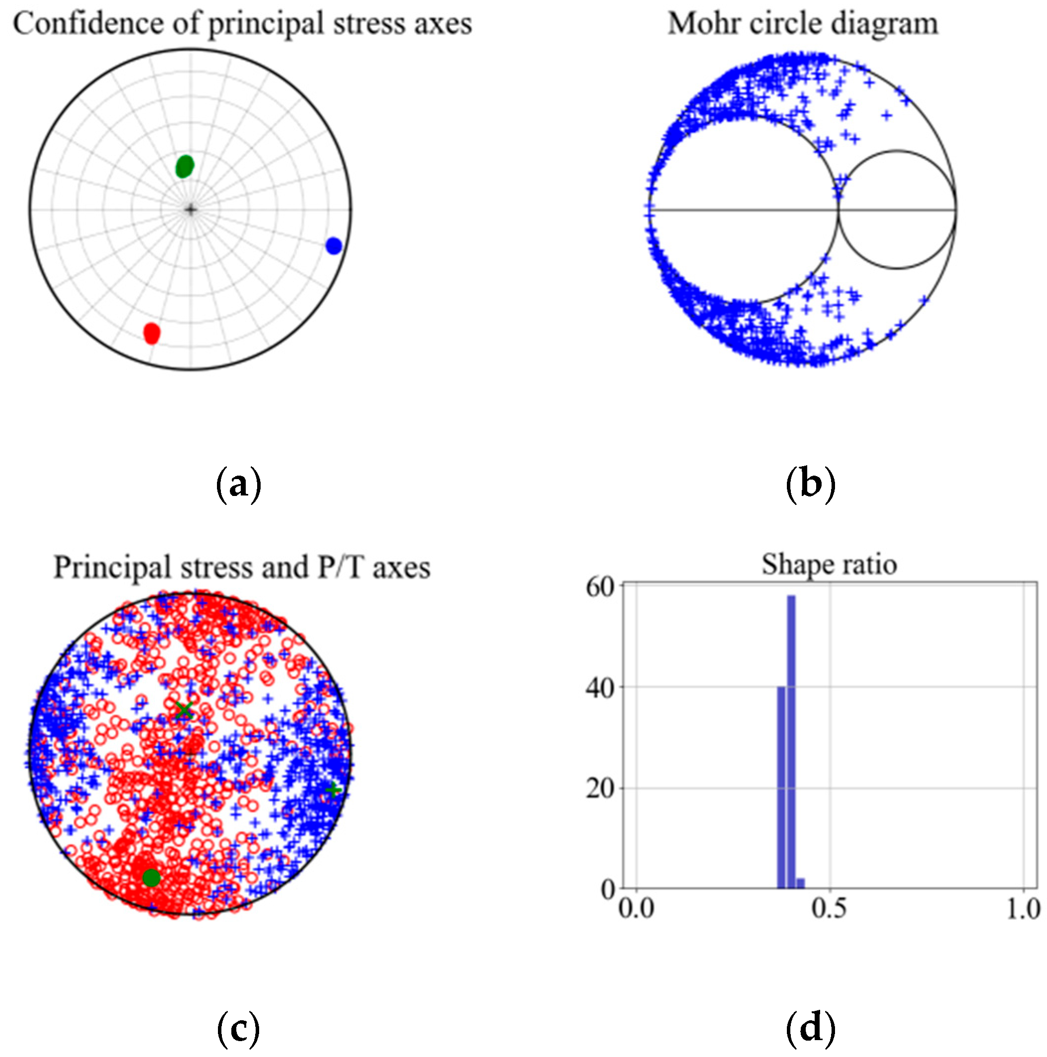
4.1. Results of Stress Tensor Inversion

The results of the stress tensor model using STRESSINVERSE are shown in Figure 2. Calculations in the study area show a typical stress state of a strike-slip fault. The maximum principal stress axis (S1) was oriented in the SWS-NEN direction, while the intermediate principal stress (S2) exhibited a near-vertical alignment. The minimum principal stress axis (S3) was in the ESE-WNW direction. The R-value was 0.384 according to the calculation results. The specific orientation of the principal stress axes and the six components of the stress tensor as well as two principal focal mechanisms found for the retrieved optimum stress tensor are shown in

Table 1. The results were calculated by STRESSINVERSE.

Azimuth1	Plung1	Azimuth2	Plung2	Azimuth3	Plung3
197.3915	20.51909	352.331	67.5516	104.1035	8.712759
See	Sen	Seu	Snn	Snu	Suu
−0.646715	−0.442439	0.181673	0.851544	0.236023	−0.204829
Strike1 (°)	Dip1 (°)	Rake1 (°)	Strike2 (°)	Dip2 (°)	Rake2 (°)
347.600	88.049	−157.630	221.980	72.523	−14.314

. Azimuth1 and plunge1 are the azimuth and plunge of S1. Azimuth2 and plunge2 are the azimuth and plunge of S2. Azimuth3 and plunge3 are the azimuth and plunge of S3. See, Sen, Seu, Snn, Snu, and Suu are the stress tensors calculated by STRESSINVERSE. Strike1, Dip1, Rake1, Strike2, Dip2, and Rake2 are the two principal focal mechanisms found for the retrieved optimum stress tensor. These results are input data for the $∆CFS$ calculation.

4.2. Results of Coulomb Failure Stress Changes

The resolved principal stress axes’ directions were used for the $∆CFS$ calculations by the method described in Section 3.1.

Table 2. Seismic information is used to calculate Coulomb stress changes.

Date	Latitude (°N)	Longitude (°E)	Depth (km)	Magnitude (Mw)	Strike (°)	Dip (°)	Rake (°)
05-05-1986	37.72	37.70	15.0	6.0	215.9670	81.8935	105.2100
27-06-1998	36.87	35.58	29.5	6.2	168.6750	53.4500	68.4607
01-05-2003	39.04	40.53	15.0	6.3	43.6277	35.1118	119.0660
24-01-2020	38.36	39.06	8.1	6.8	248.0000	76.0000	1.0000
06-02-2023	37.29	37.04	8.6	7.7	233.0000	74.0000	18.0000
06-02-2023	37.30	36.92	6.2	6.6	186.3580	42.2270	−30.5910
06-02-2023	38.09	37.24	7.0	7.6	89.7601	84.2631	17.0882
20-02-2023	36.04	36.02	21.7	6.4	214.0000	57.0000	−44.0000

presents information regarding the eight earthquakes that were incorporated into the calculations. As shown in Figure 3, we calculated the $∆CFS$ induced by eight earthquakes larger than 6 Mw in the study area from 1986 to 2023 (specific calculated values see Tables S3 and S4 in Supplementary Materials). The upper section of the figure presents the $∆CFS$ resulting from earthquakes occurring at a depth of 10 km below the surface, while the lower section depicts the $∆CFS$ along the vertical plane of the AB line indicated in the upper section. Figure 3a illustrates the $∆CFS$ associated with four earthquakes of magnitudes greater than 6 Mw that occurred in eastern Türkiye between 1986 and 2020. Notably, since none of these earthquakes overcame a magnitude of 7 Mw, the resultant $∆CFS$ was relatively modest. The vertical plane representation reveals that the $∆CFS$ from the earthquakes of 1986 and 1998 only influenced the subsurface to a depth of 20 km. The 1986 earthquake, with a magnitude of 6.0 Mw, generated a $∆CFS$ averaging 0.41 bar at a depth of 10 km. In the AB vertical plane, positive $∆CFS$ values were predominantly located closer to the surface, averaging at 0.96 bar, while the averaging negative value was −0.93 bar. The 6.2 Mw earthquake in 1998 did not produce extensive areas of significant positive or negative $∆CFS$ at the 10 km depth, with mean positive and negative values of 0.33 bar and −0.77 bar, respectively. However, the AB vertical plane exhibited a substantial area of elevated positive $∆CFS$ values above the 10 km depth, reaching a mean value of about 2.2 bar, indicating a heightened likelihood of subsequent seismic activity near the epicenter at depths up to 10 km. Conversely, negative $∆CFS$ values were primarily located below the 10 km depth, with an averaging value of −0.41 bar. The 2003 earthquake, with a magnitude of 6.3 Mw, demonstrated a slightly broader range of effects, yet did not extend beyond 30 km into the subsurface. It produced an average $∆CFS$ value of 0.75 bar on the plane at 10 km. The Coulomb stress changes induced by this earthquake show two regions of high values with a mean of about 2.8 bar near the surface not more than 10 km below ground. The 2020 earthquake with 6.8 Mw, exhibited a more extensive influence, extending to a depth of 50 km. Near the epicenter of this earthquake, where the $∆CFS$ is higher than 1 bar, the average value reached about 5.4 bar. A significant area of increased $\text{Coulomb} \text{failure} \text{stress}$ was identified in proximity to the source, oriented along the NE-SW direction, although a smaller region of negative $∆CFS$ values was also present nearby, with an average of about −0.44 bar.

Figure 3b shows the $∆CFS$ resulting from four earthquakes with magnitudes exceeding 6 Mw that occurred in 2023. Notably, the seismic events with magnitudes of 7.7 Mw and 7.6 Mw induce significantly larger ranges of $∆CFS$, extending down to depths of 100 km. It is also important to notice that the $∆CFS$ produced close to the A-end primarily serves to prevent further earthquakes from occurring within the AB vertical plane. The $∆CFS$ values are very high in the 200 km long range along the AB plane close to the 7.7 Mw event, with a mean value of 3.77 bar, which is similar to the 3 bar calculated by Stein et al. [65]. This suggests that the 7.7 Mw earthquake triggered the 7.6 Mw event. The average $∆CFS$ value induced by the 7.7 Mw and the 7.6 Mw earthquakes in the study region reached 4.95 bar at 10 km depth. In the northwest of the study area, there is an area of negative $∆CFS$ with a mean value of −0.25 bar. The frequency of seismic activity in this region will decrease in the future, as suggested by Stein et al. [65]. There is also a small area of negative $∆CFS$ in the AB vertical plane near the B side with a mean value of -0.52 bar.

Figure 3c shows the $∆\mathrm{C}\mathrm{F}\mathrm{S}$ generated by eight earthquakes greater than 6 Mw from 1986 to 2023 together. The 6.3 Mw earthquake in 2003 does not show a significant difference compared to Figure 4a because its source is far from the other events. The 6.2 Mw earthquake in 1998 and the 6.8 Mw earthquake in 2020 showed a more pronounced difference than the separate effects. In the plan view at a 10 km depth, the seismic source of the 6.2 Mw event in 1998 affected the northwest region to a greater extent than when the event acted alone. A zone of Coulomb stress decrease occurs to the west of the epicenter of the 2020 6.8 Mw event under joint action compared to separate effects. The extent of the decrease in Coulomb stress at the northeast of the epicenter is reduced, and the extent of Coulomb stress increase is extended. The $∆CFS$ generated by the four events in 2023 reveals a zone of decreasing Coulomb stress in the AB vertical near the B side, but adding the 2020 6.8 Mw earthquake to the calculation reveals that the Coulomb stress turns out to be increasing in this region.

Figure 4 illustrates the $∆CFS$ induced by eight earthquakes on the vertical plane at different latitudes (specific calculated values see Table S5 in Supplementary Materials). Column (a) represents the $∆CFS$ induced by four earthquakes during the period 1986–2020; column (b) represents the $∆CFS$ generated by four earthquakes occurring in 2023; and column (c) represents the $∆CFS$ produced by eight earthquakes combined. An observation of the 39° N vertical plane reveals that the 2023 earthquakes reduced the original stress-increasing area in the 39° E–40° E range and created a stress-reducing area. The large Coulomb stress change area in the 39° N vertical plane is concentrated in the 40° E–41° E range and was induced by the 6.3 Mw earthquake in 2003. The mean positive $∆CFS$ in the 40° E–41° E range of 39° N vertical plane is about 0.86 bar, and the mean negative $∆CFS$ is about −0.97 bar.

The 2023 earthquake produced enormous Coulomb stress changes in the 38.5° N vertical over a range of 35° E–39° E, with a major Coulomb stress increase induced close to the west and a primary Coulomb stress reduction zone close to the east. However, the more extensive Coulomb stress changes in this vertical plane were induced by the 2020 6.8 Mw earthquake with averaging positive and negative $∆CFS$ values of about 0.47 bar and −0.36 bar, respectively. The $∆CFS$ map for the 38.35° N vertical plane is similar to that for the 38.5° N. However, the $∆CFS$ in the 38.35° N vertical plane is more pronounced than in the 38.5° N plane. Because the 38.35° N plane is closer to the sources of the destructive 7.7 Mw and 7.6 Mw earthquakes of 2023 and the 6.8 Mw earthquake of 2020 than the 38.5° N plane. Interestingly, this vertical has several distinct dividing lines between increasing and decreasing Coulomb stress. $∆CFS$ are significant on both sides of these dividing lines, the difference being that $∆CFS$ values are positive on one side and negative on the other. The mean $∆CFS$ values in this vertical plane are about 0.78 bar and −0.76 bar.

The range of $∆CFS$ induced by the four earthquakes during 1986–2020 in the 38° N vertical is not extensive, and the values are small. However, the 7.6 Mw earthquake in 2023 induced tremendous Coulomb stress changes in this vertical plane. There is a region of negative $∆CFS$ values in the 36° E–38° E range. Immediately adjacent to this zone of reduced stress is a zone of increased stress. In this vertical plane, the Coulomb stress increment due to the 7.6 Mw earthquake averaged about 3.7 bar, and the Coulomb stress decrease averaged about −2.9 bar. The areas with large $∆CFS$ values are concentrated within 50 km of the ground surface. The $∆CFS$ values become progressively smaller at depths greater than 50 km. The range of $∆CFS$ induced by the 6.0 Mw earthquake in 1986 in the 37.7° N vertical plane is not extensive. Interestingly, a small portion of the negative $∆CFS$ zone due to the 6.0 Mw earthquake in 1986 is retained after superimposing the $∆CFS$ values due to the 2023 earthquakes. The area of significant Coulomb stress changes is concentrated around 38° E. The Coulomb stress increment in this plane averaged about 1.49 bar and the decrement averaged about 7.2 bar.

Coulomb stress changes are similar for the 37° N and 36.85° N verticals, with the 6.2 Mw earthquake in 1998 producing larger $∆CFS$ values in the 36.85° N vertical than in the 37° N vertical. When the $∆CFS$ values induced by the 2023 earthquakes are superimposed, the negative $∆CFS$ values for both verticals are concentrated in the range of 35° E–36.3° E. Positive $∆CFS$ values are concentrated in the range of 36.3° E–38° E. The 37° N vertical has the mean positive and negative $∆CFS$ values about 2.41 bar and −0.71 bar. The 36.85° N vertical has an average positive $∆CFS$ value about 1.74 bar and an average negative $∆CFS$ value about −0.68 bar.

5. Discussion

We examine the impact of varying input parameters individually on the computational outcomes to assess their sensitivity. Figure 5 illustrates the impact of various parameters on the computed outcomes (specific calculated values see Table S6 in Supplementary Materials). The blue regions indicate the range of calculated results when altering these parameters. The red dotted lines represent the results of the calculations in the previous chapter. The calculated results we used and the results after changing the parameters are the data at 10 km depth in the vertical plane of AB in Figure 4. The effective friction coefficient varies from 0.2 to 0.6, the maximum Coulomb stress changes difference reaches 1.67 bar, and the mean Coulomb stress changes difference is about 0.28 bar. Poisson’s ratio exhibited a range of 0.2 to 0.3, with the maximum discrepancy in the calculated Coulomb Failure Stress reaching 0.87 bar, and the average error is about 0.09 bar. Young’s modulus ranged from 70 MPa to 90 MPa, and the difference in the error of the calculated results is between 0 and 1.65 bar. The orientation of principal stress axes is determined by six parameters (azimuth and plunge of S1, S2, S3). To assess the impact of these parameters on Coulomb stress changes, we independently adjusted each of the six parameters. Specifically, we altered the azimuth by 72° and the plunge by 18°. Despite these adjustments, the calculated results remained consistent with the original findings, indicating that Coulomb stress changes exhibit minimal sensitivity to variations in the orientation of principal stress axes. This phenomenon can be attributed to the principal stress direction serving as a macroscopic representation of the stress tensor, with its changes contributing relatively little to local stress variations. Alterations in the principal stress direction influence Coulomb stress changes primarily through modifications in normal and shear stresses at the fault plane. However, this effect is indirect and often overshadowed by the direct influences of fault geometry and slip direction.

In addition, we investigated how changes in the focal mechanism affected the $∆CFS$. We changed the focal mechanism of the 7.7 Mw earthquake in 2023. This is because the event was close to the AB vertical and caused Coulomb stress changes that were large in both value and extent. This analysis allowed for an examination of how deviations in the focal mechanism influence the computational outcomes. We constrained the variations in strike and rake to within 10 degrees and dip within 5 degrees. Our findings revealed that altering the strike significantly influences the Coulomb stress changes, with an average difference of about 1.33 bars. The difference is more significant at locations close to the epicenter, which can reach about 4 bar. The calculations are much less sensitive to dip and rake than to strike, which have average errors of about 0.37 bar and 0.43 bar. These discrepancies were predominantly observed in the vicinity of the 7.7 Mw earthquake, particularly in the section adjacent to the A-side of the AB line. Additionally, we investigated the influence of the seismic source location on the computed results by displacing the source of the 7.7 Mw earthquake by 5 km along the AB line towards sections A and B. The results indicated that significant differences were concentrated near the relocated seismic source, with a mean difference of about 1.78 bar.

Strike determines the angle between the fault plane and the regional stress field, which in turn affects the decomposition of normal stress and shear stress on the fault plane. Normal stress and shear stress are the core components of the Coulomb stress calculation. Different strikes result in different efficiency of stress transfer on the fault. For example, shear stress may be maximized when the strike of the fault is aligned with the direction of the maximum principal stress, thus significantly affecting the results of Coulomb stress calculations. Since the strike directly determines the geometry of the fault and its interaction with the stress field, even small changes in the strike may lead to significant changes in positive and shear stresses, which can have a large impact on the coulomb stress. Rake determines the degree of match between the fault slip direction and the regional stress field. Different slip directions can lead to different distributions of shear stresses in the fault plane, which affects the calculation of Coulomb stress changes. Changes in rake can lead to changes in fault type (e.g., from strike-slip faults to normal faults or reversed faults), which can have a significant impact on the calculation of coulomb stresses because different types of faults respond differently to the regional stress field. Although the rake has less of an effect than the strike, its change can still directly alter the interaction between the fault slip direction and the stress field, which can lead to significant changes in the Coulomb stress, especially if the fault type changes.

There may also be complex interactions between different input parameters in Coulomb stress calculations. Uncertainty in the location of the epicenter may cause the values of strike, rake, and dip to deviate from the actual values. The direction of the principal stress axis in relation to strike, brake, and dip determines the propagation path of the seismic wave. If the direction of the principal stress axis deviates from the actual value, it may lead to inaccurate propagation of seismic waves. Therefore, the uncertainty in the location of the seismic source may lead to changes in the interaction relationship between the parameters, which in turn affects the results of the Coulomb stress calculations. Young’s modulus and Poisson’s ratio work together to determine the value of the effective coefficient of friction. Materials with larger Young’s modulus and close Poisson’s ratio may have a higher viscosity, which may affect the value of the effective coefficient of friction. Uncertainties in these input parameters may lead to errors in the computational results, which in turn may affect the propagation path of the seismic wave, the reflection characteristics, and ultimately the Coulomb stress distribution.

We investigated $∆CFS$ produced by eight earthquakes on earthquakes that occurred after them in the study area. Figure 6 depicts the $∆CFS$ induced by the eight significant earthquakes on subsequent seismic events within the examined region (specific calculated values see Tables S7–S11 in Supplementary Materials). Given the presence of two nodal planes in the focal mechanism, two distinct values of $∆CFS$ are computed for the same focal mechanism. The higher of the two calculated values is selected as the outcome of the analysis. The earthquakes in 2023 generated greater $∆\mathrm{C}\mathrm{F}\mathrm{S}$ values compared to the preceding four seismic events. Aftershocks can be triggered when the $∆CFS$ value exceeds 0.1 bar [47,48,49]. While the three preceding earthquakes resulted in $∆CFS>0$ for numerous subsequent seismic occurrences in the research area, occurrences surpassing the 0.1 bar threshold were limited (

Table 3. The seismic events with $∆CFS>0.1$ bar induced by earthquakes 1–3.

Year	Longitude (°E)	Latitude (°N)	Depth (km)	Magnitude (Mw)	Coulomb1 (bar)	Coulomb2 (bar)
Induced by earthquake 1
06-02-2023	37.67	37.83	0.43	4.6	0.53	0.33
07-02-2023	37.65	37.81	8.44	5.4	−0.23	0.29
Induced by earthquakes 1–2
28-06-1998	35.54	36.89	10.00	4.9	0.13	−0.02
06-02-2023	37.67	37.83	0.43	4.6	0.53	0.33
06-02-2023	35.89	36.73	7.27	4.1	0.19	0.02
07-02-2023	37.65	37.81	8.44	5.4	−0.23	0.29
11-03-2023	35.67	36.98	7.00	4.0	0.06	0.57
Induced by earthquakes 1–3
06-02-2023	37.67	37.83	0.43	4.6	0.53	0.33
06-02-2023	35.89	36.73	7.27	4.1	0.19	0.02
07-02-2023	37.65	37.81	8.44	5.4	−0.23	0.29
11-03-2023	35.67	36.98	7.00	4.0	0.06	0.57

). The events with $∆CFS>0.1$ bar in Figure 6a–c have a high repetition rate, and they have similar $∆\mathrm{C}\mathrm{F}\mathrm{S}$ values. The total number of events with $∆CFS>0.1$ bar in Figure 6d is 51, and the mean $∆CFS$ value reaches about 0.3 bar. Earthquakes with higher values in the calculations are close to the vicinity of the 6.8 Mw event in 2020, whose mean $∆\mathrm{C}\mathrm{F}\mathrm{S}$ value reaches about 4.4 bar. The total number of events with $∆\mathrm{C}\mathrm{F}\mathrm{S}>0.1$ bar in Figure 6e is 81, and the mean $∆CFS$ is about 0.29 bar.

Figure 7 illustrates the $∆CFS$’ values resulting from earthquakes 1–8 on subsequent earthquakes. The upper and lower graphs represent the $∆CFS$ computed for the two nodal planes. The earthquake 4 and the earthquakes 5–8 exhibit elevated $∆\mathrm{C}\mathrm{F}\mathrm{S}$ values for subsequent seismic events. These events with higher $∆\mathrm{C}\mathrm{F}\mathrm{S}$ values are temporally close to the large earthquakes that induced them. Events with increased $∆\mathrm{C}\mathrm{F}\mathrm{S}$ values attributed to the 6.8 Mw earthquake in 2020 are predominantly clustered prior to September 2020. The $∆\mathrm{C}\mathrm{F}\mathrm{S}$ values derived for this earthquake range from −5.9 to 6.7 bar for nodal plane 1 and from −7.9 to 7.2 bar for nodal plane 2, and the averaging $∆\mathrm{C}\mathrm{F}\mathrm{S}$ is about 2.2 bar. Earthquakes 5–8 induced more events with high $∆CFS$ values than earthquake 4. The $∆CFS$ values calculated for these four earthquakes ranged from −10 to 6.9 bar for nodal plane 1 and from −10.1 bar to 6.3 bar for nodal plane 2, and the mean $∆\mathrm{C}\mathrm{F}\mathrm{S}$ is about 2.3 bar. Earthquakes 1–3 produced much lower $∆CFS$ values for subsequent earthquakes compared to earthquakes 4–8.

Some researchers have also carried out analogous work to evaluate the seismic risk in the vicinity of EAFZ [25,65,66,67]. Zaccagnino et al. conducted a cluster analysis of the seismic activity in Turkey by using seismic data for specific time periods and regions in the Turkish Homogenized Earthquake Catalog (TURHEC) [66]. They found a few months-long decrease in b-values and an increase in the global coefficient of variation in inter-event times during 2020–2023, which predicted the occurrence of the Kahramanmaras earthquakes [66]. We calculate the $∆CFS$ values of the 6.8 Mw earthquake in 2020 for subsequent earthquakes, and the results show that the $∆CFS$ values greater than 0.1 bar continue from January 2020 to April 2022. This is the same as the study result of Zaccagnino et al., which indicates that the Doğanyol earthquake in 2020 had a promoting effect on the Kahramanmaraş earthquakes. Alkan et al.’s study of $∆CFS$ based on a series of earthquakes also shows that the 6.8 Mw earthquake in 2020 prompted stress transfer to the Kahramanmaraş region [25,67]. Our results are similar to those obtained by Alkan et al. and Stein et al. on the Coulomb stress distribution, with increased stress areas in the northeast and southwest along the direction of the EAFZ, as well as near the west and south [25,65]. Our calculated values are slightly higher than those of Alkan et al., but close to those of Stein et al., which may be due to some differences in the input parameters.

6. Conclusions

This study investigates the spatial and temporal progression of Coulomb stress variations triggered by earthquakes exceeding 6 Mw near the EAFZ from 1986 to 2023. The research involved the separate computation of Coulomb stress alterations induced by significant earthquakes near the EAFZ over distinct time frames. Furthermore, an examination was conducted to assess the impact of various parameters on these calculations. In addition, the specific values of $∆CFS$ produced by these large earthquakes for subsequent earthquakes are also calculated and analyzed. By analyzing the results of the calculations, we found the following:

(1)

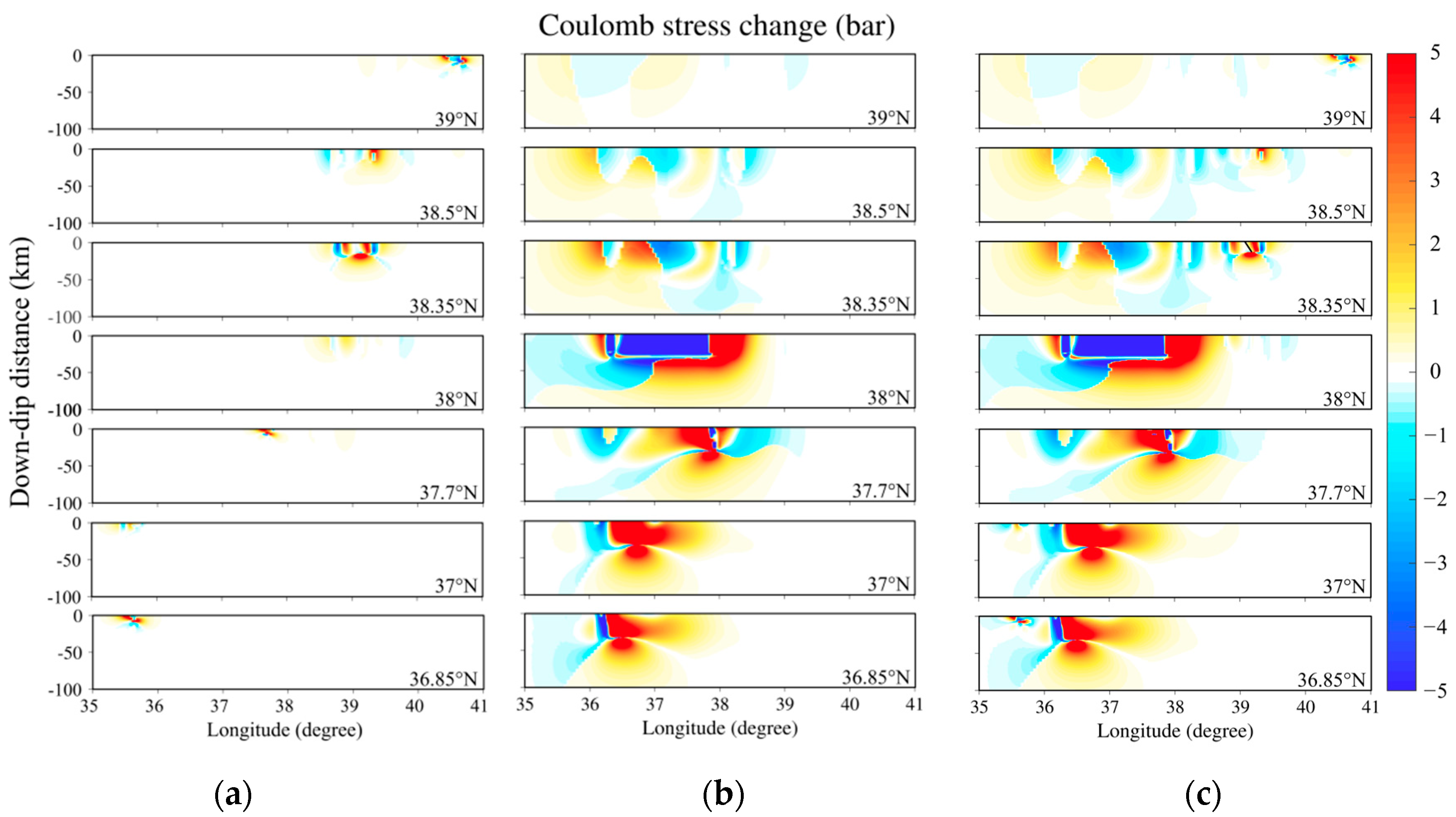
The $∆CFS$ resulting from the 7.7 Mw and 7.6 Mw earthquakes in 2023 near the East Anatolian fault zone exhibited significantly larger values and broader effects compared to several other seismic events. While the $∆CFS$ induced by three earthquakes between 1986 and 2003 only influenced the subsurface up to 10 km, the 6.8 Mw earthquake in 2020 impacted the subsurface up to 50 km. The major earthquakes in 2023 affected the subsurface up to 100 km.

(2)

Near 36.7 E, the value of $∆CFS$ is very high in the range of 37 N–36.85 N. Especially near the depth of 10–20 km, the average value reaches about 1.74–2.41 bar, which is very likely to trigger new earthquakes. In the Çardak fault zone, there is a Coulomb stress drop zone, and the drop mean value is about −2.9 bar, which significantly inhibits the continuation of earthquakes in this area.

(3)

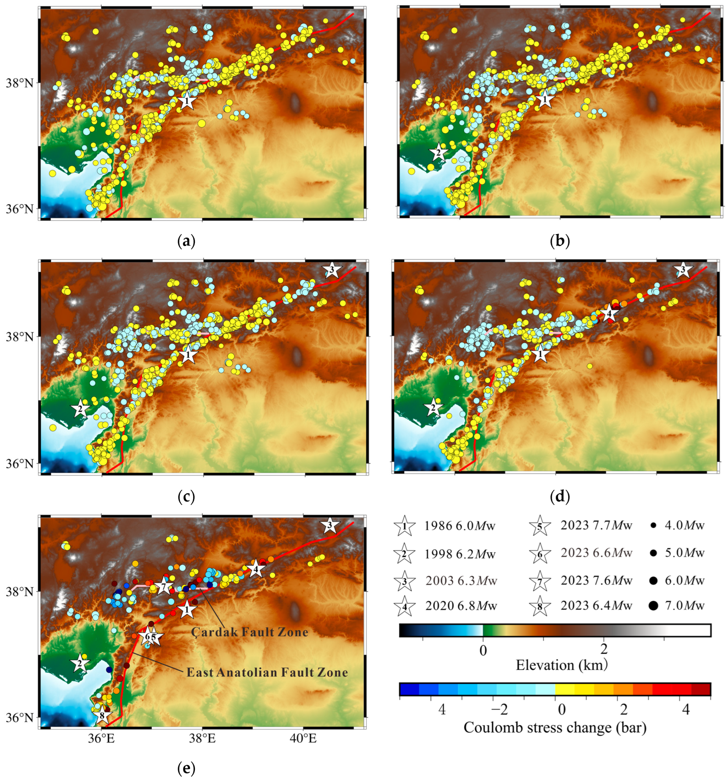
The northeastern and southwestern segments of the EAFZ have experienced Coulomb stress increases with 1.5–2.5 bar, identifying these areas as high-risk zones for future seismic activity, particularly at shallow depths (10–20 km). These areas may be accumulating strain energy, increasing the possibility of future ruptures. On the contrary, there is a 0.25–1 bar Coulomb stress drop zone in the northwest of the Çardak fault zone, where stress shadows temporarily suppress seismic activity and significantly reduce seismic risk in this region.

(4)

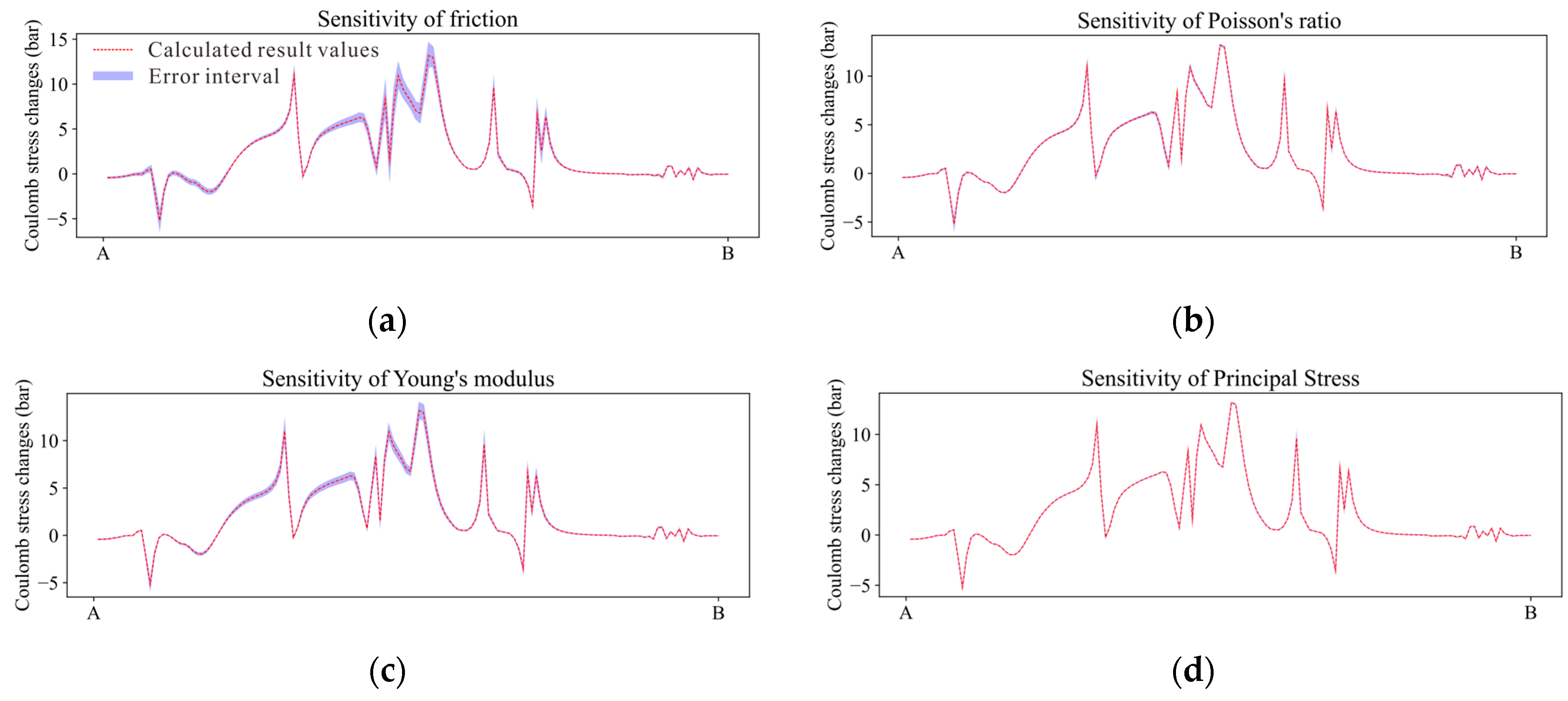
The sensitivity analysis of $∆CFS$ to various parameters revealed that the calculations were most influenced by the strike angle in the focal mechanism model, with averaging differences in results reaching up to 1.33 bar. Conversely, the direction of the principal stress axes in the study area had the least impact on Coulomb stress changes. This underscores the importance of utilizing a highly accurate focal mechanism model when conducting Coulomb stress change calculations to ensure reliable outcomes.

(5)

The three major earthquakes during 1986–2003 did not produce high $∆CFS$ for subsequent nearby earthquakes. In contrast, the five major earthquakes between 2020 and 2023 resulted in a higher $∆CFS$ for certain subsequent earthquakes in proximity. The 6.8 Mw earthquake in 2020 produced a 2-year $∆CFS$ greater than 0.1 bar on the subsequent surrounding earthquakes, which indicates that this earthquake has a promoting effect on the large earthquakes in 2023.

While this study provides valuable insights into the relationship between Coulomb stress changes and earthquake occurrence, several limitations should be acknowledged. On the one hand, the analysis is based on data from a specific time period (1986–2023) and may not fully capture the long-term behavior of Coulomb stress changes in the study region. On the other hand, the study focuses on earthquakes with magnitudes greater than 6 Mw, but the influence of smaller earthquakes on Coulomb stress changes may not have been thoroughly examined. In addition, the spatial resolution of the data and the complexity of the geological structure in the region may limit the accuracy of the Coulomb stress calculations. Future research could improve the accuracy of earthquake risk assessments from these aspects and inform more effective mitigation strategies.

References

- Li, S.; Wang, X.; Tao, T.; Zhu, Y.; Qu, X.; Li, Z.; Huang, J.; Song, S. Source Model of the 2023 Turkey Earthquake Sequence Imaged by Sentinel-1 and GPS Measurements: Implications for Heterogeneous Fault Behavior along the East Anatolian Fault Zone. Remote Sens. 2023, 15, 2618. [Google Scholar] [CrossRef]
- Mahmoud, Y.; Masson, F.; Meghraoui, M.; Cakir, Z.; Alchalbi, A.; Yavasoglu, H.; Yönlü, O.; Daoud, M.; Ergintav, S.; Inan, S. Kinematic Study at the Junction of the East Anatolian Fault and the Dead Sea Fault from GPS Measurements. J. Geodyn. 2013, 67, 30–39. [Google Scholar] [CrossRef]
- Reilinger, R.; McClusky, S.; Vernant, P.; Lawrence, S.; Ergintav, S.; Cakmak, R.; Ozener, H.; Kadirov, F.; Guliev, I.; Stepanyan, R.; et al. GPS Constraints on Continental Deformation in the Africa-Arabia-Eurasia Continental Collision Zone and Implications for the Dynamics of Plate Interactions. J. Geophys. Res. Solid Earth 2006, 111, B05411. [Google Scholar] [CrossRef]
- Yilmaz, H.; Over, S.; Ozden, S. Kinematics of the East Anatolian Fault Zone between Turkoglu (Kahramanmaras) and Celikhan (Adiyaman), Eastern Turkey. Earth Planets Space 2006, 58, 1463–1473. [Google Scholar] [CrossRef]
- Disaster and Emergency Management Authorit. 06 Şubat 2023 Pazarcık (Kahramanmaraş) Mw 7.7 ve Elbistan (Kahramanmaraş) Mw 7.6 Depremlerine Iliskin Ön Degerlendirme Raporu; Disaster and Emergency Management Authorit: Ankara, Turkey, 2023. [Google Scholar]
- Barbot, S.; Luo, H.; Wang, T.; Hamiel, Y.; Piatibratova, O.; Javed, M.T.; Braitenberg, C.; Gurbuz, G. Slip Distribution of the February 6, 2023 Mw 7.8 and Mw 7.6, Kahramanmaraş, Turkey Earthquake Sequence in the East Anatolian Fault Zone. Seismica 2023, 2. [Google Scholar] [CrossRef]
- Liu, C.; Shi, Y. Space-Time Stress Variations on the Palu-Koro Fault Impacting the 2018 Mw 7.5 Palu Earthquake and Its Seismic Hazards. Geochem. Geophys. Geosyst. 2021, 22, e2020GC009552. [Google Scholar] [CrossRef]
- Harris, R.A. Introduction to Special Section: Stress Triggers, Stress Shadows, and Implications for Seismic Hazard. J. Geophys. Res. 1998, 103, 24347–24358. [Google Scholar] [CrossRef]
- Hardebeck, J.L.; Nazareth, J.J.; Hauksson, E. The Static Stress Change Triggering Model: Constraints from Two Southern California Aftershock Sequences. J. Geophys. Res. Solid Earth 1998, 103, 24427–24437. [Google Scholar] [CrossRef]
- Gomberg, J.; Beeler, N.M.; Blanpied, M.L.; Bodin, P. Earthquake Triggering by Transient and Static Deformations. J. Geophys. Res. Solid Earth 1998, 103, 24411–24426. [Google Scholar] [CrossRef]
- Scholz, C.H. Earthquakes and Friction Laws. Nature 1998, 391, 37–42. [Google Scholar] [CrossRef]
- Rybicki, K. Analysis of Aftershocks on the Basis of Dislocation Theory. Phys. Earth Planet. Inter. 1973, 7, 409–422. [Google Scholar] [CrossRef]
- Das, S.; Scholz, C.H. Off-Fault Aftershock Clusters Caused by Shear Stress Increase? Bull. Seismol. Soc. Am. 1981, 71, 1669–1675. [Google Scholar] [CrossRef]
- Stein, R.S.; Lisowski, M. The 1979 Homestead Valley Earthquake Sequence, California: Control of Aftershocks and Postseismic Deformation. J. Geophys. Res. Solid Earth 1983, 88, 6477–6490. [Google Scholar] [CrossRef]
- Wang, M.; Liu, Z.; Luo, R. Stress Triggering Effect on the 2022 Honghe MS5.0 Earthquake with Historical Strong Earthquakes. Geod. Geodyn. 2024, 15, 107–113. [Google Scholar] [CrossRef]
- Stein, R.S.; King, G.C.P.; Lin, J. Change in Failure Stress on the Southern San Andreas Fault System Caused by the 1992 Magnitude = 7.4 Landers Earthquake. Science 1992, 258, 1328–1332. [Google Scholar] [CrossRef]
- Anderson, G.; Aagaard, B.; Hudnut, K. Fault Interactions and Large Complex Earthquakes in the Los Angeles Area. Science 2003, 302, 1946–1949. [Google Scholar] [CrossRef]
- Pollitz, F.F.; Banerjee, P.; Bürgmann, R.; Hashimoto, M.; Choosakul, N. Stress Changes along the Sunda Trench Following the 26 December 2004 Sumatra-Andaman and 28 March 2005 Nias Earthquakes. Geophys. Res. Lett. 2006, 33, L06309. [Google Scholar] [CrossRef]
- Shan, B.; Xiong, X.; Wang, R.; Zheng, Y.; Yang, S. Coulomb Stress Evolution along Xianshuihe–Xiaojiang Fault System since 1713 and Its Interaction with Wenchuan Earthquake, May 12, 2008. Earth Planet. Sci. Lett. 2013, 377–378, 199–210. [Google Scholar] [CrossRef]
- Herman, M.W.; Furlong, K.P.; Hayes, G.P.; Benz, H.M. Foreshock Triggering of the 1 April 2014 Mw 8.2 Iquique, Chile, Earthquake. Earth Planet. Sci. Lett. 2016, 447, 119–129. [Google Scholar] [CrossRef]
- Jia, Z.; Jin, Z.; Marchandon, M.; Ulrich, T.; Gabriel, A.-A.; Fan, W.; Shearer, P.; Zou, X.; Rekoske, J.; Bulut, F.; et al. The Complex Dynamics of the 2023 Kahramanmaraş, Turkey, Mw 7.8–7.7 Earthquake Doublet. Science 2023, 381, 985–990. [Google Scholar] [CrossRef]
- Liu, C.; Dong, P.; Zhu, B.; Shi, Y. Stress Shadow on the Southwest Portion of the Longmen Shan Fault Impacted the 2008 Wenchuan Earthquake Rupture. JGR Solid Earth 2018, 123, 9963–9981. [Google Scholar] [CrossRef]
- Meade, B.J.; DeVries, P.M.R.; Faller, J.; Viegas, F.; Wattenberg, M. What Is Better Than Coulomb Failure Stress? A Ranking of Scalar Static Stress Triggering Mechanisms from 105 Mainshock-Aftershock Pairs. Geophys. Res. Lett. 2017, 44, 11409–11416. [Google Scholar] [CrossRef]
- Pang, Y. Stress Evolution on Major Faults in Tien Shan and Implications for Seismic Hazard. J. Geodyn. 2022, 153–154, 101939. [Google Scholar] [CrossRef]
- Alkan, H.; Büyüksaraç, A.; BEKTAŞ, Ö. Investigation of Earthquake Sequence and Stress Transfer in the Eastern Anatolia Fault Zone by Coulomb Stress Analysis. Turk. J. Earth Sci. 2024, 33, 56–68. [Google Scholar] [CrossRef]
- Bayrak, E.; Coban, K.H. Evaluation of 08 August 2019 Bozkurt (Denizli-Turkey, Mw 6.0) Earthquake in Terms of Strong Ground-Motion Parameters and Coulomb Stress Changes. Environ. Earth Sci. 2023, 82, 470. [Google Scholar] [CrossRef]
- Kazemi, F.; Asgarkhani, N.; Jankowski, R. Machine Learning-Based Seismic Fragility and Seismic Vulnerability Assessment of Reinforced Concrete Structures. Soil Dyn. Earthq. Eng. 2023, 166, 107761. [Google Scholar] [CrossRef]
- Xu, J.; Liu, C.; Xiong, X. Source Process of the 24 January 2020 Mw 6.7 East Anatolian Fault Zone, Turkey, Earthquake. Seismol. Res. Lett. 2020, 91, 3120–3128. [Google Scholar] [CrossRef]
- Dogan, U.; Demir, D.Ö.; Çakir, Z.; Ergintav, S.; Ozener, H.; Akoğlu, A.M.; Nalbant, S.S.; Reilinger, R. Postseismic Deformation Following the Mw 7.2, 23 October 2011 Van Earthquake (Turkey): Evidence for Aseismic Fault Reactivation: October 23, 2011 Van Earthquake (Turkey). Geophys. Res. Lett. 2014, 41, 2334–2341. [Google Scholar] [CrossRef]
- Duman, T.Y.; Emre, Ö. The East Anatolian Fault: Geometry, Segmentation and Jog Characteristics. Geol. Soc. Lond. Spec. Publ. 2013, 372, 495–529. [Google Scholar] [CrossRef]
- Wollin, C.; Bohnhoff, M.; Vavryčuk, V.; Martínez-Garzón, P. Stress Inversion of Regional Seismicity in the Sea of Marmara Region, Turkey. Pure Appl. Geophys. 2019, 176, 1269–1291. [Google Scholar] [CrossRef]
- Ma, J.; Wang, P.; Vavryčuk, V.; Wu, S.; Hou, J.; Qi, Z. Tectonic Stress Field Related to the Eastern Turkey from 1976 to 2024. J. Seismol. 2025. [Google Scholar] [CrossRef]
- Ren, C.; Wang, Z.; Taymaz, T.; Hu, N.; Luo, H.; Zhao, Z.; Yue, H.; Song, X.; Shen, Z.; Xu, H.; et al. Supershear Triggering and Cascading Fault Ruptures of the 2023 Kahramanmaraş, Türkiye, Earthquake Doublet. Science 2024, 383, 305–311. [Google Scholar] [CrossRef]
- Toda, S.; Stein, R.S. The Role of Stress Transfer in Rupture Nucleation and Inhibition in the 2023 Kahramanmaraş, Türkiye, Sequence, and a One-Year Earthquake Forecast. Seismol. Res. Lett. 2024, 95, 596–606. [Google Scholar] [CrossRef]
- Tung, S.; Sippl, C.; Shirzaei, M.; Taymaz, T.; Masterlark, T.; Medved, I. Structural Controls on Fault Slip Models of the 6 February 2023 Kahramanmaraş, Türkiye Earthquake Doublet with Finite Element Analyses. Geophys. Res. Lett. 2024, 51, e2023GL107472. [Google Scholar] [CrossRef]
- Kobayashi, T.; Munekane, H.; Kuwahara, M.; Furui, H. Insights on the 2023 Kahramanmaraş Earthquake, Turkey, from InSAR: Fault Locations, Rupture Styles and Induced Deformation. Geophys. J. Int. 2024, 236, 1068–1088. [Google Scholar] [CrossRef]
- Liu, C.; Lay, T.; Wang, R.; Taymaz, T.; Xie, Z.; Xiong, X.; Irmak, T.S.; Kahraman, M.; Erman, C. Complex Multi-Fault Rupture and Triggering during the 2023 Earthquake Doublet in Southeastern Türkiye. Nat. Commun. 2023, 14, 5564. [Google Scholar] [CrossRef]
- Gallovič, F.; Zahradník, J.; Plicka, V.; Sokos, E.; Evangelidis, C.; Fountoulakis, I.; Turhan, F. Complex Rupture Dynamics on an Immature Fault during the 2020 Mw 6.8 Elazığ Earthquake, Turkey. Commun. Earth Environ. 2020, 1, 40. [Google Scholar] [CrossRef]
- Cakir, Z.; Doğan, U.; Akoğlu, A.M.; Ergintav, S.; Özarpacı, S.; Özdemir, A.; Nozadkhalil, T.; Çakir, N.; Zabcı, C.; Erkoç, M.H.; et al. Arrest of the Mw 6.8 January 24, 2020 Elaziğ (Turkey) Earthquake by Shallow Fault Creep. Earth Planet. Sci. Lett. 2023, 608, 118085. [Google Scholar] [CrossRef]
- Ding, H.; Zhou, Y.; Ge, Z.; Taymaz, T.; Ghosh, A.; Xu, H.; Irmak, T.S.; Song, X. High-Resolution Seismicity Imaging and Early Aftershock Migration of the 2023 Kahramanmaraş (SE Türkiye) MW7.9 & 7.8 Earthquake Doublet. Earthq. Sci. 2023, 36, 417–432. [Google Scholar] [CrossRef]
- Wu, F.; Xie, J.; An, Z.; Lyu, C.; Taymaz, T.; Irmak, T.S.; Li, X.; Wen, Z.; Zhou, B. Pulse-like Ground Motion Observed during the 6 February 2023 MW7.8 Pazarcık Earthquake (Kahramanmaraş, SE Türkiye). Earthq. Sci. 2023, 36, 328–339. [Google Scholar] [CrossRef]
- Zhang, Y.; Tang, X.; Liu, D.; Taymaz, T.; Eken, T.; Guo, R.; Zheng, Y.; Wang, J.; Sun, H. Geometric Controls on Cascading Rupture of the 2023 Kahramanmaraş Earthquake Doublet. Nat. Geosci. 2023, 16, 1054–1060. [Google Scholar] [CrossRef]
- Hasterok, D.; Halpin, J.A.; Collins, A.S.; Hand, M.; Kreemer, C.; Gard, M.G.; Glorie, S. New Maps of Global Geological Provinces and Tectonic Plates. Earth-Sci. Rev. 2022, 231, 104069. [Google Scholar] [CrossRef]
- Bird, P. An Updated Digital Model of Plate Boundaries. Geochem. Geophys. Grosyst. 2003, 4, 1027. [Google Scholar] [CrossRef]
- King, G.C.P.; Stein, R.S.; Lin, J. Static Stress Changes and the Triggering of Earthquakes. Bull. Seismol. Soc. Am. 1994, 84, 935–953. [Google Scholar] [CrossRef]
- Freed, A.M. Earthquake Triggering by Static, Dynamic, and Postseismic Stress Transfer. Annu. Rev. Earth Planet. Sci. 2005, 33, 335–367. [Google Scholar] [CrossRef]
- Stein, R.S. The Role of Stress Transfer in Earthquake Occurrence. Nature 1999, 402, 605–609. [Google Scholar] [CrossRef]
- Harris, R.A.; Simpson, R.W.; Reasenberg, P.A. Influence of Static Stress Changes on Earthquake Locations in Southern California. Nature 1995, 375, 221–224. [Google Scholar] [CrossRef]
- Harris, R.A.; Simpson, R.W. Suppression of Large Earthquakes by Stress Shadows: A Comparison of Coulomb and Rate-and-State Failure. J. Geophys. Res. Solid Earth 1998, 103, 24439–24451. [Google Scholar] [CrossRef]
- Okada, Y. Internal Deformation Due to Shear and Tensile Faults in a Half-Space. Bull. Seismol. Soc. Am. 1992, 82, 1018–1040. [Google Scholar] [CrossRef]
- Lin, J.; Stein, R.S. Stress Triggering in Thrust and Subduction Earthquakes and Stress Interaction between the Southern San Andreas and Nearby Thrust and Strike-Slip Faults: Stress Triggering and Fault Interaction. J. Geophys. Res. 2004, 109, B02303. [Google Scholar] [CrossRef]
- Toda, S. Forecasting the Evolution of Seismicity in Southern California: Animations Built on Earthquake Stress Transfer. J. Geophys. Res. 2005, 110, B05S16. [Google Scholar] [CrossRef]
- Gephart, J.W.; Forsyth, D.W. An Improved Method for Determining the Regional Stress Tensor Using Earthquake Focal Mechanism Data: Application to the San Fernando Earthquake Sequence. J. Geophys. Res. 1984, 89, 9305–9320. [Google Scholar] [CrossRef]
- Hardebeck, J.L.; Michael, A.J. Damped Regional-Scale Stress Inversions: Methodology and Examples for Southern California and the Coalinga Aftershock Sequence. J. Geophys. Res. Solid Earth 2006, 111, B11310. [Google Scholar] [CrossRef]
- Lund, B.; Slunga, R. Stress Tensor Inversion Using Detailed Microearthquake Information and Stability Constraints: Application to Ölfus in Southwest Iceland. J. Geophys. Res. 1999, 104, 14947–14964. [Google Scholar] [CrossRef]
- Michael, A.J. Use of Focal Mechanisms to Determine Stress: A Control Study. J. Geophys. Res. 1987, 92, 357–368. [Google Scholar] [CrossRef]
- Vavryčuk, V. Iterative Joint Inversion for Stress and Fault Orientations from Focal Mechanisms|Geophysical Journal International|Oxford Academic. Available online: https://academic.oup.com/gji/article/199/1/69/723251 (accessed on 14 October 2022).
- Bott, M.H.P. The Mechanics of Oblique Slip Faulting. Geol. Mag. 1959, 96, 109–117. [Google Scholar] [CrossRef]
- Wallace, R.E. Geometry of Shearing Stress and Relation to Faulting. J. Geol. 1951, 59, 118–130. [Google Scholar] [CrossRef]
- Michael, A.J. Determination of Stress from Slip Data: Faults and Folds. J. Geophys. Res. 1984, 89, 11517–11526. [Google Scholar] [CrossRef]
- Lentas, K. Towards Routine Determination of Focal Mechanisms Obtained from First Motion P-Wave Arrivals. Geophys. J. Int. 2018, 212, 1665–1686. [Google Scholar] [CrossRef]
- Lentas, K.; Di Giacomo, D.; Harris, J.; Storchak, D.A. The ISC Bulletin as a Comprehensive Source of Earthquake Source Mechanisms. Earth Syst. Sci. Data 2019, 11, 565–578. [Google Scholar] [CrossRef]
- Xiong, X.; Shan, B.; Zhou, Y.M.; Wei, S.J.; Li, Y.D.; Wang, R.J.; Zheng, Y. Coulomb Stress Transfer and Accumulation on the Sagaing Fault, Myanmar, over the Past 110 Years and Its Implications for Seismic Hazard. Geophys. Res. Lett. 2017, 44, 4781–4789. [Google Scholar] [CrossRef]
- Wells, D.L.; Coppersmith, K.J. New Empirical Relationships among Magnitude, Rupture Length, Rupture Width, Rupture Area, and Surface Displacement. Bull. Seismol. Soc. Am. 1994, 84, 974–1002. [Google Scholar] [CrossRef]
- Stein, R.S.; Toda, S.; Özbakir, A.D.; Sevilgen, V.; Gonzalez-Huizar, H.; Lotto, G.; Sevilgen, S. Interactions, Stress Changes, Mysteries, and Partial Forecasts of the 2023 Kahramanmaraş, Türkiye, Earthquakes. 2023. Available online: https://temblor.net/ (accessed on 12 May 2024).
- Zaccagnino, D.; Telesca, L.; Tan, O.; Doglioni, C. Clustering Analysis of Seismicity in the Anatolian Region with Implications for Seismic Hazard. Entropy 2023, 25, 835. [Google Scholar] [CrossRef] [PubMed]
- Alkan, H.; Büyüksaraç, A.; Bektaş, Ö.; Işık, E. Coulomb Stress Change before and after 24.01.2020 Sivrice (Elazığ) Earthquake (Mw = 6.8) on the East Anatolian Fault Zone. Arab. J. Geosci. 2021, 14, 2648. [Google Scholar] [CrossRef]
- Hunter, J.D. Matplotlib: A 2D Graphics Environment. Comput. Sci. Eng. 2007, 9, 90–95. [Google Scholar] [CrossRef]
- Wessel, P.; Luis, J.F.; Uieda, L.; Scharroo, R.; Wobbe, F.; Smith, W.H.F.; Tian, D. The Generic Mapping Tools Version 6. Geochem. Geophys. Geosyst. 2019, 20, 5556–5564. [Google Scholar] [CrossRef]