Abstract
The study compares the performance parameters of an Automated Guided Vehicle (AGV) equipped with optical navigation, focusing on two solutions: one utilizing reflective optocouplers and the other employing a camera. These components, commonly used in AGV optical navigation systems, differ in factors such as cost and the sophistication of control methods. The primary objective of the research was to evaluate the performance criteria of the analyzed optical navigation methods, with particular attention paid to electricity consumption, power profiles during specific transit tasks, and total transit time. The analysis also investigated two potential installation locations for the reflective optocouplers and the camera on the vehicle. The results indicate that the camera-based optical navigation method is more efficient. Specifically, the average energy consumption was approximately 26% lower when using the camera compared to the reflective optocouplers. Furthermore, the study revealed that the location of the camera had minimal influence on the vehicle’s energy consumption, whereas the location of the reflective optocouplers significantly affected energy usage.
1. Introduction
Major current global problems include high greenhouse gas emissions and the related issue of global warming [1]. This highlights the necessity of reducing emissions across all sectors of the economy. This challenge is particularly significant in the transportation sector, including intra-company transportation. Such transportation increasingly relies on Automated Guided Vehicles (AGVs). AGVs have been under development for many years and are particularly popular in warehouses and production facilities, where they have become an integral part of the production process. Their implementation not only replaces human labor in repetitive tasks that do not require significant attention but also mitigates many dangerous situations associated with human error. Research on AGVs is being conducted in numerous industrial and scientific centers. A critical factor for their effective utilization is the precision in mapping the planned travel route. Accordingly, much of the research on AGVs focuses on the appropriate selection of navigation systems. Many studies aim to optimize the control algorithms for both existing vehicles and prototype models designed for specific tasks. In many prototype AGV systems, microcontrollers and development boards, such as the Atmega 328 [2], STM 32 [3,4], Atmega 128 [5], Arduino with Atmega 2560 microcontroller [6], and Arduino Uno [7], are used for control. Depending on their intended application, various sensors are employed to operate these vehicles. Existing AGVs, which navigate along physical tracks marked by lines (e.g., inductive loops or reflective line methods) detected by inductive sensors, reflective optocouplers, or cameras [8], are now being replaced by virtual lines created from images captured by cameras [9], lidars [10], laser sensors, and other technologies.
The study in [8] explored the impact of image processing using a camera to control an AGV following a line. As is shown, vehicle control is affected by image resolution, image processing parameters, and frame rate. In [10], the authors used a single Light Detection and Ranging (LIDAR) sensor to enable proper navigation in an unfamiliar environment, avoiding obstacles even in low-light conditions. To create the virtual environment in which the vehicle operates, including for obstacle detection, neural networks are often used [11,12,13]. In [12], the authors conducted simulation analyses of AGV motion control using Physics-Informed Neural Networks (PINNs) in applying nonlinear Model Predictive Control (MPC) for AGV trajectory tracking. The results presented by the authors of this work confirmed that the analyzed model works effectively under dynamic conditions. The authors of [13] proposed a machine-learning-based approach for predictive control for autonomous vehicles. The study focused on dynamic adaptation of vision systems. The advantages and disadvantages of different AGV control methods are presented, for example, in [7]. In the case of line-of-sight methods based on the analysis of route line positions, interference with line recognition caused by various factors (changes in lighting, discontinuities, traces on the pavement identified as a traffic track, etc.) can be a significant problem. These issues are the subject of [14,15], among others. The authors of [14] analyzed the problems of vision control of an AGV moving in a working area, which were associated with uneven illumination, obscuration of the line delineating the preset traffic path, or its damage, which results in incomplete or deformed images of paths, as well as additional artifacts that introduce errors in the analyzed path line. Many solutions combine multiple navigation techniques [16,17,18,19,20], which significantly improve vehicle positioning accuracy and may also allow the vehicle to move in different environments (such as open terrain [10] and indoor spaces). In [11], a combination of line detection using infrared sensors and a camera capturing the line’s position was employed. The camera was used as a sensor in the feedback loop of a proportional–integral–derivative (PID) controller. The goal of this solution was to reduce lateral oscillations during vehicle movement. In [20], the authors used an automated vehicle localization system based on ultra-wideband technology and visual guidance. There are also solutions in which infrared sensors are replaced by cameras. Cameras not only enable line identification but also recognition of markers that can be used in vehicle control [19,21,22]. The authors of [21] investigated a method for AGV navigation using a webcam and markers in the form of four directional signals and 10 letters of the alphabet. In [22], an omnidirectional camera image stream was used for AGV navigation. Route navigation was carried out using character recognition and implemented control. Among the unconventional methods of navigation can be included the system presented in [23] with AGV motion control, using cameras to recognize the hand gestures of the human operator. A significant focus is also placed on the safety of AGV movement [24] including that related to the detection and avoidance of obstacles and collisions with other vehicles [25,26]. The authors of [25] present the results of a study of an autonomous navigation system that enables AGVs to detect and avoid obstacles based on the processing of data obtained with a front camera mounted on the vehicle. Some works are devoted to the analysis of fleet control of AGVs [27,28]. In [27], simulation studies were conducted that included costs considering the number of AGVs, AGV speed, number of tasks, scheduling interval, and path length. The authors of [28] pointed out the important role of developing a control schedule for a set of AGVs, taking into account energy consumption and rational task allocation.
The authors of [29] conducted research on the use of vision-based navigation in AGVs, which complements Global Positioning System (GPS)-based navigation. The developed vision-based navigation method was applied to a mine detection and neutralization platform [30], where vision-based navigation was used to complement other types of navigation systems, such as GPS and the inertial navigation system (INS). By using the camera, it was possible to control the vehicle in the event of a GPS signal loss. This approach resulted in satisfactory vehicle control performance under real-world conditions.
An important factor in controlling an AGV is the variable speed of the vehicle, which depends on its load. Accordingly, various solutions have been proposed, including maintaining a constant vehicle speed by employing speed and inclination sensors [5]. Another solution is to measure the drive torque of the wheels and adjust the PID controller parameters based on the vehicle’s current load. This adjustment is also important for optimizing energy consumption [18].
The application of Model Predictive Control (MPC) requires the development of a model of the controlled object; in this case, the AGV. This approach enables the determination of the AGV’s path, which can account for dynamically emerging obstacles. This capability is particularly important in factories, where the increasing number of autonomous vehicles must coexist effectively. The rise in AGV traffic not only increases the risk of collisions but also reduces operational efficiency. In the study by W. Shen and D. Wu, Path Planning of an AGV Based on Artificial Potential Field and Model Predictive Control [31], the authors highlighted the advantages and disadvantages of contemporary AGV control systems. They proposed an MPC algorithm based on an Artificial Potential Field (APF), enabling path planning, trajectory tracking, and improved system performance in real-time. An important consideration for future research would also be the energy consumption of such a control system.
Previous studies have considered travel time, localization accuracy, reproduction of the assumed route, interpretation of control signals, and interference as the main criteria for evaluating navigation. However, most of these works did not take into account the impact of the control system on energy consumption. Research to date has primarily focused on refining vehicle control algorithms, while comparatively little attention has been given to comparing the operational parameters of guided vehicles using different sensors for optical navigation. The authors’ research represents an important contribution to the study of the effectiveness of various AGV navigation systems. Unlike previously presented studies, the authors emphasized energy consumption as an additional factor in evaluating a vehicle’s navigation system, which constitutes the primary novelty of this work.
2. Materials and Methods
2.1. Technical Specification of the AGV
Optical navigation systems were tested on an AGV, the design of which (Figure 1) includes a frame supported by four self-aligning support wheels. The vehicle’s propulsion is provided by two permanent magnet direct current (DC) motors that drive wheels mounted on the vehicle’s transverse axis. Each motor is integrated with a planetary gearbox, and power is transferred to the wheels via a flexible clutch.
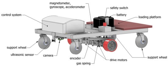
Figure 1.
Three-dimensional model of the AGV used in this study.
The project utilized a brushed DC motor with a nominal supply voltage of 12 V, manufactured by Bühler Motor (model 1.61.077.414), equipped with a gearbox featuring a gear ratio of 72.8:1. The nominal output shaft speed of the gearbox is 40 rpm, delivering a torque of 10 Ncm. The output shaft of the gearbox is connected via a flexible coupling to a shaft that is mounted in bearings within the housing of the drive system. The torque generated by this shaft is transmitted to the vehicle’s drive wheel. The other end of the motor shaft is connected via a flexible coupling to the drive shaft of an optical encoder (model MOK 30—Wobit, Pniewy, Poland); resolution: 100 ppr. The construction of the AGV’s drive system for one of the drive wheels is shown in Figure 2.
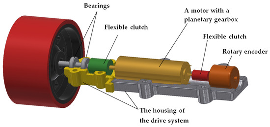
Figure 2.
Drive transmission system for one of the AGV’s drive wheels.
Control is achieved by varying the speed of the drive wheels. The drive wheels, along with the motors, are mounted on trailing arms. The vehicle is powered by a 12 V, 12 Ah AGM battery. The main dimensions of the vehicle are presented in Figure 3.
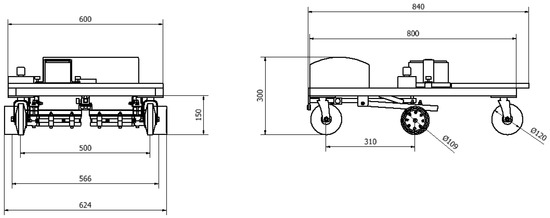
Figure 3.
Main dimensions of the AGV vehicle.
2.2. Analyzed Navigation Systems
Two optical transit identification methods for vehicle navigation have been considered, both of which use matte black tape to define the path of movement. The first solution employs two reflective transmitter–receivers mounted on a head that moves along the surface on which the vehicle is operating. This solution is shown in Figure 4. The block diagram of the control system with reflective optocouplers is presented in Figure 5.
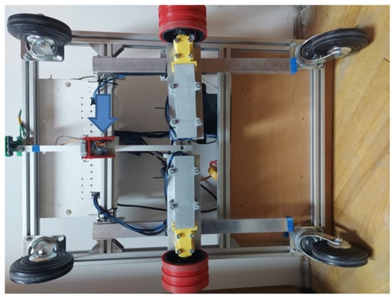
Figure 4.
The AGV with reflective optocouplers mounted (indicated by the blue arrow) on the head monitoring the position of the track tape.
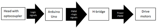
Figure 5.
Block diagram of the AGV control system with reflective optocouplers.
Two reflective optocouplers (CNY 70—VISHAY Telefunken, Wien, Austria) [32] were used for line detection. They were placed in a shared housing at a distance of 18 mm (Figure 6), ensuring a consistent distance between the reflective optocouplers and the designated line.
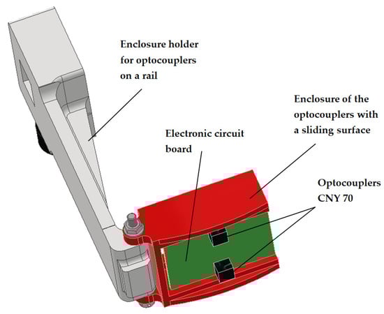
Figure 6.
Reflective optocoupler head with a mounting bracket for installation on a guide rail.
In the second solution, a camera (Figure 7) is used to determine the guiding vector based on its position relative to the tape. The block diagram of the AGV control system with a camera is presented in Figure 8.
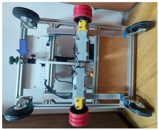
Figure 7.
The AGV with the camera mounted (indicated by blue the arrow).
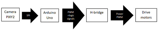
Figure 8.
Block diagram of the AGV control system with a camera.
Selected Technical Parameters of the Pixy2 Camera (SparkFun, Niwot, CO, USA) [33]:
- -
- Processor: NXP LPC4330, 204 MHz, dual-core;
- -
- Image Sensor: Aptina MT9M114, 1296 × 976 resolution with integrated image flow processor;
- -
- Lens Field-of-View: 60 degrees horizontal, 40 degrees vertical;
- -
- RAM: 264 KB;
- -
- Flash: 2 MB;
- -
- Available Data Outputs: UART serial, SPI, I2C, USB, digital, analog;
- -
- Integrated Light Source: Approximately 20 lumens;
- -
- Minimum Distance of the Camera Lens from the Object: 50 mm [34].
Both types of sensors are mounted on a bracket that allows for adjustment of the distance between the sensors and the vehicle’s drive axis (Figure 9). In both cases, the output data from the sensors is processed by an electronic control system built using an Arduino Uno module with an AtMega 328 processor running at a clock frequency of 16 MHz. The microcontroller’s output signals are transmitted to a module with an H-bridge based on the L298N chip, which controls the vehicle’s two DC motors. Each motor is controlled separately using a PWM signal (responsible for motor power) and two logic signals, which enable reversing the motor’s direction and braking. The control system allows for changes in wheel rotation direction, significantly enhancing the vehicle’s maneuverability.
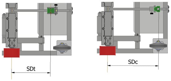
Figure 9.
The distances of the transceiver mounts (SDt) and the camera (SDc) from the vehicle’s drive axis in the horizontal plane.
Table 1 presents the settings of the Pixy2 camera used in the conducted research.

Table 1.
Camera settings in PixyMon v2 version 3.0.24 software.
2.3. Control Algorithms
During testing, the Pixy2 camera followed a designated travel route using a Line Tracking program. The line was converted into a vector, and the alignment of this vector with the screen’s axis of symmetry (Figure 10a) indicated that the vehicle’s direction was correctly aligned with the designated route. Consequently, the vehicle achieved full forward speed. When a discrepancy occurred between the designated travel route and the vehicle’s direction, the vector deviated from the screen’s axis of symmetry (Figure 10b). The parameters presented in Table 1 were selected based on extensive trials. The most influential parameters for vehicle control include camera brightness, which must be adjusted according to the intensity of the lighting. Maximum line width and minimum line width are critical for detecting the line along which the vehicle moves. If the line width is set too narrow, darker areas on the surface may be detected as a guiding line, disrupting the vehicle’s movement. Conversely, if the line width is set too wide, the line may not be detected, causing the vehicle to lose navigation. The minimum line length parameter was adjusted to ensure that the detected guiding vector extends across the entire field of view of the camera. If the value is set too low, this can cause significant disruptions in determining the vehicle’s direction vector.
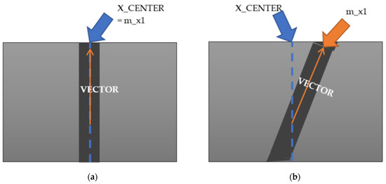
Figure 10.
Vector when the direction of the AGV aligns (a) and does not align (b) with the direction of the designated route of travel.
The vector’s coordinates can be used to calculate its deviation from the screen axis. Based on this, the error, as presented in Formula (1), is calculated following the procedure outlined in the software available on the manufacturer’s website [35]. Depending on the direction of the vector’s deviation, the error can take either positive or negative values.
where:
- m_x1—the x-coordinate of the end of the vector;
- X_CENTER—the x-coordinate of the screen center.
Based on the error information, the duty cycle of the PWM signal (0–400) is calculated using Equation (2):
where:
- error—error according to the Equation (1).
As seen in Equation (2), the speed decreases to a minimum value before starting to increase again. Once the minimum of the function is reached, the direction of the wheel’s rotation is reversed.
In optocoupler-based control (Figure 11), the time during which the reflective optocoupler does not reflect light (i.e., when it is above the black line) is measured. The accumulation of time (successive values corresponding to a certain duration) begins when the AGV moves off the route marked by the line (with the reflective optocoupler above the black line). The longer the reflective optocoupler stays in this position, the greater the accumulated time. The accumulation stops when the reflective optocoupler moves outside the black line, at which point the accrued time starts to decrease. Based on the value of this time, the control signal for the corresponding wheel is calculated using Formula (3):
where:
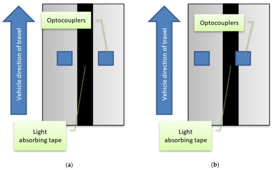
Figure 11.
The alignment of the reflective optocouplers with respect to the designated route when (a) is consistent and (b) is inconsistent with the assumed direction of the vehicle’s movement along the designated route.
- PWM—filling of the speed control signal (0–255);
- counter—the quantized value of time.
When the minimum PWM value is reached, the direction of wheel rotation is reversed.
The diagrams of the measurement system utilizing the camera are shown in Figure 12. Figure 13 presents the diagram of the measurement system utilizing a head with reflective optocouplers.
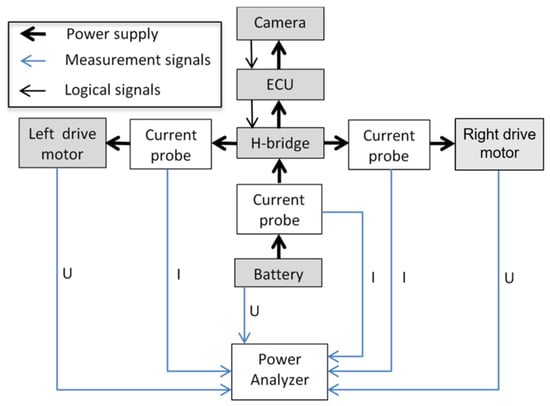
Figure 12.
Diagram of the measurement system utilizing the camera.
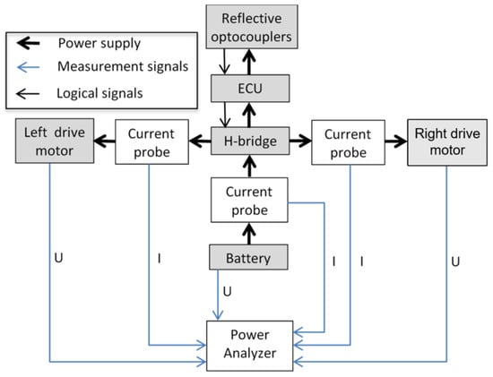
Figure 13.
Diagram of the measurement system utilizing a head with reflective optocouplers.
The diagram of the control system utilizing reflective optocouplers is shown in Figure 14, while the diagram utilizing the camera is shown in Figure 15.
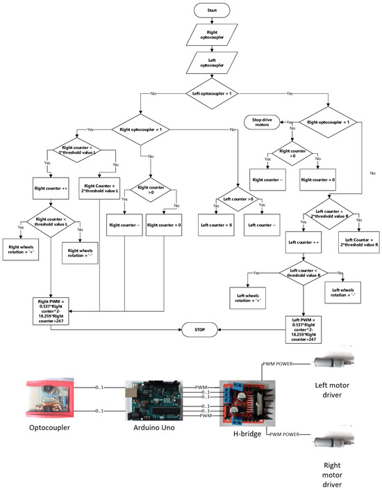
Figure 14.
The information flow diagram (upper figure) and the simplified block diagram (lower figure) of the control system utilizing reflective optocouplers.
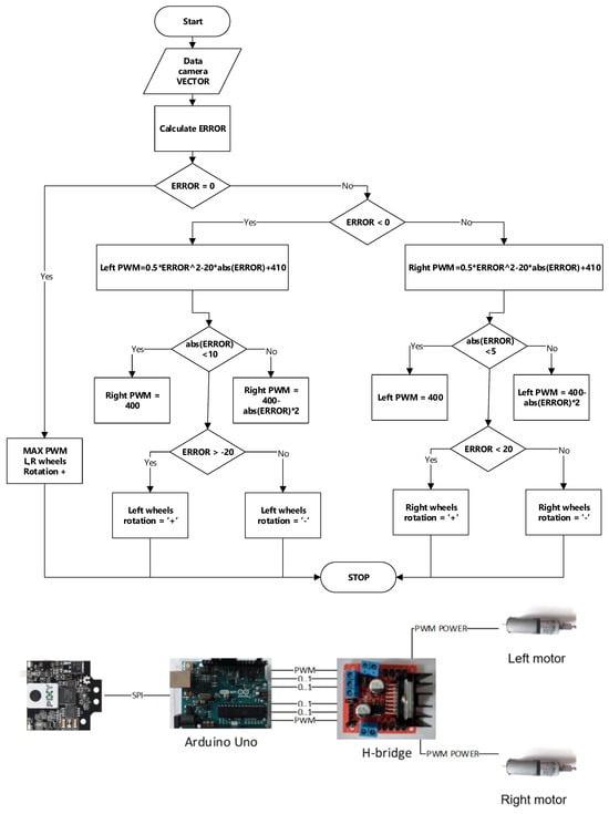
Figure 15.
The information flow diagram (upper figure) and the simplified block diagram (lower figure) of the control system utilizing the camera.
2.4. Research Procedure
Power and energy consumption measurements were carried out using the HIOKI PW 3390 power analyzer [36], equipped with three HIOKI CT6843A current probes. The power analyzer was powered by an additional 12 V 62 Ah battery via a WHITENERGY 800 W inverter. The total weight of the tested vehicle was 38.3 kg.
The power analyzer and current probes used were characterized by the measurement accuracy outlined in Table 2. The relative error in the measurement of maximum power was ±4%.
Table 2.
Power measurement accuracy.
The vehicle moved within a room along a specified path measuring 16.0 m in length, as shown in Figure 16.
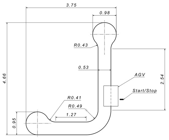
Figure 16.
Dimensions of the movement path.
The tests were conducted in a laboratory at an ambient temperature of 25 ± 3 °C.
Current measurements were taken simultaneously on the wires powering the entire vehicle (control system along with the drive system) and the wires powering both motors. Additionally, the voltage on the battery and both motors was measured using the power analyzer. These parameters were recorded at a frequency of 10 Hz.
For each sensor, two distances (250 mm and 350 mm) from the vehicle’s drive axis with the drive wheels were considered (Figure 9). The distance of the reflective optocouplers from the vehicle’s drive axis in the horizontal plane is referred to as SDt (Sensor Distance transceiver), while the distance of the camera lens from the vehicle’s drive axis is referred to as SDc (Sensor Distance camera).
First, tests were conducted on the vehicle equipped with reflective optocouplers. The vehicle was placed on the transit path as shown in Figure 16. Then, the measured parameters were registered in the power analyzer, and the drive system was activated. For each distance SDt, three measurements were performed. Based on these, the average values of selected parameters were calculated, and analyses of instantaneous power and energy consumption were carried out.
In the second phase, a camera was installed on the vehicle. Similarly, for each value of SDc, three passes were carried out. The subsequent course of the tests was identical to that of the vehicle equipped with reflective optocouplers.
3. Results and Discussion
The results of the tests are presented in Figure 17, Figure 18, Figure 19, Figure 20, Figure 21, Figure 22, Figure 23 and Figure 24. Figure 17a, Figure 18a, Figure 19a, Figure 20a, Figure 21a, Figure 22a, Figure 23a, Figure 24a show the results from the tests using reflective optocouplers, while Figure 17b, Figure 18b, Figure 19b, Figure 20b, Figure 21b, Figure 22b, Figure 23b, Figure 24b present the results from the tests using the camera.
Figure 17a shows the electrical power profile during the vehicle’s path traversal for the right wheel, using reflective optocouplers with SDt = 250 mm, while Figure 17b shows the profile using a camera with SDc = 250 mm.
There are significant differences in the power value profiles depending on the sensor used. For reflective optocouplers, the output signal of which is binary, the control system’s response to the input signal depended on the duration of the input. In contrast, with the camera, the trajectory information was transmitted as a digital signal, with its value proportional to the deviation from the target path. This resulted in greater dynamics in the changes of motor power values for the control version using reflective optocouplers.
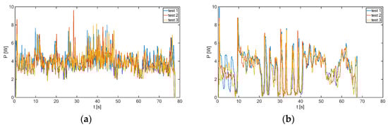
Figure 17.
The electrical power profile of the right wheel motor driving the vehicle: (a) SDt = 250 mm, (b) SDc = 250 mm.
Figure 18a shows the electrical power profile during the vehicle’s path traversal for the left wheel, using reflective optocouplers with SDt = 250 mm, while Figure 18b shows the profile using a camera with SDc = 250 mm.
As in Figure 17, the use of reflective optocouplers was associated with greater dynamics in the changes of the power value of the motor driving the left wheel.
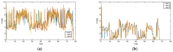
Figure 18.
The electrical power profile of the left wheel motor driving the vehicle: (a) SDt = 250 mm, (b) SDc = 250 mm.
The comparison of the power drawn from the vehicle’s battery for SDt = SDc = 250 mm is presented in Figure 19.
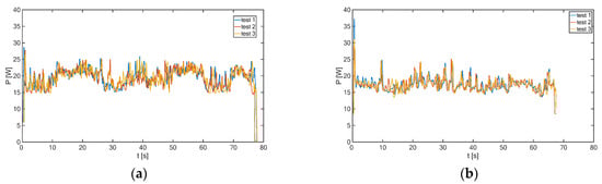
Figure 19.
The comparison of the electrical power profiles drawn from the vehicle’s battery: (a) SDt = 250 mm, (b) SDc = 250 mm.
In the case of vehicle control using a camera, higher power consumption is observed when the vehicle starts from a standstill compared to using reflective optocouplers. This is due to the ability to utilize the full power of the motors, as the control system has complete information about the position of the line defining the desired path. In contrast, for reflective optocouplers, line detection occurs “point by point”, meaning the initial acceleration values of the vehicle—and the associated power consumption by the drive motors—are lower. There are also differences in the power consumed by the AGV after stopping at the end of the transit. When using a camera, the vehicle consumes approximately 10 W after stopping, which is related to powering the control system. In contrast, when using reflective optocouplers, the vehicle’s power supply is turned off after stopping.
Figure 20a shows the electrical power profile during the vehicle’s path traversal for the right wheel using reflective optocouplers with SDt = 350 mm, while Figure 20b shows the profile using a camera with SDc = 350 mm. When using reflective optocouplers, the transit time for the desired path was noticeably longer compared to using a camera. This difference was due to the control method, which, in this case, was associated with a significantly higher frequency of the system’s response to line detection defining the desired path. Control using the camera is continuous, allowing for a proportional response of the motors to the vehicle’s deviation from the target path. The discrepancy in transit time was greater than that observed for SDt = SDc = 250 mm.
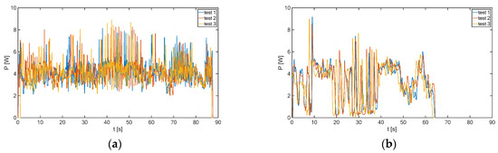
Figure 20.
The electrical power profile of the right wheel motor driving the vehicle: (a) SDt = 350 mm, (b) SDc = 350 mm.
Figure 21a shows the electrical power profile during the vehicle’s path traversal for the left wheel, using reflective optocouplers with SDt = 350 mm, while Figure 21b shows the profile using a camera with SDc = 350 mm. Similarly to the right wheel, these results confirm the advantage of using a camera for vehicle control compared to reflective optocouplers.
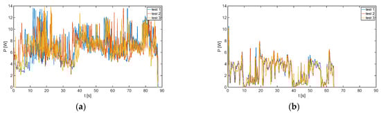
Figure 21.
The electrical power profile of the left wheel motor driving the vehicle: (a) SDt = 350 mm, (b) SDc = 350 mm.
The comparison of the power consumption from the vehicle’s battery for SDt = SDc = 350 mm is presented in Figure 22. Similarly to SDt = SDc = 250 mm, when using the camera, the transit time was noticeably shorter. The instantaneous power values drawn from the battery showed a larger range of variation and higher frequency in the configuration with reflective optocouplers.
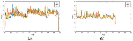
Figure 22.
The comparison of the electrical power profiles drawn from the vehicle’s battery: (a) SDt = 350 mm, (b) SDc = 350 mm.
Figure 23 presents a comparison of the power profiles for the analyzed values of SDt and SDc. Comparing the power curves in Figure 23a, it can be observed that the power registration for the distance SDt = 250 mm ended earlier, indicating a shorter transit time (by approximately 9.4 s) compared to SDt = 350 mm. This was caused by significantly higher frequencies of power oscillations. The power oscillations in the control system with reflective optocouplers are reflected in the vehicle’s oscillations during maneuvers. As mentioned, this could be due to the relatively long response time of the system to the input signal. This issue is much less pronounced in the camera-based control system, which can be explained by the presence of a processor in the Pixy camera that determines the direction of the guiding line, thereby significantly offloading the microcontroller on the Arduino Uno board. Comparing the curves in Figure 23b, it is noticeable that the transit was completed in a shorter time (about 3.3 s) with SDc = 350 mm.
With the increased transit time, there is also a noticeable increase in the vehicle’s energy consumption, as illustrated in Figure 24. When using reflective optocouplers, the placement of the optocouplers has a significant impact on average energy consumption. A larger value of SDt (350 mm) resulted in higher energy consumption and a longer transit time. This could be attributed to the control method, which, in this case, was associated with a significantly higher frequency of the system’s response to line detection defining the desired path. The transit times, energy consumption values, and average vehicle speeds are presented in Table 3.
Table 3.
Energy consumption, transit time, and speed of the AGV in the analyzed configurations (the values in the table represent averages from three measurements; the span of the measurement results is shown in parentheses).
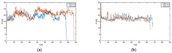
Figure 23.
Comparison of the power profiles drawn from the battery: (a) SDt = 250 mm and 350 mm, (b) SDc = 250 mm and 350 mm.
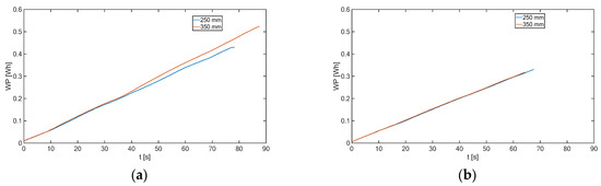
Figure 24.
Comparison of the cumulative electrical energy drawn from the battery: (a) SDt = 250 mm and 350 mm, (b) SDc = 250 mm and 350 mm.
The energy consumption values obtained using reflective optocouplers for a distance of SDt = 250 mm in consecutive tests were 0.430 Wh, 0.425 Wh, and 0.432 Wh, while for a distance of SDt = 350 mm, these values were higher, at 0.523 Wh, 0.533 Wh, and 0.515 Wh. The average energy consumption using reflective optocouplers at SDt = 350 mm was approximately 22% higher.
For the camera system, the greater distance of SDc = 350 mm was more favorable in terms of energy consumption. In the individual tests, the energy consumption for this distance was 0.317 Wh, 0.319 Wh, and 0.317 Wh. For the distance of SDc = 250 mm, the energy consumption values in the individual tests were 0.331 Wh, 0.329 Wh, and 0.329 Wh. The difference in average energy consumption using the camera for the analyzed SDc distances was approximately 4%.
The results summarized in Table 3 confirm the benefits of using a camera for the vehicle navigation system. The average energy consumption was approximately 26% lower when using the camera compared to the value obtained with reflective optocouplers. The shortest average transit time was 64.2 s (using the camera), while the longest was 87.5 s. This was also related to the higher average vehicle speeds when using the camera, which were 0.24 m/s for SDc = 250 mm and 0.25 m/s for SDc = 350 mm. In the case of using reflective optocouplers, the average speeds were 0.21 m/s for SDt = 250 mm and 0.18 m/s for SDt = 350 mm.
4. Conclusions
Based on the conducted studies, the following conclusions were formulated:
- -
- The use of camera-based control allows for a reduction in transit time and lower energy consumption by the vehicle compared to a vehicle equipped with reflective optocouplers.
- -
- The use of reflective optocouplers was associated with a greater dynamics of changes in the power values of the drive motors.
- -
- The placement of the sensors affects operational parameters, such as energy consumption and transit time. These values were lower when using the camera for SDc = 350 mm, while for reflective optocouplers, lower values were achieved for SDt = 250 mm.
- -
- The smaller dynamics of changes in the vehicle’s direction of motion (smaller transverse oscillations) when using the camera resulted in lower energy consumption.
The tested vehicle, equipped with reflective optocouplers, was previously tested under lighting conditions with varying intensities. Due to the anticipated potential impact of LED lighting (infrared light) on the photodetectors of the reflective optocouplers, lamps with this type of light source were used. The high-power lamps allowed for adjustments in light intensity and illuminated the path along which the vehicle moved. Preliminary tests showed that the light intensity from the LED lamps did not significantly affect the vehicle’s navigation capabilities when using the reflective optocouplers.
In the case of navigation using a camera, a significant influence of the room’s lighting on the ability to determine the direction vector was observed. The camera is equipped with its own light source that illuminates its “field of view”. If this light source is not used, it is necessary to adjust the “Camera brightness” depending on the ambient lighting. The camera software used in the tests was not equipped with a function for automatic brightness adjustment based on the intensity of external lighting.
However, by using the built-in camera lighting, it is possible to adjust the settings as shown in Table 1, ensuring correct path detection under drastically different room lighting conditions.
Future work includes the development of a lighting adjustment system that adapts to environmental conditions due to the “blinding effect” on the camera when the surface reflects light well. It is also planned to support vehicle navigation using codes placed along the vehicle’s route, which can be detected by the camera.
The conducted research indicates a clear difference in the operational parameters of the AGV depending on the optical navigation method used. The results can be applied when selecting the control method for an AGV, particularly with regard to energy consumption. For AGVs using optical reflective optocouplers, replacing them with camera-based navigation systems may result in reduced energy consumption and improved control of vehicle movement. These findings may also aid in optimizing AGV control algorithms and serve as a foundation for further research in this area.
Author Contributions
Conceptualization, M.J., A.J., H.K. and K.B.; methodology, M.J. and K.B.; software, K.B.; validation, M.J., A.J., H.K. and K.B.; formal analysis, M.J., A.J., H.K. and K.B.; investigation, M.J. and K.B.; resources, M.J., A.J., H.K. and K.B.; data curation, K.B.; writing—original draft preparation, M.J., A.J., H.K. and K.B.; writing—review and editing, M.J., A.J., H.K. and K.B.; visualization, K.B.; supervision, K.B. All authors have read and agreed to the published version of the manuscript.
Funding
This research received no external funding.
Institutional Review Board Statement
Not applicable.
Informed Consent Statement
Not applicable.
Data Availability Statement
The original contributions presented in the study are included in the article, further inquiries can be directed to the corresponding author.
Acknowledgments
The authors wish to acknowledge the Polish Ministry of Education and Science and the Rzeszow University of Technology for supporting this research.
Conflicts of Interest
The authors declare no conflicts of interest.
References
- IPCC. Global Warming of 1.5 °C. An IPCC Special Report on the Impacts of Global Warming of 1.5 °C Above Pre-Industrial Levels and Related Global Greenhouse Gas Emission Pathways, in the Context of Strengthening the Global Response to the Threat of Climate Change, Sustainable Development, and Efforts to Eradicate Poverty; Masson-Delmotte, V., Zhai, P., Pörtner, H.-O., Roberts, D., Skea, J., Shukla, P.R., Pirani, A., Moufouma-Okia, W., Péan, C., Pidcock, R., et al., Eds.; Cambridge University Press: Cambridge, UK; New York, NY, USA, 2018; 616p. [Google Scholar] [CrossRef]
- Sankari, J.; Imtiaz, R. Automated guided vehicle(AGV) for industrial sector. In Proceedings of the 2016 10th International Conference on Intelligent Systems and Control (ISCO), Coimbatore, India, 7–8 January 2016; pp. 1–5. [Google Scholar] [CrossRef]
- Han, Z. Research on logistics AGV vehicle path planning based on improved Q-learning algorithm. In Proceedings of the 2022 7th International Conference on Automation, Control and Robotics Engineering (CACRE), Xi’an, China, 14–16 July 2022; pp. 264–268. [Google Scholar] [CrossRef]
- Bi, X.; He, Q.; Li, Y.; Liu, G.; Li, X. AGV magnetic navigation unmanned vehicle handling wood automation. In Proceedings of the Third International Conference on Control and Intelligent Robotics (ICCIR 2023), Sipsongpanna, China, 30 June–2 July 2023; Volume 12940, p. 129400A. [Google Scholar] [CrossRef]
- Silvirianti, A.; Krisna, A.S.R.; Rusdinar, A.; Yuwono, S.; Nugraha, R. Speed control system design using fuzzy-PID for load variation of automated guided vehicle (AGV). In Proceedings of the 2017 2nd International Conference on Frontiers of Sensors Technologies (ICFST), Shenzhen, China, 14–16 April 2017; pp. 426–430. [Google Scholar] [CrossRef]
- Apsada, S.; Risfendra, R. Improving the Accuracy of Manual Control of an Automatic Guided Vehicle (AGV) Robot by Applying the Proportional Integral Derivative (PID) Algorithm. JTEIN J. Tek. Elektro Indones. 2024, 5, 343–354. [Google Scholar] [CrossRef]
- Baballe, M.A.; Adamu, A.I.; Bari, A.S.; Ibrahim, A. Principle Operation of a Line Follower Robot. J. Math. Tech. Comput. Math. 2023, 2, 211–215. [Google Scholar]
- Puppim de Oliveira, D.; Pereira Neves dos Reis, W.; Morandin Junior, O. A Qualitative Analysis of a USB Camera for AGV Control. Sensors 2019, 19, 4111. [Google Scholar] [CrossRef] [PubMed]
- Zheng, Z.; Lu, Y. Research on AGV trackless guidance technology based on the global vision. Sci. Prog. 2022, 105, 00368504221103766. [Google Scholar] [CrossRef]
- Baras, N.; Nantzios, G.; Ziouzios, D.; Dasygenis, M. Autonomous Obstacle Avoidance Vehicle Using LIDAR and an Embedded System. In Proceedings of the 2019 8th International Conference on Modern Circuits and Systems Technologies (MOCAST), Thessaloniki, Greece, 13–15 May 2019. [Google Scholar]
- Varagul, J.; Ito, T. Simulation of Detecting Function object for AGV Using Computer Vision with Neural Network. Procedia Comput. Sci. 2016, 96, 159–168. [Google Scholar] [CrossRef]
- Li, Y.; Liu, L. Physics-Informed Neural Network-Based Nonlinear Model Predictive Control for Automated Guided Vehicle Trajectory Tracking. World Electr. Veh. J. 2024, 15, 460. [Google Scholar] [CrossRef]
- Grigorescu, S.; Ginerica, C.; Zaha, M.; Macesanu, G.; Trasnea, B. LVD-NMPC: A learning-based vision dynamics approach to nonlinear model predictive control for autonomous vehicles. Int. J. Adv. Robot. Syst. 2021, 18. [Google Scholar] [CrossRef]
- Wu, X.; Sun, C.; Zou, T.; Xiao, H.; Wang, L.; Zhai, J. Intelligent Path Recognition against Image Noises for Vision Guidance of Automated Guided Vehicles in a Complex Workspace. Appl. Sci. 2019, 9, 4108. [Google Scholar] [CrossRef]
- Zhang, H.; Xu, L.; Liang, J.; Sun, X. Research on Guide Line Identification and Lateral Motion Control of AGV in Complex Environments. Machines 2022, 10, 121. [Google Scholar] [CrossRef]
- Kim, S.H.; Park, K.S. A Study on Navigation Sensor System for Outdoor AGV Using AMR Sensors. J. Control Autom. Syst. Eng. 2003, 9, 140–146. [Google Scholar] [CrossRef]
- Manikandan, S.; Kaliyaperumal, G.; Hakak, S.; Gadekallu, T.R. Curve-Aware Model Predictive Control (C-MPC) Trajectory Tracking for Automated Guided Vehicle (AGV) over On-Road, In-Door, and Agricultural-Land. Sustainability 2022, 14, 12021. [Google Scholar] [CrossRef]
- Yang, X.; Hu, H.; Cheng, C.; Wang, Y. Automated Guided Vehicle (AGV) Scheduling in Automated Container Terminals (ACTs) Focusing on Battery Swapping and Speed Control. J. Mar. Sci. Eng. 2023, 11, 1852. [Google Scholar] [CrossRef]
- Jang, J.-Y.; Yoon, S.-J.; Lin, C.-H. Automated Guided Vehicle (AGV) Driving System Using Vision Sensor and Color Code. Electronics 2023, 12, 1415. [Google Scholar] [CrossRef]
- Hu, X.; Luo, Z.; Jiang, W. AGV Localization System Based on Ultra-Wideband and Vision Guidance. Electronics 2020, 9, 448. [Google Scholar] [CrossRef]
- Lee, J.; Hyun, C.-H.; Park, M. A Vision-Based Automated Guided Vehicle System with Marker Recognition for Indoor Use. Sensors 2013, 13, 10052–10073. [Google Scholar] [CrossRef]
- Kotze, B.; Jordaan, G. Investigation of Matlab® as Platform in Navigation and Control of an Automatic Guided Vehicle Utilising an Omnivision Sensor. Sensors 2014, 14, 15669–15686. [Google Scholar] [CrossRef] [PubMed]
- Budzan, S.; Wyżgolik, R.; Kciuk, M.; Kulik, K.; Masłowski, R.; Ptasiński, W.; Szkurłat, O.; Szwedka, M.; Woźniak, Ł. Using Gesture Recognition for AGV Control: Preliminary Research. Sensors 2023, 23, 3109. [Google Scholar] [CrossRef]
- Ho, Y.-C.; Liao, T.-W. Zone design and control for vehicle collision prevention and load balancing in a zone control AGV system. Comput. Ind. Eng. 2009, 56, 417–432. [Google Scholar] [CrossRef]
- Pires, M.; Couto, P.; Santos, A.; Filipe, V. Obstacle Detection for Autonomous Guided Vehicles through Point Cloud Clustering Using Depth Data. Machines 2022, 10, 332. [Google Scholar] [CrossRef]
- Li, Q.; Pogromsky, A.; Adriaansen, T.; Udding, J.T. A Control of Collision and Deadlock Avoidance for Automated Guided Vehicles with a Fault-Tolerance Capability. Int. J. Adv. Robot. Syst. 2016, 13, 64. [Google Scholar] [CrossRef]
- Zhang, T.; Xu, M.; Ma, Z.; Ma, F.; Yu, L. A scheduling optimization method for multiple automated guided vehicle systems. Int. J. Adv. Robot. Syst. 2024, 21, 17298806241246888. [Google Scholar] [CrossRef]
- Wang, F.; Zhang, Y.; Su, Z. A novel scheduling method for automated guided vehicles in workshop environments. Int. J. Adv. Robot. Syst. 2019, 16, 1729881419844152. [Google Scholar] [CrossRef]
- Głębocki, R.; Zasuwa, M.; Świętoń, G. Visual navigation for autonomous land vehicle. Pomiary Autom. Robot. 2010, 2, 45–50. [Google Scholar]
- Głębocki, R.; Świętoń, G. Some aspects of control and navigation system for autonomous UGV. Pomiary Autom. Robot. 2011, 2, 23–30. [Google Scholar]
- Shen, W.; Wu, D. Path planning of an AGV based on artificial potential field and model predictive control. In Proceedings of the 2021 33rd Chinese Control and Decision Conference (CCDC), Kunming, China, 22–24 May 2021; pp. 6925–6930. [Google Scholar] [CrossRef]
- Reflective Optical Sensor with Transistor Output. Available online: https://www.vishay.com/docs/83751/cny70.pdf (accessed on 17 January 2025).
- Pixy 2 CMUcam5 Smart Vision Sensor. Available online: https://media.digikey.com/pdf/Data%20Sheets/Seeed%20Technology/102991074_Web.pdf (accessed on 19 January 2025).
- PIXY Documentation. Available online: https://docs.pixycam.com/wiki/doku.php?id=wiki:v2:what_is_the_maximum_distance_that_pixy_can_detect_objects (accessed on 16 January 2025).
- PIXY Documentation. Available online: https://pixycam.com/downloads-pixy1/ (accessed on 4 May 2024).
- Hioki. Power Meters/Power Analyzer. Available online: https://www.hioki.com/euro-en/products/power-meters/power-analyzer/id_5964 (accessed on 4 May 2024).
Disclaimer/Publisher’s Note: The statements, opinions and data contained in all publications are solely those of the individual author(s) and contributor(s) and not of MDPI and/or the editor(s). MDPI and/or the editor(s) disclaim responsibility for any injury to people or property resulting from any ideas, methods, instructions or products referred to in the content. |
© 2025 by the authors. Licensee MDPI, Basel, Switzerland. This article is an open access article distributed under the terms and conditions of the Creative Commons Attribution (CC BY) license (https://creativecommons.org/licenses/by/4.0/).