A Multi-Time Scale Hierarchical Coordinated Optimization Operation Strategy for Distribution Networks with Aggregated Distributed Energy Storage

Abstract

In recent years, with the steady growth of load demand in distribution networks, the fluctuation and uncertainty of power loads have significantly increased. Meanwhile, the rising penetration of photovoltaic generation has further exacerbated the challenges of power system accommodation capability. To enhance photovoltaic accommodation capability and realize the secure and economic operation of distribution networks, a multi-time scale hierarchical coordinated optimization operation strategy for distribution networks with aggregated distributed energy storage has been proposed. First, the regulation requirements of aggregated distributed energy storage are analyzed, and a distributed energy storage aggregation model is established based on an inner approximate Minkowski Sum. Subsequently, a multi-time scale optimization operation model considering source-load uncertainties for day-ahead, intra-day, and real-time stages is developed based on a stepped carbon emission cost model. Then, a power allocation method within the aggregated distributed energy storage based on the water-filling algorithm is presented. Finally, a practical distribution network in a demonstration county in China is used as a case study to validate the proposed method. The results demonstrate that the proposed strategy effectively reduces system operation costs while improving photovoltaic accommodation capacity and enhancing the reliability of system operation.

1. Introduction

With the steady growth of peak load demand in recent years and the large-scale deployment of intermittent renewable energy resources, the fluctuation levels and uncertainties of power loads have significantly increased [1,2]. Moreover, the increasing integration of distributed photovoltaic (PV) systems into distribution networks (DNs) has overwhelmed the power system’s accommodation capability, resulting in resource waste such as PV curtailment [3]. Under such circumstances, relying on traditional regulation methods has proven insufficient to ensure the secure, stable, and economical operation of power systems [4]. On the other hand, abundant distributed energy storage (DES) resources within DNs can be utilized to provide flexible regulation services, helping to alleviate the pressure on power grids caused by the integration of renewable energy generation and rapid load growth [5,6,7]. Compared with traditional centralized energy storage stations, DES has advantages such as a smaller footprint and lower investment costs, allowing it to be flexibly installed at various locations on the user side [8]. However, the small power and limited capacity of individual DES systems make them unsuitable for direct participation in grid regulation, leading to their regulation potential being underutilized [9]. In contrast, aggregated DES clusters offer greater flexibility and controllable potential for regulation [10]. Therefore, it is necessary to manage DES aggregation, enabling it to participate as a controllable resource in the optimal operation of DNs.

The aggregation of feasible regions for DES refers to the process where the wide-area DES resources are aggregated into an overall feasible region, based on the satisfaction of each individual resource’s feasible region, through certain aggregation methods. These resources are then managed and scheduled in a unified manner [11]. The feasible region aggregation is mathematically represented as the addition operation in Euclidean space [12], specifically the Minkowski Sum. However, the computation of the Minkowski Sum for two arbitrary polygons is categorized as a nondeterministic polynomial (NP) problem, for which no efficient solution algorithm currently exists [13]. As a result, many studies have focused on developing approximate feasible domain models with specific rules to simplify the aggregation process. In Ref. [14], convex polyhedra were used to describe the feasible regions of resources, and an approximate method was proposed to simplify the feasible region aggregation of energy storage. In Ref. [15], an inner-approximation approach integrating constrained spaces was adopted, where the constraint spaces of all individuals within the cluster were integrated before participating in power system operations. In Ref. [16], a mathematical model of the exact aggregated feasible region for distributed resources was derived, and a k -order approximation model was used to compute a high-accuracy enclosing model for the feasible region aggregation. In Ref. [17], high-dimensional ellipsoids were employed to approximate the feasible regions of distributed resources, ensuring the aggregation optimality and decomposition feasibility. However, outer-approximation methods among these studies may lead to infeasibility during practical scheduling, while inner-approximation methods often sacrifice significant resource flexibility.

In the context of energy storage systems (ESS) participating in the optimal operation of DNs, a resilient microgrid energy management model, which includes diesel generators, energy storage, and load scheduling, is constructed in Ref. [18], and a multi-stage constraint-handling multi-objective optimization method tailored for resilient microgrid energy management is proposed. In Ref. [19], a day-ahead scheduling plan was formulated by integrating the multi-time scale characteristics of ESS and various demand response resources on the load side. High prediction accuracy was achieved through intra-day rolling scheduling and real-time adjustments. In Ref. [20], a hidden layer-based attack-resilient distributed cooperative control algorithm was introduced for the secondary control of islanded microgrids. In Ref. [21], to address the intermittency of renewable energy generation, the variability in load demand, and the stochasticity of market prices, an imitation learning-based real-time decision-making solution for microgrid economic dispatch is proposed. In Refs. [22,23,24], to address uncertainties in multi-period systems, two-stage optimization models were developed separately, optimizing resource allocation progressively across different time scales. In Ref. [25], a distributed self-triggered privacy-preserving secondary control strategy was proposed, achieving control objectives while protecting initial and real-time values. In Ref. [26], the integrated energy systems are optimally scheduled by comprehensively applying different uncertainty optimization methods at various time scales, taking into account the characteristic that the uncertainty of prediction error decreases as the prediction time scale shortens. In Ref. [27], an attention-based conditional generative adversarial network model was proposed to generate intra-day wind and PV energy scenarios. However, the aforementioned studies did not investigate the scheduling architecture of DES clusters or the internal decomposition of power commands within clusters.

For the decomposition process, which involves distributing an overall control signal within the DES cluster system, a hierarchical control scheme was proposed in Ref. [28], where a novel method for calculating the constrained set of convex polytopes was introduced to reduce computational complexity. In Ref. [29], a dynamic scheduling priority assessment system for schedulable resources was developed, enabling the coordinated control of various types of schedulable resources. In Refs. [30,31], a distributed algorithm based on alternating direction method of multipliers (ADMM) is proposed, and a parallel solving mechanism is introduced to reduce the overall computation time. In Ref. [32], a Markov chain model for populations was established and applied to the optimal control of the optimized power trajectory. However, the decomposition methods proposed in the above studies exhibit high computational complexity and impose stricter performance requirements on control terminal devices. Furthermore, the current power decomposition results do not account for the impact on the cluster’s flexibility at future time steps.

To address the aforementioned issues, a multi-time scale hierarchical coordinated optimization strategy for DNs with aggregated DES is proposed in this paper. The main contributions are as follows:

• A DES aggregation method based on the inner approximation of the Minkowski Sum is proposed, where zonotope is employed to characterize the feasible region of individual DES units, resolving the computational intractability of the Minkowski Sum in high-dimensional spaces.
• A multi-time scale hierarchical coordinated optimization operation model for DNs based on scenario analysis and chance constraints is established, which is transformed into a second-order cone programming (SOCP) model based on the second-order cone relaxation and linearization method for quadratic constraint to improve the solution efficiency.
• A power allocation method for the DES cluster based on the water-filling algorithm (WFA) is proposed, which preserves the total power flexibility of the DES cluster to a greater extent.

The rest of the paper is organized as follows: In Section 2, the regulation requirements of DES in DNs are analyzed, and a DES aggregation model based on the inner approximation of the Minkowski Sum is established. In Section 3, a scenario generation and reduction method based on the Monte Carlo sampling method and fast non-dominated sorting technique is proposed. A multi-time scale hierarchical coordinated optimization model for DNs based on scenario analysis and chance constraints is developed. In Section 4, a DES cluster power command decomposition method based on the WFA is presented. Section 5 validates the proposed method through case studies. Finally, conclusions are provided in Section 6.

2. Distributed Energy Storage Aggregation Model Based on Inner Approximation of Minkowski Sum

In this paper, a bottom-up feasible region aggregation approach is adopted. The feasible region of a single DES device is first characterized, and then the feasible regions of multiple devices are aggregated to develop a feasible region model that reflects the overall response capability of the DES device cluster.

2.1. Characterization of Feasible Region for Individual Distributed Energy Storage Resources

In this section, the operational model for individual DES units is first established, as shown in Equations (1)–(5). From this model, the feasible region for a single DES resource is derived, as presented in Equation (6).

$$E_{\mathrm{DES},t}^r=E_{\mathrm{DES},t-1}^r+{\eta }_{\mathrm{c}}^r{P}_{\mathrm{DES},\mathrm{c},t}^r\mathsf{\Delta }t-{\displaystyle \frac{P_{\mathrm{DES},\mathrm{d},t}^r}{{\eta }_d^r}}\mathsf{\Delta }t$$

(1)

$$P_{\mathrm{DES},\mathrm{c},\min }^r\le P_{\mathrm{DES},\mathrm{c},t}^r\le P_{\mathrm{DES},\mathrm{c},\max }^r$$

(2)

$$P_{\mathrm{DES},\mathrm{d},\min }^r\le P_{\mathrm{DES},\mathrm{d},t}^r\le P_{\mathrm{DES},\mathrm{d},\max }^r$$

(3)

$$E_{\mathrm{DES},\min }^r\le E_{\mathrm{DES},t}^r\le E_{\mathrm{DES},\max }^r$$

(4)

$$E_{\mathrm{DES},0}^r=E_{\mathrm{DES},\mathrm{T}}^r$$

(5)

where Equation (1) describes the energy balance of the DES, $E_{\mathrm{DES},t}^r$ and $E_{\mathrm{DES},t-1}^r$ are the energy storage levels of the DES device $r$ at $t$ and $t-1$, respectively; ${\eta }_{\mathrm{c}}^r$ and ${\eta }_d^r$ are the charging and discharging efficiency factors, respectively; Equations (2) and (3), respectively, specify the range limits for the charging and discharging power of the DES, $P_{\mathrm{DES},\mathrm{c},t}^r$ and $P_{\mathrm{DES},\mathrm{d},t}^r$ are the charging and discharging powers of the DES device $r$ at $t$, respectively; $P_{\mathrm{DES},\mathrm{c},\min }^r$ and $P_{\mathrm{DES},\mathrm{c},\max }^r$ are the minimum and maximum charging powers of the DES device $r$, respectively; $P_{\mathrm{DES},\mathrm{d},\min }^r$ and $P_{\mathrm{DES},\mathrm{d},\max }^r$ are the minimum and maximum discharging powers of the DES device $r$, respectively; Equation (4) specifies the energy level limits of the DES, $E_{\mathrm{DES},\min }^r$ and $E_{\mathrm{DES},\max }^r$ are the minimum and maximum capacities of the DES device $r$, respectively; Equation (5) sets the condition for the initial and terminal energy levels of the DES, stating that the energy at the start and end should be equal, and $E_{\mathrm{DES},0}^r$ and $E_{\mathrm{DES},\mathrm{T}}^r$ are the energy storage levels at the beginning and end of the scheduling cycle for the DES device $r$.

To map the operational model of a DES to its feasible region, the operational model of the r-th DES is represented in the form of a convex polytope as follows [15]:

$${\mathsf{\Omega }}_{\mathrm{DES}}^r=\left\{p_{\mathrm{DES}}^r|A_{\mathrm{DES}}^r{p}_{\mathrm{DES}}^r\le b_{\mathrm{DES}}^r\right\}=\left\{p_{\mathrm{DES}}^r|\left[\begin{array}{l}E\\ A_{\mathrm{DES}}^{r,\eta }\end{array}\right]p_{\mathrm{DES}}^r\le \left[\begin{array}{l}{b}_{\mathrm{DES}}^{r,\mathrm{P}}\\ b_{\mathrm{DES}}^{r,\mathrm{E}}\end{array}\right]\right\}$$

(6)

where ${\mathsf{\Omega }}_{\mathrm{des}}^r$ and $p_{\mathrm{DES}}^r$ are the flexibility feasible domain and the power matrix during the scheduling period of the DES r, respectively; $A_{\mathrm{DES}}^r$ and $b_{\mathrm{DES}}^r$ are defined as the inequality coefficient matrix and column vector, respectively, representing the feasible region of the r-th DES; $E\cdot p_{\mathrm{DES}}^r\le b_{\mathrm{DES}}^{r,\mathrm{P}}$ denotes the power constraints, and $A_{\mathrm{DES}}^{r,\eta }\cdot p_{\mathrm{DES}}^r\le b_{\mathrm{DES}}^{r,\mathrm{E}}$ denotes the energy boundary constraints; $E$ is the unit matrix, $A_{\mathrm{DES}}^{r,\eta }$ is determined by the charging and discharging efficiencies ${\eta }_{\mathrm{c}}^r$ and ${\eta }_d^r$, $b_{\mathrm{DES}}^{r,\mathrm{P}}$ is determined by the power boundaries of the DES r, and $b_{\mathrm{DES}}^{r,\mathrm{E}}$ is determined by the energy upper and lower bounds of the r-th DES $E_{\mathrm{DES},\max }^r$ and $E_{\mathrm{DES},\min }^r$.

To improve the efficiency of optimization decisions, the aggregator aggregates the feasible regions of multiple individual DES resources, represented as ${\mathsf{\Omega }}_{\mathrm{DES}}^r$, to form the flexibility feasible region of the cluster, represented as ${\mathsf{\Omega }}_{\mathrm{agg}}$. This feasible region characterizes the adjustable power range of the DES aggregator during scheduling. The expression is shown in Equation (7):

$${\mathsf{\Omega }}_{\mathrm{agg}}={\mathsf{\Omega }}_{\mathrm{des}}^1\oplus \mathrm{\dots }\oplus {\mathsf{\Omega }}_{\mathrm{des}}^N=\left\{p\in {ℝ}^N|p={\displaystyle \sum _{r=1}^N{p}_{\mathrm{des}}^r},p_{\mathrm{des}}^r\in {\mathsf{\Omega }}_{\mathrm{des}}^r\right\}$$

(7)

where $p$ represents the power of the aggregated cluster; ⊕ denotes the Minkowski Sum operator. Through this aggregation, the cluster model replaces individual power variables with a single overall power variable, significantly reducing the computational burden for the aggregator in the decision-making process. However, resource aggregation and regulation often occur within a 24 h horizon, resulting in a high-dimensional feasible region, which introduces extremely high computational complexity for the Minkowski Sum. To address this issue, a DES aggregation method based on the Zonotope is proposed in this paper.

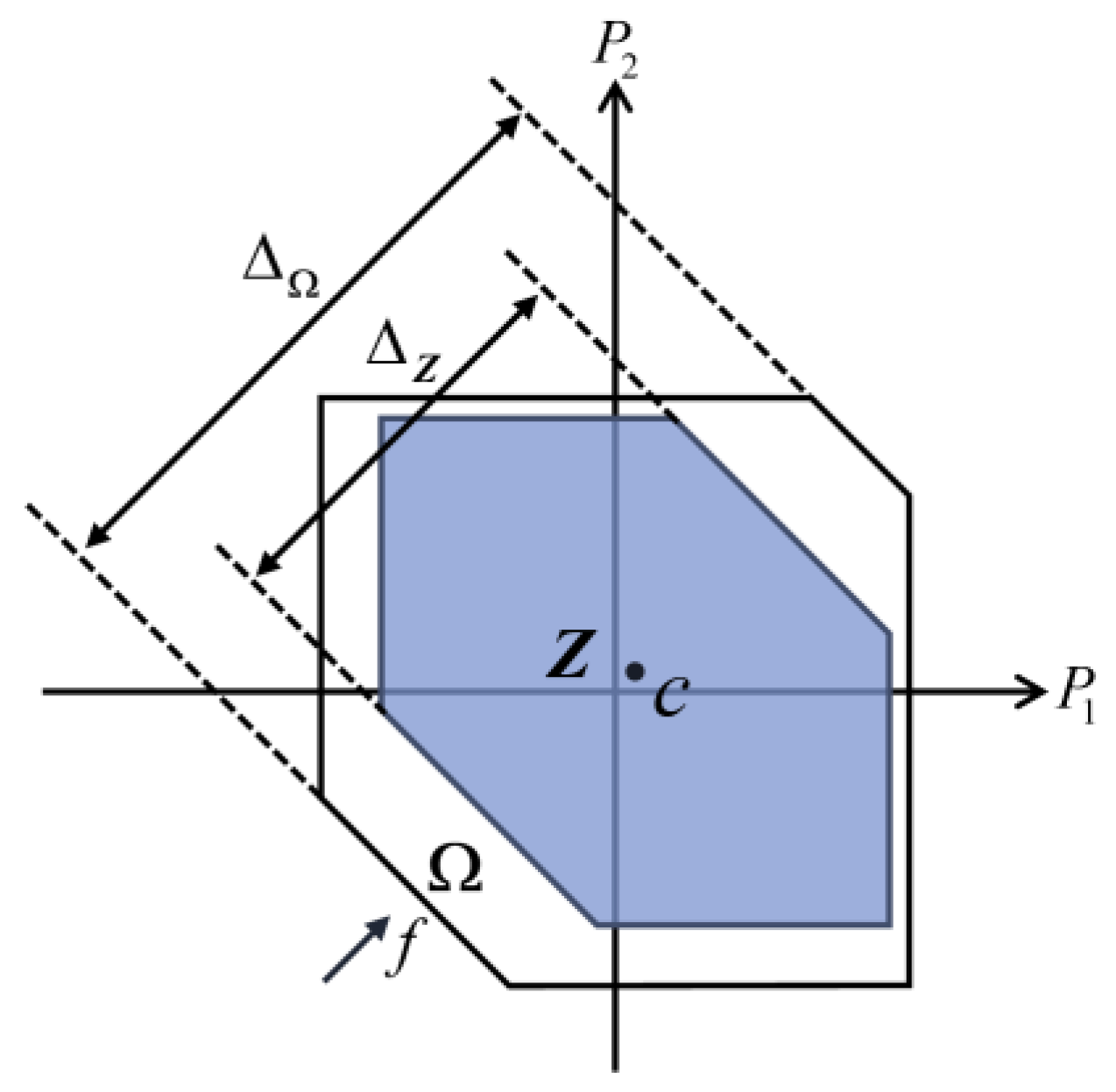
2.2. Characterization of Feasible Region for Distributed Energy Storage Clusters Based on Zonotope

To address the intractability of the Minkowski Sum problem mentioned above, an efficient aggregation method based on Zonotope approximation is adopted in this paper. Specifically, the convex polytope shown in Equation (6) is approximated using the Zonotope form presented in Equation (8), and then the approximated Zonotope is aggregated. Unlike conventional polyhedra represented in half-space form (H-representation) or vertex form (V-representation), Zonotope is a polyhedron with a specific mathematical expression (Z-representation) [12], which is formulated as follows:

$$\mathit{Z}=\{\mathit{x}\in {\mathrm{R}}^N:\mathit{x}=\mathit{c}+\mathit{G}\mathit{\beta },-\overline{\mathit{\beta }}\le \mathit{\beta }\le \overline{\mathit{\beta }}\}$$

(8)

$$\mathit{G}=[{\mathit{g}}^{(1)},{\mathit{g}}^{(1)},\cdots ,{\mathit{g}}^{(M)}]\in {\mathrm{R}}^{N\times M}$$

(9)

$${‖{\mathit{g}}^{(m)}‖}_2=1 m=1,2,\cdots ,M$$

(10)

$$\mathit{\beta }={[{\beta }_1,{\beta }_1,\cdots ,{\beta }_M]}^{\mathrm{T}}$$

(11)

where N is the spatial dimension; c is the coordinates of the centroid of the polyhedron; G is the generator matrix, consisting of M generator vectors ${\mathit{g}}^{(m)}$, representing the extension of the polyhedron from the centroid in all directions; $\mathit{\beta }$ is the extension length of the generator in all directions, limited by the maximum extension length $\overline{\mathit{\beta }}$; ${‖·‖}_2$ denotes the 2-paradigm operation.

In the problem of zonotope approximation for the feasible region of DES, the generator matrix G is considered as a known parameter. The corresponding generator matrices are designed for the power and energy constraints of DES devices, as shown below:

$${\mathit{g}}^{(m)}={[0,\cdots ,0,\underset{m}{\underbrace{ 1 }},0,\cdots ,0]}^{\mathrm{T}} m=1,2,\cdots ,N$$

(12)

$${\mathit{g}}^{(N+m)}={[0,\cdots ,0,\underset{m}{\underbrace{ {\displaystyle \frac{-1}{\sqrt{2}}} }},\underset{m+1}{\underbrace{ {\displaystyle \frac{1}{\sqrt{2}}} }},0,\cdots ,0]}^{\mathrm{T}} m=1,2,\cdots ,N-1$$

(13)

where Equation (12) comprises the first N generators, corresponding to the N power constraints of the DES; Equation (13) includes N-1 generators, corresponding to the N-1 energy constraints of the DES. Consequently, the resulting generator matrix is $\mathit{G}\in {\mathrm{R}}^{N\times (2N-1)}$.

For zonotopes with the same generator matrix G selected, the Minkowski Sum process for these zonotopes is simplified due to their identical extension directions:

$${\mathit{Z}}^{agg}={\mathit{Z}}_1\oplus {\mathit{Z}}_1\cdots \oplus Z_n$$

(14)

$${\mathit{c}}^{agg}={\displaystyle \sum _{r=1}^{N_c}{\mathit{c}}_r}$$

(15)

$${\mathit{\beta }}_m^{agg}={\displaystyle \sum _{r=1}^{N_c}{\beta }_{m,r}}$$

(16)

where ${\mathit{Z}}^{agg}$ is the total zonotope after aggregation; $N_c$ is the number of feasible domains for aggregation, i.e., the number of aggregated resources; ${\mathit{c}}^{agg}$ is the centroid coordinates of the aggregated zonotope; ${\mathit{c}}_r$ is the coordinates of the r-th centroid; ${\mathit{\beta }}_m^{agg}$ is the total extension length in the direction of the m-th generator of the aggregated zonotope; and ${\beta }_{m,r}$ is the extension length of the r-th zonotope in the direction of the m-th generator before aggregation.

It can be observed that the Minkowski Sum process for Zonotopes is a simple linear superposition process, which is attributed to its specific mathematical representation. Thus, the expression of the zonotope is employed to approximate the characterization of the device’s feasible region, transforming from the form of Equation (6) to that of Equation (8). This issue can be modeled as an optimization problem [33], as outlined in the following modeling process:

• Objective functions

A feasibility approximation index $\mathrm{\Lambda }$ is defined to measure the difference between the approximate and original feasible regions of individual DES resources. In a two-dimensional space example, the similarity between the approximate and original feasible regions is illustrated in Figure 1. In the figure, $\mathbf{\Omega }$ represents the original feasible region of an individual DES, and $\mathit{Z}$ represents the approximate feasible region. Several unit normal vectors are selected to represent a specific direction of the feasible region, and the ratio of the widths of $\mathit{Z}$ and $\mathbf{\Omega }$ in each direction is calculated to assess the approximation degree.

$$\mathrm{\Lambda }={\displaystyle \frac{1}{N_f}}{\displaystyle \sum _{k=1}^{N_f}\frac{{\mathsf{\Delta }}_{\mathit{Z},k}}{{\mathsf{\Delta }}_{\mathsf{\Omega },k}}}\in [0,1]$$

(17)

where $N_f$ is the number of unit normal vectors; ${\mathsf{\Delta }}_{\mathbf{\Omega },k}$ and ${\mathsf{\Delta }}_{\mathit{Z},k}$ are the widths of the original feasible domain and the approximate feasible domain in the direction of the k-th unit normal vector, respectively. The DES feasible domain consists of power boundary and energy boundary constraints, and each normal vector can describe the upper and lower bounds of a power or energy boundary constraint, so in the N-dimensional space, 2N-1 normal vectors are selected.

For the calculation of the width of the zonotope in all unit normal vector directions ${\mathsf{\Delta }}_{\mathit{Z}}$ is known from mathematical derivation:

$${\mathsf{\Delta }}_{\mathit{Z}}=2\left|{\mathit{F}}^{\mathrm{T}}\mathit{G}\right|\overline{\mathit{\beta }}$$

(18)

where $\mathit{F}$ is the matrix consisting of the $N_f$ normal vectors.

Substituting Equation (18) into (17) to obtain the objective function is done as follows:

$$\max {\displaystyle \frac{2}{N_f}}{(1/{\mathsf{\Delta }}_{\mathsf{\Omega }})}^{\mathrm{T}}{\left|{\mathit{F}}^{\mathrm{T}}\mathit{G}\right|}^{\mathrm{T}}\overline{\mathit{\beta }}$$

(19)

2.

Calculation of parameters related to the original feasible region approximation index

Let ${\mathsf{\Delta }}_{\mathbf{\Omega }}$ be the maximum distance between two tangent planes of the original feasible domain in each unit normal vector direction, which can be solved by optimization methods. The primal feasible domain $\mathbf{\Omega }$ is represented by a half-space form polyhedron as follows:

$$\mathbf{\Omega }=\left\{\mathit{x}\in {\mathbf{R}}^N:\mathit{A}\mathit{x}\le \mathit{b}\right\}$$

(20)

for a certain unit normal vector $f_k=[a_1,a_2,\cdots ,a_N]$, and its corresponding N-dimensional hyperplane is given by the following:

$$a_1{x}_1+a_2{x}_2+\cdots +a_N{a}_N+b_l=0$$

(21)

where $x_1,x_2,\cdots ,x_N$ is the position in each dimension and $b_l$ is a constant.

This unit normal vector $f_k$ on ${\mathsf{\Delta }}_{\mathbf{\Omega },k}$ can be solved according to the following optimization model:

$$\left\{\begin{array}{ll}\multicolumn{2}{c}{\max {\mathsf{\Delta }}_{O,k}=\left|a_1(x_{1p}-x_{1q})+\cdots +a_N(x_{Np}-x_{Nq})\right|}\\ \begin{array}{cc}\mathrm{s}.\mathrm{t}.& \mathit{A}{\mathit{X}}_P\le \mathit{b}\\ & \mathit{A}{\mathit{X}}_Q\le \mathit{b}\end{array}\end{array}\right.$$

(22)

where ${\mathit{X}}_{\mathit{P}}=[x_{1p},x_{2p},\cdots ,x_{Np}]$ and ${\mathit{X}}_{\mathit{Q}}=[x_{1q},x_{2q},\cdots ,x_{Nq}]$ denote a point outside the hyperplane and a point inside the hyperplane, respectively.

3.

Constraints

The constraint is that the approximated zonotope is inside the feasible domain of the original device. According to the mathematical derivation in Ref. [33], the constraints of this optimization problem are (23), i.e.,

$$\mathit{Z}(\mathit{G}\mathbf{,}\mathit{c}\mathbf{,}\overline{\mathit{\beta }})\in \mathbf{\Omega }(\mathit{A}\mathbf{,}\mathit{b})\iff \mathit{A}\mathit{c}+\left|\mathit{A}\mathit{G}\right|\overline{\mathit{\beta }}\le \mathit{b}$$

(23)

In summary, the zonotope-based device approximate feasible domain optimization model is as follows:

$$\left\{\begin{array}{l}\underset{\left\{\overline{\mathit{\beta }}\right\}}{\max }{\displaystyle \frac{2}{N_f}}{(1/{\mathsf{\Delta }}_{\mathsf{\Omega }})}^{\mathrm{T}}{\left|{\mathit{F}}^{\mathrm{T}}\mathit{G}\right|}^{\mathrm{T}}\overline{\mathit{\beta }}\\ \mathrm{s}.\mathrm{t}. \mathit{A}\mathit{c}+\left|\mathit{A}\mathit{G}\right|\overline{\mathit{\beta }}\le \mathit{b}, \overline{\mathit{\beta }}\ge 0\end{array}\right.$$

(24)

After completing the feasible region approximation, the feasible region of the aggregated cluster can be obtained according to Equations (14)–(16):

$${\mathit{Z}}^{agg}=\{\mathit{x}\in {\mathrm{R}}^N:\mathit{x}={\mathit{c}}^{agg}+\mathit{G}\mathit{\beta },-{\overline{\mathit{\beta }}}^{agg}\le \mathit{\beta }\le {\overline{\mathit{\beta }}}^{agg}\}$$

(25)

3. Multi-Time Scale Hierarchical Coordinated Optimization Strategy for Distribution Networks with Aggregated Distributed Energy Storage

The time scales in the multi-time scale scheduling framework for DNs with aggregated DES, as designed in this study, are introduced as follows:

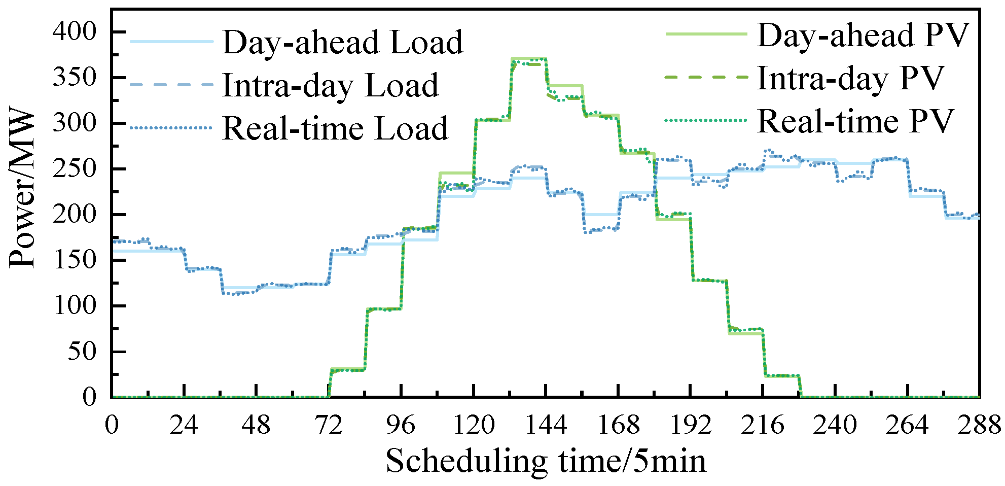
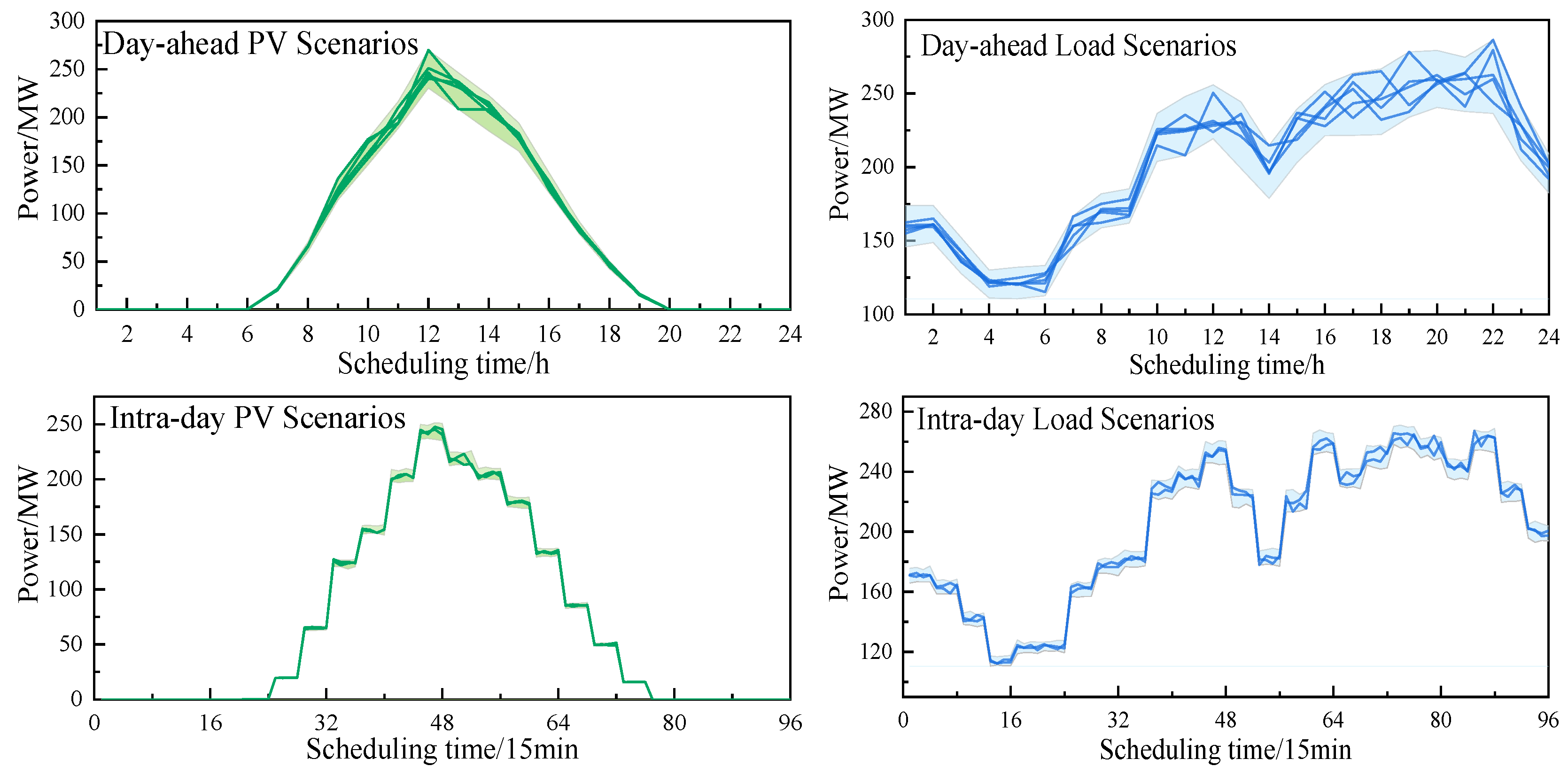
• Day-ahead scheduling: The time scale is set to 1 h, with a scheduling period of 24 h. Considering the wear and tear costs associated with frequent and rapid adjustments of controllable generation units, gas turbines (GTs) are controlled once per hour in the day-ahead scheduling. The day-ahead scheduling determines the on/off states of GTs, power purchase plans from the upstream grid, the participation schedules of DES clusters at each node, and their participation quantities. These determined quantities are then directly fed into the intra-day rolling optimization as fixed variables.
• Intra-day rolling optimization: The time scale is set to 15 min, with an execution cycle of 4 h. During each control cycle, imbalance caused by the output fluctuations of renewable energy units, as well as the load fluctuations of users, is balanced by adjustments from ESS, GTs, and power purchases. In the intra-day scheduling, the on/off states of ESS need to be determined to correct deviations between the day-ahead scheduling plans and actual conditions.
• Real-time coordinated control: The execution cycle is set to 5 min. The objective is to use the intra-day rolling optimization curve as a reference and to implement real-time coordinated control strategies to correct actual operating conditions and minimize deviations.

3.1. Day-Ahead Optimal Scheduling Model

According to existing research, a multi-scenario stochastic optimization method suitable for handling uncertainties is adopted for day-ahead scheduling.

3.1.1. Objective Function

To enhance the accommodation capability of renewable energy, improve power supply reliability under emergency conditions, and better control system carbon emissions, the objective function of the day-ahead scheduling model is formulated to minimize the total operating cost of the system. This is achieved by incorporating the penalty costs associated with PV curtailment and load shedding into the system operating cost, while also accounting for the depreciation cost of ESS. Additionally, a stepped carbon emission cost model is employed. The specific calculation is as follows:

$$\min f_1={\displaystyle \sum _{t=1}^{24}(f_{\mathrm{G},t}+f_{\mathrm{ESS},t}+f_{\mathrm{DG},t}+f_{\mathrm{load},t}+f_{\mathrm{buy},t}+f_{\mathrm{des},\mathrm{t}})}+f_{\mathrm{CO}2}$$

(26)

$$\begin{array}{l}{f}_{\mathrm{G},t}=[{\displaystyle \sum _{s=1}^{N_{\mathrm{S}}}{\displaystyle \sum _{i=1}^{N_{\mathrm{G}}}{p}_s(a_i{P}_{\mathrm{G}i,t,s}^2+b_i{P}_{\mathrm{G}i,t,s}+c_i)}}]+S_i(1-u_{Gi,t-1})u_{Gi,t}\\ f_{\mathrm{ESS},t}={\displaystyle \sum _{s=1}^{N_{\mathrm{S}}}{\displaystyle \sum _{i=1}^{N_{\mathrm{ESS}}}{p}_s[C_{\mathrm{ESS},i}{P}_{\mathrm{ESS},i,t,s}+W_{\mathrm{ESS},i}{P}_{\mathrm{ESS},i,t,s}+{\pi }_{\mathrm{ESS}}{u}_{\mathrm{ESS},i,t,s}]}}\\ f_{\mathrm{DG},t}={\displaystyle \sum _{s=1}^{N_{\mathrm{S}}}{\displaystyle \sum _{i=1}^{N_{\mathrm{DG}}}{p}_s[C_{\mathrm{DG},i}{P}_{\mathrm{DG},i,t,s}+k_{c,\mathrm{DG}}(P_{\mathrm{DG},i,t,s}^{\mathrm{pre}}-P_{\mathrm{DG},i,t,s})]}}\\ f_{\mathrm{load},t}={\displaystyle \sum _{s=1}^{N_{\mathrm{S}}}{p}_s{k}_{c,\mathrm{load}}{P}_{\mathrm{loss},t,s}}\\ f_{\mathrm{buy},t}=c_{\mathrm{buy},t}{P}_{\mathrm{buy},t}\\ f_{\mathrm{des},\mathrm{t}}={\displaystyle \sum _{s=1}^{N_{\mathrm{S}}}{\displaystyle \sum _{n=1}^{N_{des}}{p}_s(k_{c,\mathrm{des}}\left|P_{\mathrm{des},n,t}\right|+c_{\mathrm{des},n}{u}_{\mathrm{des},n})}}\end{array}$$

(27)

where $f_1$ represents the objective function of the day-ahead scheduling optimization model, which denotes the system operating cost; $f_{\mathrm{G},t}$, $f_{\mathrm{erss},t}$, $f_{\mathrm{DG},t}$, $f_{\mathrm{load},t}$, and $f_{\mathrm{des},\mathrm{t}}$ represent the cost functions for GTs, ESS, PV, user load shedding, and the regulation of DES clusters, respectively; $N_S$ denotes the number of scenarios; $p_s$ represents the probability coefficient of the s-th scenario; $N_G$ refers to the number of GTs; and $P_{\mathrm{G}i,t,s}$ represents the power output of the i-th GT at time t under the s-th scenario; $a_i$, $b_i$, and $c_i$ represent the power generation cost coefficients of the i-th GT; $S_i$ is the start-stop cost coefficient of the i-th GT; $u_{Gi,t}$ is the start-stop state of the i-th GT at time t, with 1 being the start and 0 being the stop; $N_{\mathrm{ESS}}$ is the number of ESS; $P_{\mathrm{ESS},i,t,s}$ is the amount of power generated by the ESS i under the s-scenario at time t; $C_{\mathrm{ESS},i}$ and $W_{\mathrm{ESS},i}$ represent the operating cost coefficient and maintenance cost coefficient of the ESS i, respectively; ${\pi }_{\mathrm{ESS}}$ represents the depreciation cost coefficient per unit of time of the ESS; $u_{\mathrm{ESS},i,t,s}$ represents the on/off status of ESS i at time t; $N_{\mathrm{DG}}$ is the number of DG; $P_{\mathrm{DG},i,t,s}$ is the output of the i-th DG in scenario s at time t; $C_{\mathrm{DG},i}$ is the operating cost coefficient of the DG i; $k_{c,\mathrm{DG}}$ is the penalty cost coefficient for wind abandonment; $P_{\mathrm{DG},i,t,s}^{\mathrm{pre}}$ is the predicted output of DG in scenario s at time t; $k_{c,\mathrm{load}}$ is the penalty coefficient for loss of power of the loads; $P_{\mathrm{loss},t,s}$ is the amount of power lost by loads in scenario s at time t; $c_{\mathrm{buy},t}$ is the electricity price at moment t; $f_{\mathrm{buy},t}$ is the amount of electricity purchased from the superior grid at moment t; $N_{\mathrm{des}}$ represents the number of nodes containing DES clusters; $k_{c,\mathrm{des}}$ represents the cost of regulating the DES clusters; $P_{\mathrm{des},n,t}$ represents the power of the DES clusters at node n at moment t; $u_{\mathrm{des},n,t}$ represents the state of the DES clusters at node n participating in the regulation, with 1 representing the participation in the regulation, and 0 representing the non-participation in the regulation; $c_{\mathrm{des},n}$ represents the cost of participating in regulation of the DES clusters at node n.

To quantify the economic and environmental value of the operational regulation of DES, a carbon emission cost model is established by dividing carbon emissions into three segments [34]. The baseline method is adopted to allocate carbon emission allowances, and it is approximately assumed that the system carbon emission allowances are proportional to the output of generation units. The calculation formula for the system carbon emission allowance is as follows:

$$E_L={\displaystyle \sum _{t=1}^T\epsilon P_t}$$

(28)

$$P_t={\displaystyle \sum _{i=1}^{N_{\mathrm{G}}}{P}_{\mathrm{G},i,t}}+P_{\mathrm{DG},t}+P_{\mathrm{buy},t}$$

(29)

where $E_L$ is the total carbon emission allowance of the system; T is the length of an operation cycle; $\epsilon$ is the emission allowance per unit of electricity; $P_t$ is the total power generation of all generating units in the system at the moment t.

PV generation, as a clean and environmentally friendly energy source, does not produce carbon emissions. Therefore, the system’s carbon emissions primarily originate from GTs and power purchased from the upstream grid. The formula for calculating the system’s carbon emissions is expressed as follows:

$$E_{\mathrm{p}}={\displaystyle \sum _{t=1}^T({\displaystyle \sum _{i=1}^{N_{\mathrm{G}}}{\delta }_{Gi}{P}_{\mathrm{G},i,t}}+{\delta }_{Bi}{P}_{\mathrm{buy},t})}$$

(30)

where $E_{\mathrm{p}}$ is the total system carbon emissions in a dispatch cycle; ${\delta }_{Gi}$ is the carbon intensity of GT unit i; ${\delta }_{Bi}$ is the carbon intensity of purchased electricity.

The carbon emission cost is calculated based on the system’s carbon emission allowance and actual carbon emissions as follows:

$$f_{\mathrm{CO}2}=\left\{\begin{array}{l}\mu (E_{\mathrm{p}}-E_{\mathrm{L}}) E_{\mathrm{p}}\le E_{\mathrm{L}}+d\\ \mu d+(1+k)\mu (E_{\mathrm{p}}-E_{\mathrm{L}}-d) E_{\mathrm{L}}+d\le E_{\mathrm{p}}\le E_{\mathrm{L}}+2d\\ (2+k)\mu d+(1+2k)\mu (E_{\mathrm{p}}-E_{\mathrm{L}}-2d) E_{\mathrm{p}}>E_{\mathrm{L}}+2d\end{array}\right.$$

(31)

where $f_{\mathrm{CO}2}$ is the cost of carbon emissions of the system; $\mu$ is the carbon trading price; d is the length of the carbon emissions interval; k is the growth rate of carbon emissions for every 1-step increase in the carbon trading price. It should be noted that when $E_{\mathrm{p}}\le E_{\mathrm{L}}$, $f_{\mathrm{CO}2}$ is negative, which means that the actual carbon emission of the system is smaller than the system’s quota, and the excess carbon emission quota can be traded in the carbon trading market at the initial carbon emission price, so that the system can obtain carbon benefits.

3.1.2. Constraints

• Power Balance Constraint:

$${\displaystyle \sum _{i=1}^{N_{\mathrm{G}}}{P}_{\mathrm{G}i,t,s}}+{\displaystyle \sum _{i=1}^{N_{\mathrm{DG}}}{P}_{\mathrm{DG}i,t,s}}+{\displaystyle \sum _{i=1}^{N_{\mathrm{ESS}}}{P}_{\mathrm{ESS},i,t,s}}+P_{\mathrm{buy},t}=P_{\mathrm{load},t,s}$$

(32)

where $P_{\mathrm{load},t,s}$ is the load at moment t for scenario s.

2.

GT Operation Constraints:

$$P_{\mathrm{G}i}^{\min }\le P_{\mathrm{G}i,t,s}\le P_{\mathrm{G}i}^{\max }$$

(33)

$$\left\{\begin{array}{l}{P}_{\mathrm{G}i,t,s}-P_{\mathrm{G}i,t-1,s}\le u_{Gi,t}{R}_i\\ P_{\mathrm{G}i,t-1,s}-P_{\mathrm{G}i,t,s}\le u_{Gi,t-1}{R}_i\end{array}\right.$$

(34)

where $P_{\mathrm{G}i}^{\min }$ and $P_{\mathrm{G}i}^{\max }$ are the upper and lower output limits of the i-th GT; $R_i$ is the creep rate of the i-th GT.

3.

PV Output Constraints:

$$0\le P_{\mathrm{DG},i,t,s}\le P_{\mathrm{DG},i,t,s}^{\mathrm{pre}}$$

(35)

where $P_{\mathrm{DG},i,t,s}^{\mathrm{pre}}$ is the predicted value of the output of the i-th PV at the moment t under the s scenario.

4.

ESS Constraints:

$$\left\{\begin{array}{l}{P}_{\mathrm{ESS},i}^{\mathrm{dis}}{u}_{\mathrm{ESS},i,t,s}\le P_{\mathrm{ESS},i,t,s}\le P_{\mathrm{ESS},i}^{\mathrm{cha}}{u}_{\mathrm{ESS},i,t,s}\\ S_{\mathrm{SOC},i}^{\min }\le S_{\mathrm{SOC},i,t,s}\le S_{\mathrm{SOC},i}^{\max }\end{array}\right.$$

(36)

where $P_{\mathrm{ESS},i}^{\mathrm{dis}}$ and $P_{\mathrm{ESS},i}^{\mathrm{cha}}$ are the rated charging power and rated discharging power of the ESS i, respectively; $S_{\mathrm{SOC},i,t,s}$ is the charging state of the ESS i at the moment t under the s-scenario; $S_{\mathrm{SOC},i}^{\min }$ and $S_{\mathrm{SOC},i}^{\max }$ are the upper and lower limits of the charging state of the ESS i.

5.

DN Power Flow Constraints:

$${\displaystyle \sum _{p\in {\mathsf{\Omega }}_n^{+}}{P}_{\mathrm{line},t}^p-{\displaystyle \sum _{q\in {\mathsf{\Omega }}_n^{-}}(P_{\mathrm{line},t}^q-{\tilde{I}}_{\mathrm{line},t}^q{R}_{\mathrm{line}}^q)}=P_{\mathrm{out},t}^n}$$

(37)

$${\tilde{U}}_t^j={\tilde{U}}_t^i-2P_{\mathrm{line},t}^L{R}_{\mathrm{line}}^L+{\tilde{I}}_{\mathrm{line},t}^L{(R_{\mathrm{line}}^L)}^2$$

(38)

$${\tilde{I}}_{\mathrm{line},t}^L={(I_{\mathrm{line},t}^L)}^2,0\le {\tilde{I}}_{\mathrm{line},t}^L\le {\tilde{I}}_{\mathrm{line},\max } \forall L(i,j)\in {\mathsf{\Omega }}_{\mathrm{line}}$$

(39)

$${\tilde{U}}_t^n={(U_t^n)}^2, 0\le {\tilde{U}}_t^n\le {\tilde{U}}_{\max } \forall n\in {\mathsf{\Omega }}_{\mathrm{node}}$$

(40)

$${‖\begin{array}{c}2P_{\mathrm{line},t}^L\\ {\tilde{I}}_{\mathrm{line},t}^L-{\tilde{U}}_t^i\end{array}‖}_2\le {\tilde{I}}_{\mathrm{line},t}^L+{\tilde{U}}_t^i, \forall L(i,j)\in {\mathsf{\Omega }}_{\mathrm{line}}$$

(41)

$$\left|P_{\mathrm{line},t}^L\right|\le P_{\mathrm{line},\max }, \forall L(i,j)\in {\mathsf{\Omega }}_{\mathrm{line}}$$

(42)

where ${\mathsf{\Omega }}_n^{+}$ and ${\mathsf{\Omega }}_n^{-}$ represent the sets of branches starting from and ending at node n in the DN; ${\mathsf{\Omega }}_{\mathrm{node}}$ and ${\mathsf{\Omega }}_{\mathrm{line}}$ denote the sets of nodes and branches in the DN; $P_{\mathrm{out},t}^n$ is the output power of node n at time t; $U_t^n$, $I_{\mathrm{line},t}^L$, $P_{\mathrm{line},t}^L$, and $R_{\mathrm{line}}^L$ represent the voltage at node n, the current, power, and the resistance in branch L at time t; ${\tilde{I}}_{\mathrm{line},\max }$, ${\tilde{U}}_{\max }$ and $P_{\mathrm{line},\max }$ are the upper limits of ${\tilde{I}}_{\mathrm{line},t}^L$, ${\tilde{U}}_t^n$ and $P_{\mathrm{line},t}^L$.

6.

DES Cluster Constraints:

$${\mathit{P}}_{\mathrm{des},n}=c_n^{agg}{u}_{\mathrm{des},n}+\mathit{G}{\mathit{\beta }}_n,-{\overline{\mathit{\beta }}}_n^{agg}{u}_{\mathrm{des},n}\le {\mathit{\beta }}_n\le {\overline{\mathit{\beta }}}_n^{agg}{u}_{\mathrm{des},n}$$

(43)

where ${\mathit{P}}_{\mathrm{des},n}$ is the power matrix of the DES cluster at node n; $\mathit{G}$ is the generator matrix; ${\mathit{\beta }}_n$ is the extension length of the generator in each direction; $c_n^{agg}$ and ${\overline{\mathit{\beta }}}_n^{agg}$ represent the center point coordinates of the aggregated zonotope and the maximum extension length of the generators, respectively.

3.2. Intra-Day Rolling Optimization Scheduling Model

Intra-day rolling optimization scheduling is typically performed by feeding the real-time measured system data under the current state into the intra-day rolling optimization model. The optimal control sequence is then solved by incorporating the forecast data of PV generation and load over the next 4 h with a time scale of 15 min.

3.2.1. Objective Function

The objective function of the intra-day rolling optimization is also designed to minimize the system operating cost. Since the day-ahead scheduling model has already determined the on/off status of GTs, power purchase quantities, and the participation schedules and quantities of DES clusters at each node, the objective function in the rolling optimization model subtracts the start-up and shutdown costs of GTs, power purchase costs, and the regulation costs of the DES clusters.

$$\min f_2={\displaystyle \sum _{t=1}^{24}(f_{\mathrm{G},t}+f_{\mathrm{ESS},t}+f_{\mathrm{DG},t}+f_{\mathrm{load},t})}+f_{\mathrm{CO}2}$$

(44)

$$\begin{array}{l}{f}_{\mathrm{G},t}={\displaystyle \sum _{s=1}^{N_{\mathrm{S}}}{\displaystyle \sum _{i=1}^{N_{\mathrm{G}}}{p}_s(a_i{P}_{\mathrm{G}i,t,s}^2+b_i{P}_{\mathrm{G}i,t,s}+c_i)}}\\ f_{\mathrm{ESS},t}=[{\displaystyle \sum _{s=1}^{N_{\mathrm{S}}}{\displaystyle \sum _{i=1}^{N_{\mathrm{ESS}}}{p}_s[C(P_{\mathrm{ESS},i,t,s})+W(P_{\mathrm{ESS},i,t,s})]+{\pi }_{\mathrm{ESS}}{u}_{\mathrm{ESS},i,t}}}\\ f_{\mathrm{DG},t}={\displaystyle \sum _{s=1}^{N_{\mathrm{S}}}{\displaystyle \sum _{i=1}^{N_{\mathrm{DG}}}{p}_s[C(P_{\mathrm{DG},i,t,s})+k_{c,\mathrm{DG}}(P_{\mathrm{DG},i,t,s}^{\mathrm{pre}}-P_{\mathrm{DG},i,t,s})]}}\\ f_{\mathrm{load},t}={\displaystyle \sum _{s=1}^{N_{\mathrm{S}}}{p}_s{k}_{c,\mathrm{load}}{P}_{\mathrm{loss},t,s}}\end{array}$$

(45)

3.2.2. Constraints

The intra-day rolling model also employs a multi-scenario stochastic programming approach to mitigate the adverse impacts of uncertainties. Therefore, its constraints are generally consistent with those in the day-ahead scheduling model. However, compared to the day-ahead model, the intra-day rolling model does not include the GT start-up and shutdown constraints, power purchase constraints, or DES cluster constraints.

3.3. Real-Time Optimization Scheduling Model

Since the time scale of real-time scheduling is 5 min, higher robustness is required for scheduling decisions. The multi-scenario stochastic programming method, which is suitable for day-ahead and intra-day rolling models, becomes inapplicable. In this study, a chance-constrained approach is employed in the mathematical model. By setting specific constraints, the probability of satisfying these constraints is required to be no less than a certain confidence level.

3.3.1. Objective Function

In day-ahead and intra-day scheduling, the power purchase quantities from the upper-level grid, the on/off status of ESS, the participation schedules and quantities of DES clusters, and the on/off schedules of GTs have already been determined. Therefore, the objective function of real-time scheduling only includes the operating and maintenance costs of ESS, the operating costs of GTs, the operating costs of PV systems, the cost of PV curtailment, the cost of load shedding, and the carbon emission cost.

$$\min f_3={\displaystyle \sum _{t=1}^{24}(f_{\mathrm{G},t}+f_{\mathrm{ESS},t}+f_{\mathrm{DG},t}+f_{\mathrm{load},t})}+f_{\mathrm{CO}2}$$

(46)

$$\begin{array}{l}{f}_{\mathrm{G},t}={\displaystyle \sum _{i=1}^{N_{\mathrm{G}}}(a_i{P}_{\mathrm{G}i,t}^2+b_i{P}_{\mathrm{G}i,t}+c_i)}\\ f_{\mathrm{ESS},t}={\displaystyle \sum _{i=1}^{N_{\mathrm{ESS}}}[C(P_{\mathrm{ESS},i,t})+W(P_{\mathrm{ESS},i,t})]}\\ f_{\mathrm{DG},t}={\displaystyle \sum _{i=1}^{N_{\mathrm{DG}}}[C(P_{\mathrm{DG},i,t})+k_{c,\mathrm{DG}}(P_{\mathrm{DG},i,t}^{\mathrm{pre}}-P_{\mathrm{DG},i,t})]}\\ f_{\mathrm{load},t}=k_{c,\mathrm{load}}{P}_{\mathrm{loss},t}\end{array}$$

(47)

3.3.2. Constraints

In the real-time scheduling model, all constraints remain consistent with those in the day-ahead and intra-day models, except that current and voltage limit constraints are replaced with chance constraints [35]. These constraints are not elaborated further here.

$$\mathrm{Pr}\left\{{\tilde{I}}_{\mathrm{line},\min }\le {\tilde{I}}_{\mathrm{line},t}^L\le {\tilde{I}}_{\mathrm{line},\max }\right\}\ge 1-{\xi }_1 , \forall L(i,j)\in {\mathsf{\Omega }}_{\mathrm{line}}$$

(48)

$$\mathrm{Pr}\left\{{\tilde{U}}_{\min }\le {\tilde{U}}_t^n\le {\tilde{U}}_{\max }\right\}\ge 1-{\xi }_1 , \forall n\in {\mathsf{\Omega }}_{\mathrm{node}}$$

(49)

where $\mathrm{Pr}\left\{·\right\}$ denotes the probability that the condition in parentheses holds; ${\xi }_1$ is the node voltage crossing probability and branch current crossing probability, which characterizes the confidence level of the chance constraint equation.

Since the voltage at each node and the current in each branch fluctuate within a certain range while satisfying a confidence level, the chance constraints in Equations (50) and (51), unlike wind and solar power forecasts, do not need to consider factors such as probability distributions or random variables. For the convenience of calculation and modeling, they can be transformed into the deterministic constraints shown in Equations (52) and (53).

$$\left\{\begin{array}{l}{\tilde{I}}_{\mathrm{line},\min }-a_{j,t}[{\tilde{I}}_{\mathrm{line},\min }-{\tilde{I}}_{\mathrm{line},\min }^{\lim }]\le {\tilde{I}}_{\mathrm{line},t}^L\le {\tilde{I}}_{\mathrm{line},\max }+a_{j,t}[{\tilde{I}}_{\mathrm{line},\max }^{\lim }-{\tilde{I}}_{\mathrm{line},\max }]\\ {\displaystyle \sum _{j=1}^{N_{line}}{\displaystyle \sum _{t=1}^T{a}_{j,t}\le T{N}_{line}{\xi }_1}}\end{array}\right.$$

(50)

$$\left\{\begin{array}{l}{\tilde{U}}_{\min }-b_{i,t}[{\tilde{U}}_{\min }-{\tilde{U}}_{\min }^{\lim }]\le {\tilde{U}}_t^n\le {\tilde{U}}_{\max }+b_{i,t}[{\tilde{U}}_{\max }^{\lim }-{\tilde{U}}_{\max }]\\ {\displaystyle \sum _{i=1}^{N_{bus}}{\displaystyle \sum _{t=1}^T{b}_{i,t}\le T{N}_{bus}{\xi }_1}}\end{array}\right.$$

(51)

where $N_{bus}$ and $N_{line}$ are the number of nodes and branches of the DN; ${\tilde{U}}_{\max }^{\lim }$ and ${\tilde{U}}_{\min }^{\lim }$ are the upper and lower limits of the overrun amplitude when the voltage of node i is overrun, taking 1.1pu and 0.9pu; ${\tilde{I}}_{\mathrm{line},\max }^{\lim }$ and ${\tilde{I}}_{\mathrm{line},\min }^{\lim }$ are the upper and lower limits of the overrun amplitude when the current of branch j is overrun; $a_{i,t}$ and $b_{i,t}$ are the Boolean decision variables for the current amplitude of branch j and the voltage amplitude of node i in the time period of t. The value is set to 1 if overrun is found, and to 0 if overrun occurs. If there is an overrun condition, it is 1, and vice versa, it is 0.

4. Power Allocation Method Within Distributed Energy Storage Aggregates Based on the Water-Filling Algorithm

By solving the above optimization scheduling model, the charge and discharge commands of the DES cluster at each time period can be obtained. In this section, the WFA is adopted to allocate these commands. In the power control decomposition of the DES cluster, if the aggregator receives a charging command $D_t^c$, the following problem is solved to determine the charging power $p_{\mathrm{DESc},t}^r$ of each DES:

$$\min -{\displaystyle \sum _{r\in N}\frac{E_r}{{\eta }_{\mathrm{c}}^r}\log (\frac{E_{\mathrm{DES},t-1}^r}{E_r}+\frac{{\eta }_{\mathrm{c}}^r{p}_{\mathrm{DESc},t}^r\mathsf{\Delta }t}{E_r})}$$

(52)

$$\begin{array}{ll}\mathrm{s}.\mathrm{t}. & 0\le p_{\mathrm{DESc},t}^r\le {\widehat{P}}_{\mathrm{DESc},t}^r,\forall r\\ & p_{\mathrm{agg},t}^{\mathrm{c}}={\displaystyle \sum _{r\in N}{p}_{\mathrm{DESc},t}^r}\le D_t^{\mathrm{c}}\end{array}$$

(53)

where $E_r$ is the capacity of the r-th DES; $p_{\mathrm{agg},t}^c$ is the aggregated charging power at time t; ${\widehat{P}}_{\mathrm{DESc},t}^r=\min \left\{P_{\mathrm{DES},\mathrm{c}}^r,(E_r-E_{\mathrm{DES},t-1}^r)/({\eta }_{\mathrm{c}}^r\mathsf{\Delta }t)\right\}$. Objective function (52) endeavors to maintain a consistent storage level across all DES, with the constraints (53) indicates that partial response is allowed but over-response is prohibited. The solution of the problem can be obtained from the following equation:

$$x_r^{*}=\left\{\begin{array}{ll}0& v\in \left(-\infty ,{\alpha }_r\right]\\ v-{\alpha }_r& v\in \left({\alpha }_r,({\alpha }_r+{\overline{x}}_r)\right)\\ {\overline{x}}_r& v\in \left[({\alpha }_r+{\overline{x}}_r),\infty \right)\end{array}\right.$$

(54)

where $x_r^{*}={\eta }_{\mathrm{c}}^r{p}_{\mathrm{DESc},t}^r\mathsf{\Delta }t/E_r$ represents the SOC added by the r-th DES charging at $p_{\mathrm{DESc},t}^r$ for $\mathsf{\Delta }t$ time; $E_r$ is the capacity of the r-th DES; ${\overline{x}}_r={\eta }_{\mathrm{c}}^r{P}_{\mathrm{DES},\mathrm{c}}^r\mathsf{\Delta }t/E_r$ represents the SOC added by the r-th DES charging at rated power $P_{\mathrm{DES},\mathrm{c}}^r$ for $\mathsf{\Delta }t$ time; ${\alpha }_r=E_{\mathrm{DES},t-1}^r/E_r$ represents the SOC of the r-th DES at the end of the t-1 time period. Writing $x_r^{*}$ as $x_r^{*}(v)$, $x_r^{*}(v)$ is a segmented linear function of 1/v.

$${\displaystyle \sum _{r\in N}\frac{x_r^{*}(v)E_r}{{\eta }_{\mathrm{c}}^r\mathsf{\Delta }t}=p_{\mathrm{agg},t}^{\mathrm{c}}}$$

(55)

Equation (55) has a unique root $v^{\ast }$, which can be found by the WFA in Algorithm 1.

If the aggregator receives a discharging command $D_t^{\mathrm{d}}$, the following problem is solved to determine the discharging power $p_{\mathrm{DESd},t}^r$ of each DES:

$$\min -{\displaystyle \sum _{r\in N}{E}_r{\eta }_{\mathrm{d}}^r\log (1-\frac{E_{\mathrm{DES},t-1}^r}{E_r}+\frac{p_{\mathrm{DESd},t}^r\mathsf{\Delta }t}{{\eta }_{\mathrm{d}}^r{E}_r})}$$

(56)

$$\begin{array}{ll}\mathrm{s}.\mathrm{t}.& 0\le p_{\mathrm{DESd},t}^r\le {\widehat{P}}_{\mathrm{DESd},t}^r,\forall r\\ & p_{\mathrm{agg},t}^d={\displaystyle \sum _{r\in N}{p}_{\mathrm{DESd},t}^r}\le D_t^{\mathrm{d}}\end{array}$$

(57)

where ${\widehat{P}}_{\mathrm{DESd},t}^r=\min \left\{P_{\mathrm{DES},\mathrm{d}}^r,(E_r-E_{\mathrm{DES},t-1}^r){\eta }_d^r/\mathsf{\Delta }t\right\}$, $p_{\mathrm{agg},t}^d$ represents the aggregated discharging power at time t. The solution to the problem can be obtained using the following equation:

$$x_r^{*}=\left\{\begin{array}{ll}0& v\in \left[{\alpha }_r,\infty \right)\\ {\alpha }_r-v& \mathrm{otherwise}\\ {\overline{x}}_r& v\in \left(-\infty ,({\alpha }_r-{\overline{x}}_r)\right]\end{array}\right.$$

(58)

where $x_r^{*}=p_{\mathrm{DESd},t}^r\mathsf{\Delta }t/{\eta }_d^r{E}_r$ denotes the SOC reduced by the time the r-th DES discharges$\mathsf{\Delta }t$ at $p_{\mathrm{DESd},t}^r$; ${\overline{x}}_r=P_{\mathrm{DES},\mathrm{d}}^r\mathsf{\Delta }t/{\eta }_{\mathrm{d}}^r{E}_r$ denotes the SOC reduced by the time the r-th DES discharges $\mathsf{\Delta }t$ at the rated power $P_{\mathrm{DES},\mathrm{d}}^r$; writing $x_r^{*}$ as $x_r^{*}(v)$, $x_r^{*}(v)$ is a segmented linear function of 1/v.

$${\displaystyle \sum _{r\in N}\frac{x_r^{*}(v){\eta }_{\mathrm{d}}^r{E}_r}{\mathsf{\Delta }t}=p_{\mathrm{agg},t}^{\mathrm{d}}}$$

(59)

Similarly, then the decomposition of the discharge power can be solved by the WFA.

Algorithm 1. Water-Filling Algorithm WFA

1.      $\mathrm{Calculate} ({\alpha }_r+{\overline{x}}_r) \mathrm{and} {\alpha }_r$$(\mathrm{when} \mathrm{charging}) \mathrm{or} ({\alpha }_r-{\overline{x}}_r)$$\mathrm{and} {\alpha }_r (\mathrm{when} \mathrm{discharging}) \mathrm{for} \mathrm{all} \mathrm{ESS} \mathrm{in} \mathrm{this} \mathrm{cluster}, \mathrm{merge} \mathrm{the} \mathrm{two} \mathrm{points} \mathrm{with} \mathrm{the} \mathrm{same} \mathrm{value}, \mathrm{and} \mathrm{count} \mathrm{the} \mathrm{total} \mathrm{number} \mathrm{of} \mathrm{breakpoints} \mathrm{as} L. \mathrm{The} \mathrm{sorted} \mathrm{sequence} \mathrm{is} \left\{v_1,v_1,\dots ,v_L\right\}$, which divides the range of v into L + 1 intervals.

2.      $\mathrm{For} \mathrm{each} \mathrm{interval} [{\nu }_j, {\nu }_{j+1}]$

3.            $\mathrm{Based} \mathrm{on} \mathrm{Equations} \left(54\right)/\left(58\right) \mathrm{Calculation} x_r^{*}(v)$

4.            $\mathrm{According} \mathrm{to} \mathrm{Equations} \left(55\right)/\left(59\right) \mathrm{find} \mathrm{the} v^{\ast }$

5.            $\mathrm{if} v^{\ast }\in [{\nu }_j, {\nu }_{j+1}]$

6.                  $\mathrm{Record} v^{\ast }$$\mathrm{and} x_r^{*}(v)$

7.            else

8.                  Update j = j + 1 and return to step 3

9.            end if

10.      end for

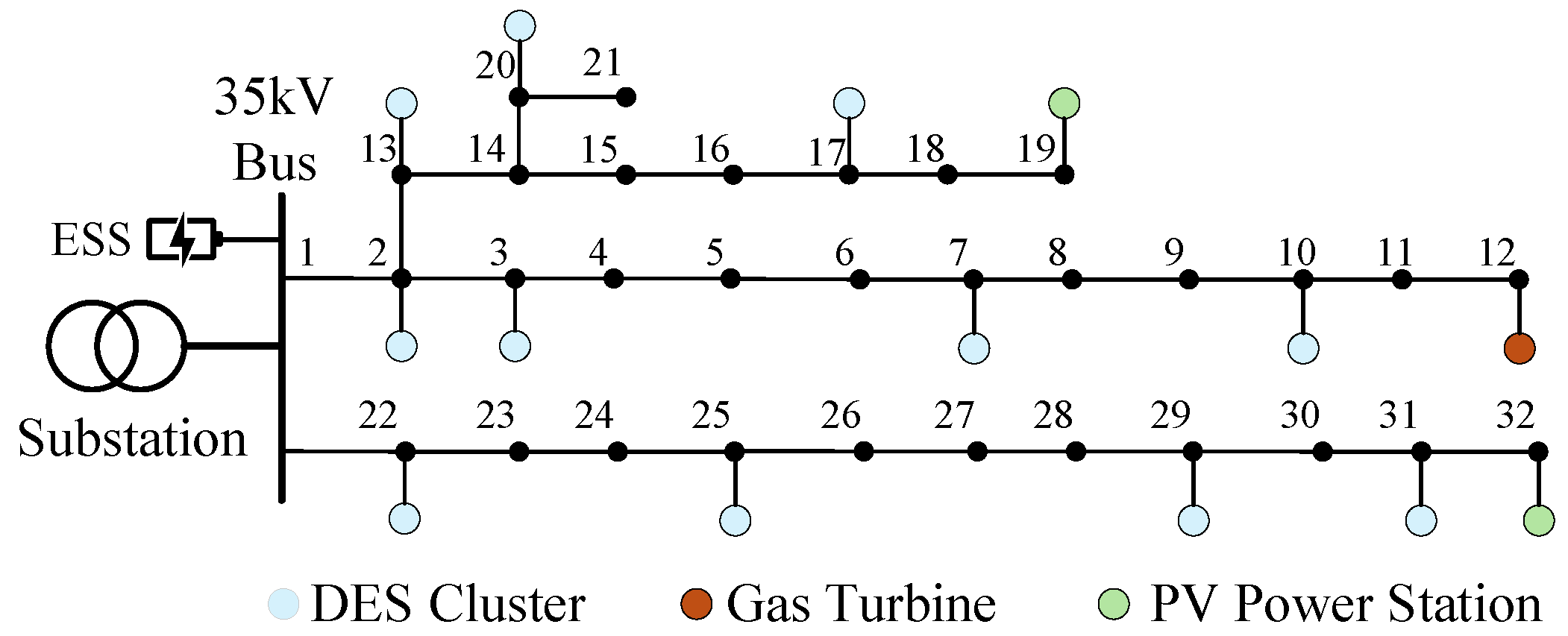
5. Case Studies

In this study, the DN of a demonstration county in China, as shown in Figure 2, is analyzed for verifying the effectiveness of the method proposed in this paper. The DN includes one gas turbine unit located at bus node 12, with the unit parameters provided in

Table 1. Gas turbine parameters.

Pmax/MW	Pmin/MW	a/($/(MW))2	b/($/MW)	C/$	Climbing Rate/(MW/h)	Minimum Switching Time/h
100	10	0.375	400	375	35	2

. The DES clusters are located at bus nodes 2, 3, 7, 10, 13, 17, 20, 22, 25, 29, and 31. Distributed PV systems are installed at all nodes, with PV power stations specifically located at node 19 and node 32. An ESS on the grid side is located at bus node 1. The day-ahead, intra-day, and real-time forecast curves for PV and load are shown in Figure 3. Monte Carlo sampling is employed to generate 200 initial PV output and load scenarios for both day-ahead and intra-day stages. The forecast errors for load are set at 3% and 1% for the day-ahead and intra-day stages, respectively, while the forecast errors for PV are set at 5% and 3%, respectively. Next, the initial scenario sets are reduced using a fast non-dominated sorting technique based on probability distance, resulting in 5 day-ahead scenarios and 2 intra-day scenarios. The typical scenario generation results for PV and load are shown in Figure 4. From Figure 4, it can be seen that PV output power is peaked between 11:00 AM and 1:00 PM, reflecting the typical pattern driven by maximum sunlight exposure. In contrast, the load is varied throughout the day and is peaked between 9:00 PM and 10:00 PM, due to increased residential energy consumption for lighting and appliances. Between 3:00 AM and 6:00 AM, the load is reduced to a low point as most activities are paused. At midday, PV output power is exceeded over the load, which could result in power backflow and challenges in accommodating the PV output efficiently. The model was constructed as a mixed-integer second-order cone optimization problem using the YALMIP toolbox on the MATLAB platform, and it was solved using the GUROBI solver. A flexible and intuitive interface for modeling optimization problems was provided by YALMIP, while GUROBI’s efficiency and reliability aided in successfully addressing the large-scale optimization task.

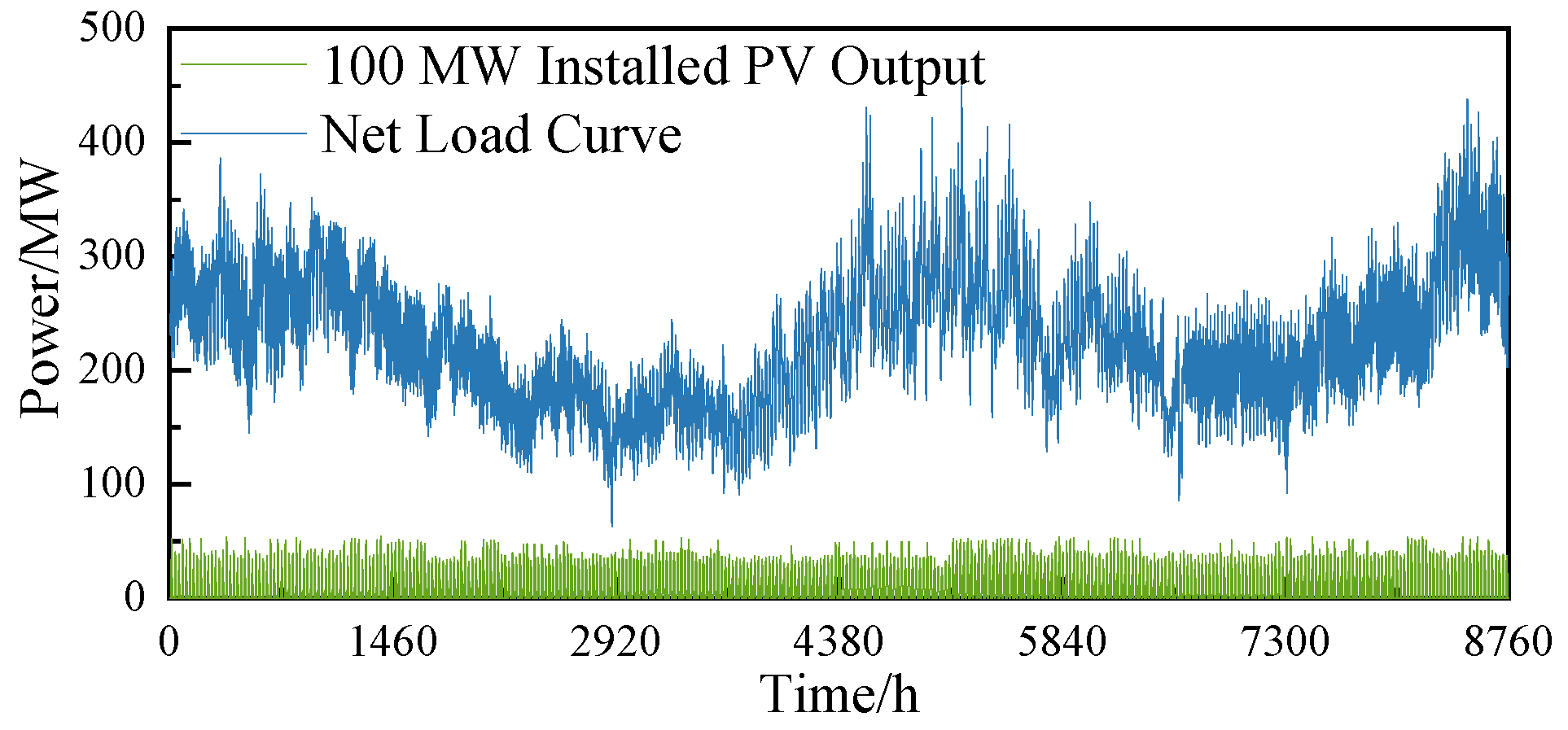
5.1. Regulation Requirements of Distributed Energy Storage

The regulation requirements of DES for rapid ramping, intra-day load balancing, and peak supply assurance have been analyzed in the context of modern power systems with widespread renewable energy integration.

In Figure 5, the annual PV curve with an installed capacity of 100 MW for the demonstration county is presented. During this period, the intra-day hourly-level flexible ramping demand of the power system can reach up to 21.84 MW. In Figure 1, the 2023 net load curve for the demonstration county is shown, with a maximum daily load peak-to-valley difference of approximately 183.8 MW, accounting for 62.35% of the daily maximum load (referred to as the daily maximum peak-to-valley difference rate). For the year 2023, the maximum load of the county is projected to be 449.8 MW. Under the constraint of a 13% system reserve margin, the installed capacity of wind power in the demonstration county is assumed to be 750 MW, and the installed capacity of PV is assumed to be 1142.6 MW. Using assumptions of an effective capacity factor of 35% for wind power and 20% for PV, the power supply assurance demand during peak periods in 2023 is estimated to be approximately 17.254 MW.

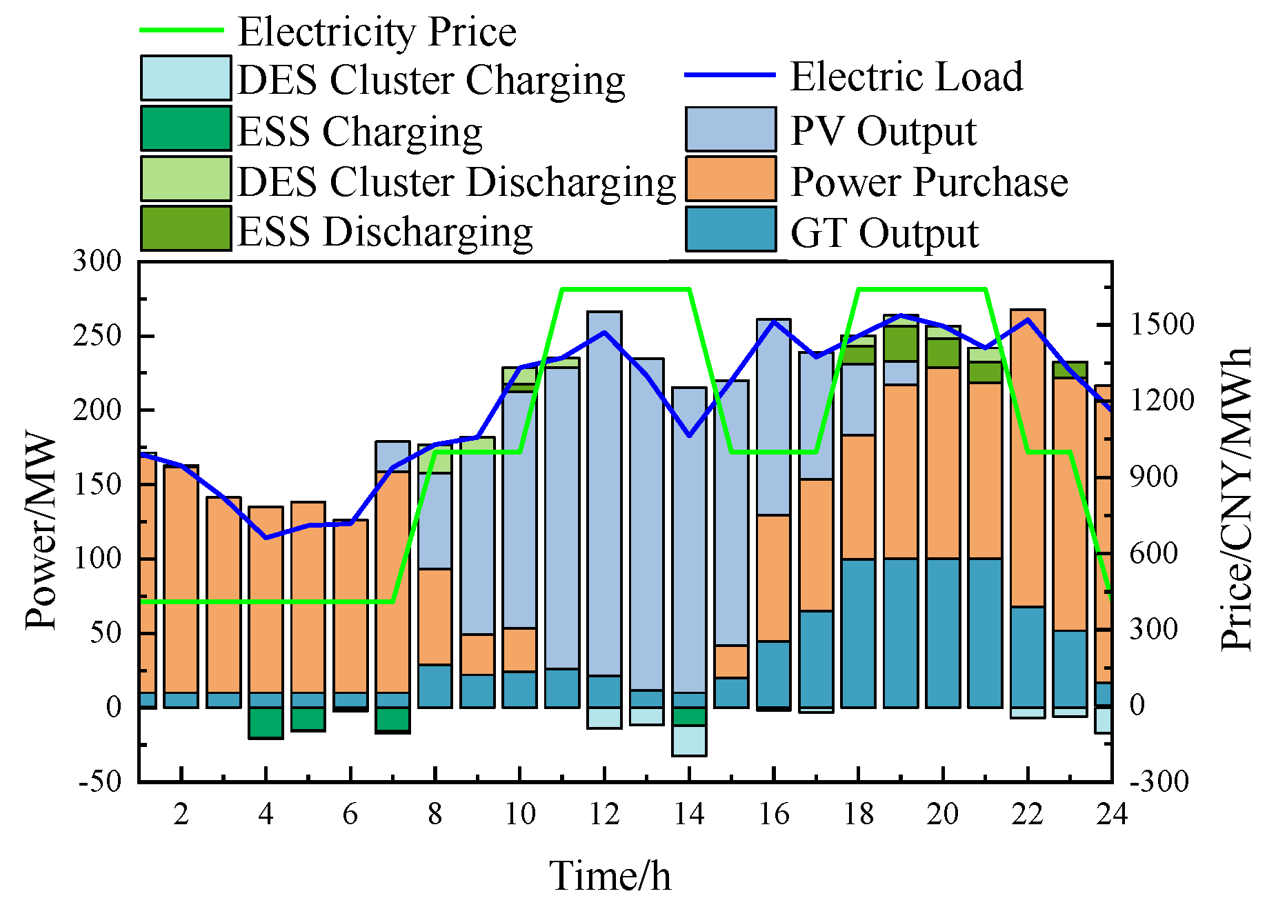
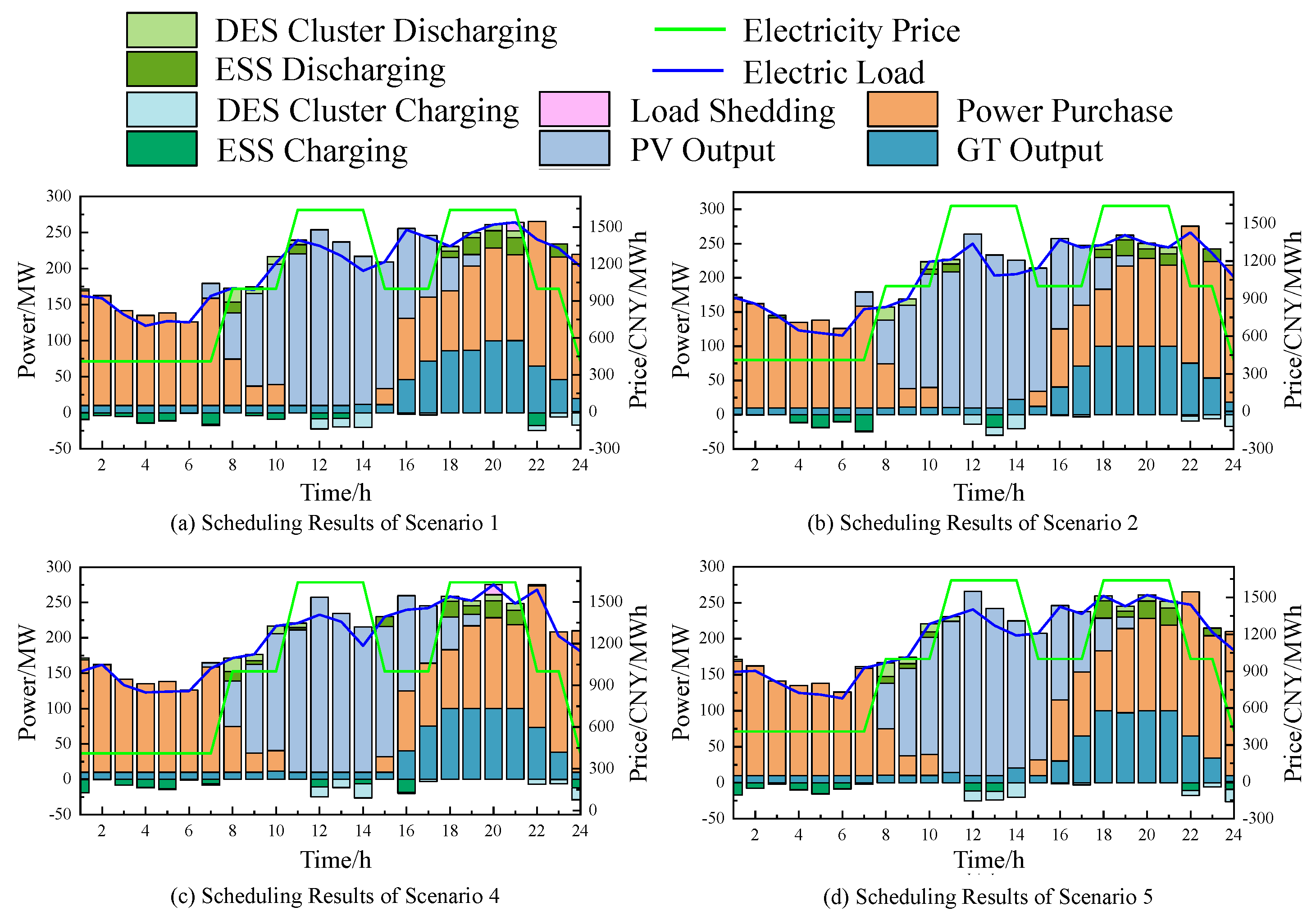
5.2. Analysis of Day-Ahead Scheduling Results

Table 2. Probabilities of Day-Ahead PV Output and Load for Each Scenario.

Scenarios	Probabilities
1	0.01
2	0.22
3	0.455
4	0.125
5	0.19

presents the probabilities of the five day-ahead scenarios. Based on these scenarios, a stochastic optimization method is used to solve the day-ahead scheduling model, considering the uncertainties of PV and load. The scheduling results are shown in Figure 6 and Figure 7. Figure 6 illustrates the results for the scenario with the highest probability, Scenario 3. During the early morning period (0:00–6:00), when the load is low and electricity prices are low, PV output is 0. The system primarily relies on power purchases from the upper-level grid to meet the load demand, and surplus power is used to charge the ESS. As time approaches the morning peak, gas turbine output gradually increases, and PV begins to contribute to the power supply. In the morning period (6:00–10:00), PV output gradually increases, reducing reliance on other power sources. During this period, external power purchases are minimized, and as the load rises, the DES clusters and ESS discharge to reduce system operating costs. During the midday period (10:00–14:00), PV maintains high output, and no external power purchases are needed. Surplus PV power is used to charge the ESS and DES clusters, improving the accommodation rate of renewable energy. In the evening peak period (17:00–21:00), electricity prices rise as demand increases, PV output decreases, and GT output ramps up. This is supplemented by discharges from the ESS, DES clusters, and external power purchases to meet the demand. Flexible scheduling ensures both economic efficiency and a reliable power supply. Figure 7 shows the scheduling results for the other four possible scenarios. Since day-ahead scheduling fixes the power purchase quantities, on/off states of GTs, and outputs of DES clusters to be used in the intra-day and real-time models, these parameters remain identical across all scenarios. In Scenarios 1 (20:00–21:00) and 4 (19:00–20:00), high load periods occur when GT output reaches its maximum limit, resulting in a small amount of load shedding. To meet the load demand, adjustments to power purchase quantities are needed in the intra-day stage. The scheduling results for Scenarios 2 and 5 are similar to Scenario 3 and are not further detailed here.

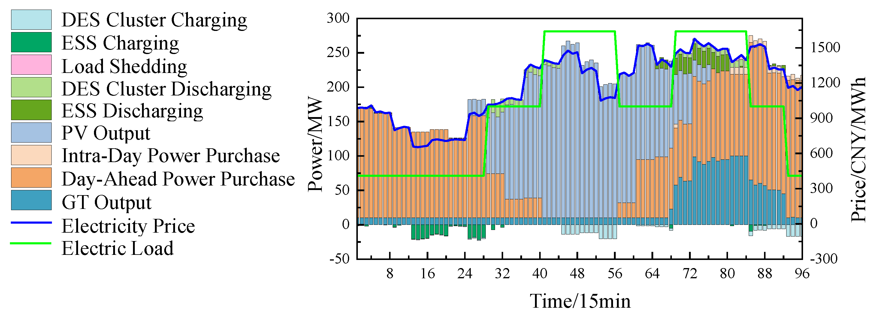
5.3. Analysis of Intra-Day Scheduling Results

Based on the two sets of scenarios generated for the intra-day stage, a stochastic optimization method is utilized to solve the intra-day optimization scheduling model, which considers the uncertainties of PV and load. As shown in

Table 3. Intra-day PV output and load probability of each scenario.

Scenarios	Probabilities
1	0.565
2	0.435

, the probability of Scenario 1 is 0.565, and the probability of Scenario 2 is 0.435. In this process, the power purchase quantities, GT on/off states, and the outputs of DES clusters determined in the day-ahead optimization are adopted. The scheduling results for each scenario are shown in Figure 8 and Figure 9, and they are generally consistent with the results of Scenario 3 in the day-ahead stage. However, during the period from 20:00 to 24:00, due to the uncertainty in load, the power purchase quantities determined in the day-ahead stage are insufficient to meet the demand, requiring adjustments to the power purchase quantities in the intra-day stage to satisfy the increased load.

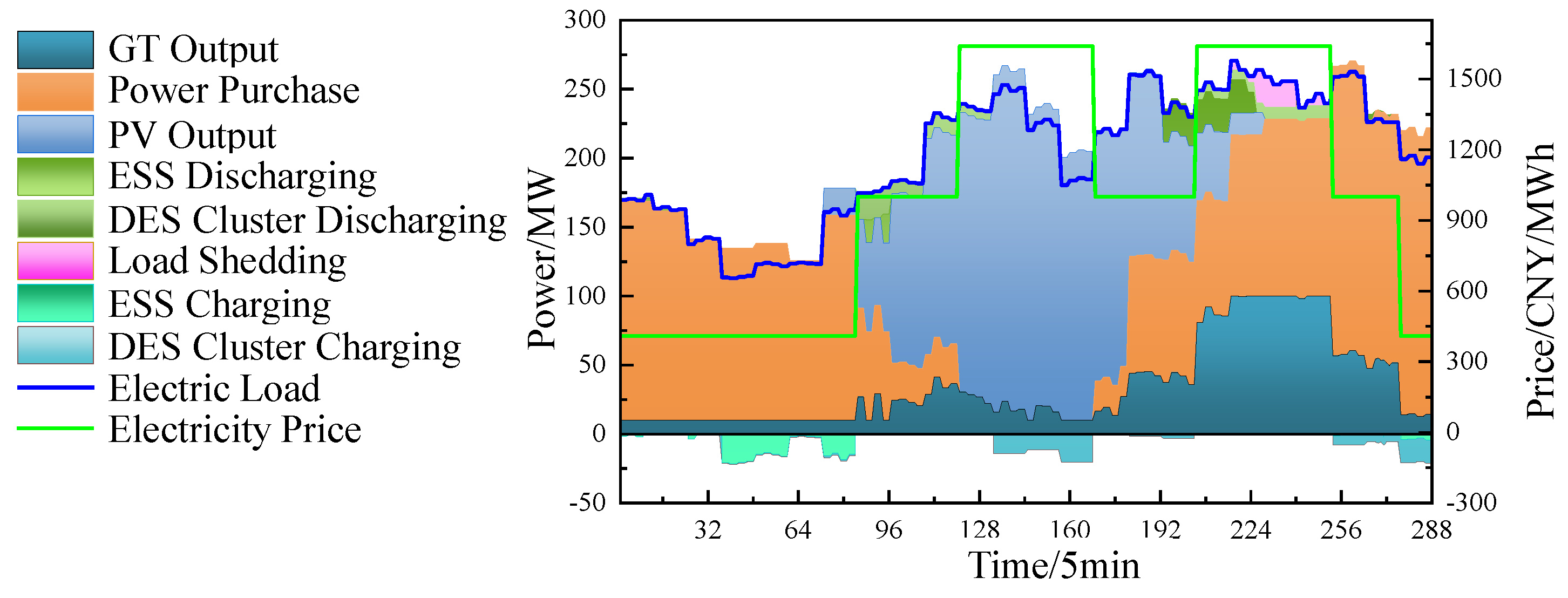
5.4. Real-Time Scheduling Results

The real-time scheduling results shown in Figure 10 indicate that GT and power purchases provide a stable foundation for electricity supply, while PV reaches its peak during the midday period. ESS are charged during periods of low electricity prices at night and high PV output at midday. During peak load periods, ESS actively discharge, alleviating the pressure on power supply and reducing the amount of load shedding.

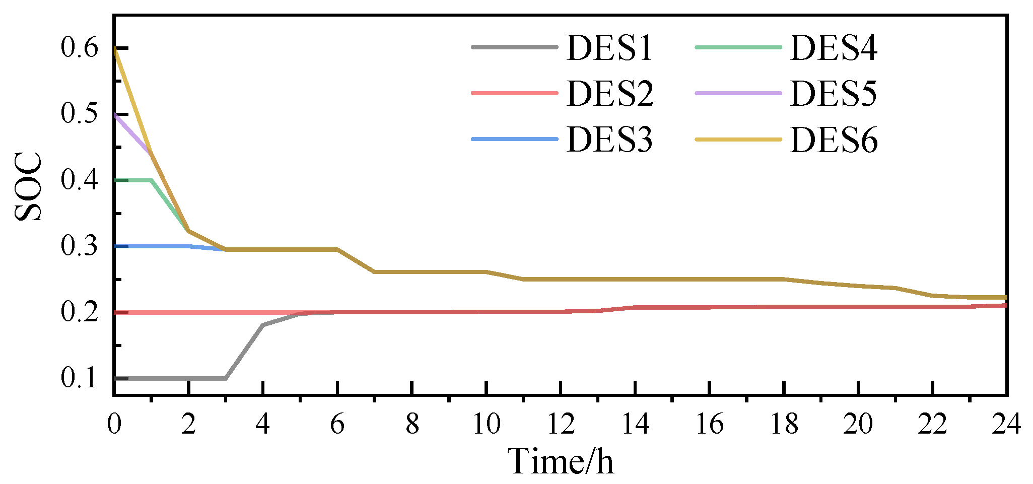
5.5. Power Decomposition Results of Distributed Energy Storage Clusters

Due to the large number of DES devices, the power decomposition results of six representative devices are selected for demonstration in this paper. Figure 11 illustrates the power decomposition results of these six DES units and shows the SOC trends during the scheduling period. It can be observed that, from 00:00 to 03:00, the DES cluster operates under discharge commands. DES4–DES6, which have higher initial SOC levels, discharge during this period, and DES units with higher initial SOC are allocated more discharge power. DES1–DES3, with lower initial SOC levels, do not discharge during this time. From 03:00 to 06:00, the cluster operates under charge commands. DES1, with the lowest initial SOC, charges during this period, while DES2–DES5, with relatively higher SOC levels at the time, do not charge. By the end of the third time interval, the SOC levels of DES3–DES6, which started with higher initial SOC, have converged to similar values. Similarly, by the end of the fifth time interval, the SOC levels of DES1–DES2, which started with lower initial SOC, also converge. Over time, the SOC levels of all DES units gradually become consistent. This power decomposition method effectively coordinates all DES units within the cluster, ensuring that their SOC levels closely align and thereby maximizing the retention of overall power flexibility.

5.6. Analysis of the Regulation Efficiency of Distributed Energy Storage

5.6.1. Supply Assurance Effect

To comprehensively evaluate the impact of DES regulation on the supply assurance capability of the DN based on its ability to handle sudden load changes and fault recovery, it is assumed that a sudden load increase occurs during the 19:00 to 20:00 period, resulting in a load shedding of 20.72 MW, as shown in

Table 4. Supply Assurance Effect Before and After DES Integration.

Scenarios	Voltage Overrun	Power Overrun	Overload
Before DES Integration	2.47%	0.65%	6.46%
After DES Integration	0%	0%	0%

, with a load shedding severity of 6.46%. Meanwhile, the power overload severity reaches 0.65%, and the most severe voltage limit violation occurs between 22:00 and 23:00, reaching 2.47%. After the introduction of DES, these issues are eliminated, significantly improving the power supply capability and security of the DN. Through intelligent dispatch and rapid response strategies, the energy storage system effectively addresses load fluctuations, enhancing the dynamic support capability of the system and reducing voltage and power limit violations. This demonstrates that DES plays a critical role in enhancing the flexibility and stability of grid operation under high-load conditions, providing essential support for the integration of renewable energy.

5.6.2. Accommodation Effect

The effect of DES regulation on promoting renewable energy accommodation is analyzed based on the accommodation performance of renewable energy. As shown in

Table 5. Renewable Energy Accommodation Effect in Each Scenario Before and After DES Integration.

Scenarios	Accommodation Rate Before DES Integration	Accommodation Rate After DES Integration
1	95.90%	100%
2	96.67%	100%
3	97.36%	100%
4	96.20%	99.14%
5	96.58%	98.95%

, the introduction of the energy storage system significantly improves the accommodation of renewable energy. Before the participation of energy storage, the accommodation rates across the scenarios were 95.90%, 96.67%, 97.36%, 96.20%, and 96.58%, indicating that a portion of renewable energy was not fully utilized. However, after the participation of energy storage, the accommodation rates were significantly improved to 100%, 100%, 100%, 99.14%, and 98.95%. This demonstrates that energy storage substantially enhances the grid’s regulation capability by absorbing excess power and balancing supply and demand. It not only effectively reduces the waste of renewable energy but also increases the efficiency of energy utilization, laying a solid foundation for the further development of renewable energy.

5.6.3. Cost and Environmental Value

In this study, the system operating costs before and after DES participation were calculated, considering the cost of energy storage lifecycle degradation and PV curtailment. A system carbon emission model was established to calculate carbon emissions in the two scenarios. By comparing the operating costs and carbon emissions under these scenarios, the cost and environmental value of DES regulation were quantified. It was assumed that the carbon emission intensities of GT and power purchases in the DN were 0.45 tons/MWh and 0.55 tons/MWh, respectively, while the system’s carbon emission allowance was set at 0.5 tons/MWh. The cost and environmental values before and after DES integration are shown in

Table 6. Economic and Environmental Effects Before and After DES Integration.

Scenarios	Carbon Emission Allowance	Carbon Emissions	Carbon Emission Cost
Before DES Integration	2407.9 T	1633.2 T	−38,736 CNY
After DES Integration	2399.4 T	1607.4 T	−39,605 CNY

. As observed in the table, after the integration of DES, the carbon emission allowance decreased from 2407.9 tons to 2399.4 tons, a reduction of 8.5 tons, while the actual carbon emissions decreased from 1633.2 tons to 1607.4 tons, a reduction of 25.8 tons. This indicates that the DES plays a significant role in reducing carbon emissions. At the same time, carbon emission costs decreased from −38,736 CNY to −39,605 CNY, a reduction of 869 CNY. This adjustment not only reflects cost benefits but also significantly enhances the environmental performance of the system, further supporting the strategic goal of low-carbon operation.

6. Conclusions

To enhance the renewable energy accommodation rate and operational reliability of the DN while reducing operational costs, a multi-time scale hierarchical coordinated optimization strategy for DNs considering the aggregation of DES resources is proposed in this paper. A DES aggregation method based on the inner approximation of the Minkowski Sum is proposed. A power allocation method for DES clusters based on the WFA is proposed. Based on the case study analysis, the following conclusions are drawn:

• Considering the participation of DES resource clusters in the optimal operation of DNs can reduce operational costs, improve the operational reliability of the DN, and enhance the renewable energy accommodation rate.
• The proposed multi-time scale optimization operation method effectively utilizes the fast regulation capabilities of ESS and DES resources, thereby improving the accuracy of the system’s response to forecast data.
• The application of the WFA for decomposing control commands of the DES clusters effectively balances the loads of individual DES units, optimizes resource allocation, and provides a feasible solution for large-scale distributed DES deployment.

In future work, further improvements in the approximation accuracy of the aggregation method will be required, and research on the optimal aggregation scope of DES will be conducted.

References

- Cui, Y.; Zhou, H.; Zhong, W.; Li, H.; Zhao, Y. Low-Carbon Scheduling of Power System with Wind Power Considering Uncertainty of Both Source and Load Sides. Electr. Power Autom. Equip. 2020, 40, 85–93. [Google Scholar]
- Li, J.; Sun, H.; Xu, C.; Jing, X.; Jia, G. Research on Distributed Energy Storage Resource Management and Strategy Participating in Demand Response of New Power Systems. Distrib. Util. 2022, 39, 29–35. [Google Scholar]
- Duan, X.; Wang, Y.; Wei, Y.; Li, Y.; Cui, X. DPV and HESS Joint Optimal Configuration in Distribution Network Considering Renewable Energy Consumption. Mod. Electr. Power, 2024; ahead of print. [Google Scholar] [CrossRef]
- Wang, C.; Shi, Z.; Liang, Z.; Li, Q.; Hong, B.; Huang, B.; Jiang, L. Key Technologies and Prospects of Demand-Side Resource Utilization for Power Systems Dominated by Renewable Energy. Autom. Electr. Power Syst. 2021, 45, 37–48. [Google Scholar]
- Sun, L.; Li, H.; Jia, Q.; Fu, L.; Zhang, G. Planning Method for Resource Aggregation of Virtual Power Plant Based on Dynamic Reconstruction. Autom. Electr. Power Syst. 2024, 48, 115–128. [Google Scholar]
- Zhuang, Y.; Li, Z.; Tan, Q.; Li, Y.; Wan, M. Multi-Time-Scale Resource Allocation Based on Long-Term Contracts and Real-Time Rental Business Models for Shared Energy Storage Systems. J. Mod. Power Syst. Clean Energy 2024, 12, 454–465. [Google Scholar] [CrossRef]
- Kwon, K.; Lee, H.-B.; Kim, N.; Park, S.; Joshua, S.R. Integrated Battery and Hydrogen Energy Storage for Enhanced Grid Power Savings and Green Hydrogen Utilization. Appl. Sci. 2024, 14, 7631. [Google Scholar] [CrossRef]
- Yin, Q. Scale Distributed Energy Storage Aggregation Modeling and Cooperative Optimized Regulation Strategy. Ph.D. Thesis, North China Electric Power University, Beijing, China, 2019. [Google Scholar]
- He, S.; Zhang, J.; Gu, Z.; Shi, X.; Jiang, H. Overview of Virtual Power Plant Modeling and Optimization Control for Distributed Resource Aggregation and Control. Shandong Electr. Power. 2024, 51, 11–24. [Google Scholar]
- Liu, Q.; Yang, S.; Liu, X. Analysis and Prospect of Distributed Energy Storage Business Modes. Power Demand Side Manag. 2023, 25, 67–73. [Google Scholar]
- Wang, S.; Wu, W. Aggregation Reference Model and Quantitative Metric System of Flexible Energy Resources. Autom. Electr. Power Syst. 2024, 48, 1–9. [Google Scholar]
- Zhang, H.; Chang, L.; Cao, L.; Lu, J. Research on Demand Side Resource Feasible Region Aggregation Based on Improved Zonotope. Power Demand Side Manag. 2024, 26, 1–7. [Google Scholar]
- Zhang, L.; Fan, Y.; Wang, Y.; Zhou, B.; Dou, Q. Flexible Aggregation and Coordinated Scheduling Strategy for Renewable Powered 5G Communication Base Station Clusters. Power Syst. Prot. Control. 2024, 52, 101–110. [Google Scholar]
- Barot, S.; Taylor, J.A. A Concise, Approximate Representation of a Collection of Loads Described by Polytopes. Int. J. Electr. Power Energy Syst. 2017, 84, 55–63. [Google Scholar] [CrossRef]
- Zhao, W.; Huang, H.; Zhu, J.; Zhou, B.; Chen, J.; Luo, Y. Flexible Resource Cluster Response Based on Inner Approximate and Constraint Space Integration. Power Syst. Technol. 2023, 47, 2621–2632. [Google Scholar]
- Wen, Y.; Hu, Z.; You, S.; Duan, X. Aggregate Feasible Region of DERs: Exact Formulation and Approximate Models. IEEE Trans. Smart Grid 2022, 13, 4405–4423. [Google Scholar] [CrossRef]
- Chen, X.; Li, N. Leveraging Two-Stage Adaptive Robust Optimization for Power Flexibility Aggregation. IEEE Trans. Smart Grid 2021, 12, 3954–3965. [Google Scholar] [CrossRef]
- Lv, Y.; Li, K.; Zhao, H.; Lei, H. A Multi-Stage Constraint-Handling Multi-Objective Optimization Method for Resilient Microgrid Energy Management. Appl. Sci. 2024, 14, 3253. [Google Scholar] [CrossRef]
- Jin, L.; Fang, X.; Cai, Z.; Chen, D.; Li, Y. Multiple Time-Scales Source-Storage-Load Coordination Scheduling Strategy of Grid Connected to Energy Storage Power Station Considering Characteristic Distribution. Power Syst. Technol. 2020, 44, 3641–3650. [Google Scholar]
- Chen, Y.; Qi, D.; Dong, H.; Li, C.; Li, Z.; Zhang, J. A FDI Attack-Resilient Distributed Secondary Control Strategy for Islanded Microgrids. IEEE Trans. Smart Grid 2021, 12, 1929–1938. [Google Scholar] [CrossRef]
- Dong, W.; Zhang, F.; Li, M.; Fang, X.; Yang, Q. Imitation Learning Based Real-Time Decision-Making of Microgrid Economic Dispatch Under Multiple Uncertainties. J. Mod. Power Syst. Clean Energy 2024, 12, 1183–1193. [Google Scholar]
- Cui, Y.; Zhou, H.; Zhong, W.; Hui, X.; Zhao, Y. Two-Stage Day-Ahead and Intra-Day Rolling Optimization Scheduling Considering Joint Peak Regulation of Generalized Energy Storage and Thermal Power. Power Syst. Technol. 2021, 45, 10–20. [Google Scholar]
- Zhou, H. Optimal Dispatch of Wind Power System Considering Source-Load-Storage Joint Peak Shaving. Ph.D. Thesis, Northeast Electric Power University, Beijing, China, 2021. [Google Scholar]
- Pan, P.; Wang, Z.; Chen, G.; Shi, H.; Zha, X. Multi-Time Scale Optimal Dispatch of Distribution Network with Pumped Storage Station Based on Model Predictive Control. Appl. Sci. 2024, 14, 11122. [Google Scholar] [CrossRef]
- Huang, X.; Qi, D.; Chen, Y.; Yan, Y.; Yang, S.; Wang, Y.; Wang, X. Distributed Self-Triggered Privacy-Preserving Secondary Control of VSG-Based AC Microgrids. IEEE Trans. Smart Grid, 2024; ahead of print. [Google Scholar] [CrossRef]
- Chen, Z.; Li, Z.; Lin, D.; Xie, C.; Wang, Z. Multi-Time-Scale Optimal Scheduling of Integrated Energy System with Electric-Thermal-Hydrogen Hybrid Energy Storage under Wind and Solar Uncertainties. J. Mod. Power Syst. Clean Energy, 2024; ahead of print. [Google Scholar] [CrossRef]
- Li, H.; Yu, H.; Liu, Z.; Li, F.; Wu, X.; Cao, B.; Zhang, C.; Liu, D. Long-Term Scenario Generation of Renewable Energy Generation Using Attention-Based Conditional Generative Adversarial Networks. Energy Convers. Economics 2024, 5, 15–27. [Google Scholar] [CrossRef]
- Trangbaek, K.; Bendtsen, J. Exact Constraint Aggregation with Applications to Smart Grids and Resource Distribution. In Proceedings of the 2012 IEEE 51st Conference on Decision and Control (CDC), Maui, HI, USA, 10–13 December 2012; pp. 4181–4186. [Google Scholar]
- Tang, J.; Lü, L.; Ye, Y.; Xu, L.; He, X.; Wang, L. Source-Storage-Load Coordinated Economic Dispatch of An Active Distribution Network under Multiple Time Scales. Power Syst. Prot. Control 2021, 49, 53–64. [Google Scholar]
- Hou, H.; Wang, Z.; Zhao, B.; Zhang, L.; Shi, Y.; Xie, C.; Dong, Z.; Yu, K. Distributed Optimization for Joint Peer-to-Peer Electricity and Carbon Trading Among Multi-Energy Microgrids Considering Renewable Generation Uncertainty. Energy Convers. Economics 2024, 5, 116–131. [Google Scholar] [CrossRef]
- Fu, X.; Yu, S.; He, Q.; Wang, L.; Chen, C.; Niu, C.; Lin, Z. Distributed Cooperative Dispatch Method of Distribution Network with District Heat Network and Battery Energy Storage System Considering Flexible Regulation Capability. Appl. Sci. 2024, 14, 7699. [Google Scholar] [CrossRef]
- Kamgarpour, M.; Ellen, C.; Soudjani, S.E.Z.; Gerwinn, S.; Mathieu, J.L.; Müllner, N. Modeling Options for Demand Side Participation of Thermostatically Controlled Loads. In Proceedings of the IREP Symposium Bulk Power System Dynamics and Control—IX Optimization, Security and Control of the Emerging Power Grid, Rethymno, Greece, 25–30 August 2013; pp. 1–15. [Google Scholar]
- Müller, F.L.; Szabó, J.; Sundström, O.; Lygeros, J. Aggregation and Disaggregation of Energetic Flexibility from Distributed Energy Resources. IEEE Trans. Smart Grid 2019, 10, 1205–1214. [Google Scholar] [CrossRef]
- Liu, C.; Pang, P.; Shi, W.; Shen, J.; Sun, Y.; Bao, H. Taking into Account Carbon Neutrality Benefit and Clean Energy Consumption of Virtual Power Plant Two-layer Cooperative Optimization Dispatching. Distrib. Utiliz. 2021, 38, 19–27. [Google Scholar]
- Xu, W.; Mi, Y.; Cai, P.; Li, X.; Jia, Z.; Li, X. Distributed Optimization Management for Active Distribution Networks with Multiple Microgrids Based on Chance-Constrained Programming. Electr. Power Constr. 2024, 45, 1–13. [Google Scholar]