1. Introduction
Effective team building is crucial for successful projects. Research indicates that well-composed teams increase productivity, motivation, job satisfaction, and overall project outcomes [
1]. This complex issue is relevant across a number of diverse fields, like education, healthcare, sports, and software development, wherever group work is necessary. However, teams often perform poorly despite individual efforts due to issues such as poor communication, conflict, ineffective knowledge sharing, ambiguous goals, and unclear roles. The team formation problem (TFP) is a challenging optimization problem focused on creating effective teams while considering numerous factors. The definition of “effective” varies based on context; some projects prioritize maximizing combined skills, while others focus on minimizing conflict or enhancing adaptability. Team composition can also vary depending on the task, with some favoring heterogeneous teams based on demographics, personality, or past performance, and others preferring homogeneous groups. The TFP’s complexity increases with the pool of potential members and the number of constraints, making it computationally challenging (NP-hard). Various solutions exist, from simple brute-force methods to complex metaheuristics like Particle Swarm Optimization, Genetic Algorithms, and others. This research aims to categorize the most common optimization techniques used to solve the TFP based on their approach (exact, approximation, or hybrid) and application domain (e.g., education, sports, healthcare). Despite extensive research, a clear overview of the existing literature is lacking due to variations in the results obtained. This review synthesizes and evaluates the literature to highlight the most effective and frequently used techniques. These classifications will help professionals select appropriate algorithms for their projects based on their specific application domain.
In addition, and appearing under various names, such as coalition structures (CSs), one can see that this topic has been extensively studied in terms of intelligent agents (IAs) [
2,
3,
4]. Research on IAs aims to maximize the utility of both individual agents and teams (either the total team’s utility or the average utility of each team member), specifically the likelihood of agents leaving their current group to join another. This problem, whether referred to as Team Formation (TFP) or Coalition Structure (CS) formation, remains NP-hard.
However, of all the classifications of the algorithms proposed to solve the TFP, we have reached the conclusion that approximate algorithms constitute the largest group of techniques employed to address the team formation problem (TFP) due to their reduced computational demands. These algorithms prioritize finding a satisfactory solution rather than the absolute best. Typically non-deterministic and operating in polynomial time, they are favored when dealing with a large number of potential solutions. This category is broadly divided into heuristics and metaheuristics (MH). Metaheuristics are further classified into single-solution MH and population-based MH. Single-solution algorithms iteratively refine a single solution and aim to converge on a local optimum. These are suitable for single-team-formation scenarios. In contrast, population-based algorithms concurrently modify multiple solutions. As their convergence rate is generally slower than that of single-solution algorithms, they are better suited for problems involving the formation of multiple teams. Population-based techniques can be further subdivided into evolutionary algorithms (including the widely used Genetic Algorithm) and swarm-based or animal-inspired algorithms, such as Ant Colony Optimization (ACO), Bee Colony Optimization (BCO), and the Crow Search Algorithm (CSA). Finally, hybrid algorithms combine different approaches, such as exact methods and MHs, or two different MH techniques.
This work is different from the work proposed by Farasat and Nikolaev [
5], in that Farasat and Nikolaev aim is to capture the social structure of a team by forming different graph representations, namely network structure measures (NSMs). Then, they feed the formed NSMs into the proposed mathematical model to form teams. From our point of view, the goal is to capture social structure among other features, such as preferences and complex interactions. In the proposed model, preferences are perceived from a managerial perspective. In other words, the team manager is the one who determines the preference for each skill and assigns weights to each skill at each time based on the current need.
In this work, we adopt GCNs to capture relevant features among peer participants. GCNs excel at tasks like local filtering, where important information is concentrated within a node’s immediate neighbors. While spectral-based methods, which factor the graph’s Laplacian matrix to capture global properties, also exist, GCNs achieve scalability by using efficient approximations of graph convolutions, such as Chebyshev polynomials or first-order approximations. For more details, see the work of Wu et al. [
6]. Therefore, features could be easily addressed using GNNs.
In addition, GCNs have witnessed a continuous evolution that can be observed in attempts to simplify them and adopt controlled nonlinearity; see Passa and Navarin’s work [
7] for more details. However, GCNs could also be less effective in areas such as dynamic graphs, where the structure of the graph changes over time. Furthermore, one might consider GATs as a competitive alternative to GCNs. GATs offer several benefits in terms of their ability to handle complex graph structures and relationships between nodes that are not of uniform significance. Admittedly, the benefits of GATs come with significant computational complexity; see Li et al. [
8] for more details.
Thus, the contribution of this work is three-fold. First, we introduce the concept of balanced team formation and employ GCNs to form node embeddings and capture the important features of the participating peers. Second, we introduce a mathematical model that contains the novel MILP solver to help form balanced teams. Third, we reinforce this with experimental results to validate the proposed model.
2. Related Work
Zhang et al. [
9] propose a graph-based deep learning model to solve the teammate recommendation problem. They expand the team formation process to include competitive online cases. The work of Bhowmik et al. [
10] proposes a simulated annealing algorithm (SA) to address the problem of team formation. They deal with the problem as a submodular function optimization (SFO). In general, SFO is an NP-hard problem. Bhowmik et al. formulate the problem as a graph network,
, where
V denotes the set of experts,
E denotes the set of edges between the experts, and
W denotes the communication cost between the experts. Then, they introduce the principle of submodularity (SM) in three major areas, e.g., skill coverage. In addition, they argue that the SM is satisfied in terms of skill coverage if for every project
P that requires a set of skills, the formed team
T has coverage of all the skills required for the project. The downside of the proposed work is that SA, in general, suffers from slow convergence and sensitivity to parameter choices. In addition, the weighted edges model the communication costs among the experts and overlook the integration of roles or preferences.
However, the work carried out by Farasat and Nikolaev [
5] proposes a mathematical model for the team formation problem (TFP). In addition, they extend the TFP by embedding a social structure (SS), which changes the problem (to TFP-SS). Also, they express the TFP-SS as an undirected graph and disregard the edges’ weights,
. They propose an Integer Programming (IP) algorithm to solve the proposed TFP-SS.
Chalkiadakis and Boutilier [
11] address the TFP in a different context. They propose a model to solve the coalition formation problem in multi-agent settings using a Bayesian reinforcement learning-based model. Their proposed model exhibits a trade-off between exploration (of new partners for potential coalition formation) and exploitation of the existing coalition.
In addition, Yeh [
12] proposes a dynamic programming algorithm to address the complete set partitioning problem. Moreover, the algorithm proposed in [
12] can be adapted to solve the Coalition Structure Generation (CSG) problem.
Sen and Dutta [
13] study the formation of coalitions between IAs using an order-based genetic algorithm (OBGA).The authors introduce a new algorithm called the “Optimal Bi-level Genetic Algorithm” (OBGA). This algorithm uses a genetic algorithm approach, which is a type of search algorithm inspired by natural selection. Here is how it works: The OBGA has a bi-level structure. The outer level searches the space for possible coalition structures. It represents each coalition structure as a “chromosome” (a string of information). Then, for each coalition structure generated by the outer level, the inner level calculates the value or utility of that structure. This is often achieved by solving a subproblem related to how the agents within each coalition will cooperate.
Sharaf and El-Ghazawi [
14] propose a coalition formation model for the domain of fog computing. They propose a model that is based on Markov Chain Monte Carlo (MCMC) sampling. The model can incorporate a set of node preferences that guide the formation of coalitions.
The work by Zhang and Hu [
15] shares the same goal of coalition formation as stated by Sharaf and El-Ghazawi [
14]: to utilize coalition formation to solve aspects of edge computation. Zhang and Hu propose a model that is based on M-ary discrete particle swarm optimization (MDPSO).
To sum up, generating coalition structures and the TFP both are computationally complex (NP-hard) problems [
2,
16,
17], with their exponential time requirements making the search for optimal solutions impractical. Consequently, much research has focused on finding good, but not necessarily perfect, solutions. One such attempt is the work of Chalkiadakis et al. [
18], who propose a greedy algorithm for the set-covering problem. However, the proposed model solves a variant of the problem, namely overlapping coalition formation (OCF). Therefore, Chalkiadakis’ algorithm is not suitable for our problem because our approach requires the teams to be disjoint (i.e., no player can belong to multiple teams).
3. Graph Convolutional Networks
Graph neural networks (GNNs) have emerged as a powerful tool for analyzing data represented as graphs. The foundational work on GNNs was presented by Gori et al. in 2005 [
19]. Subsequent research by Scarselli et al. [
20] and Gllicchio et al. [
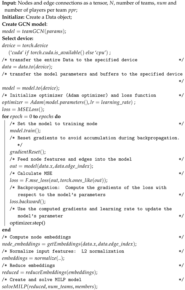
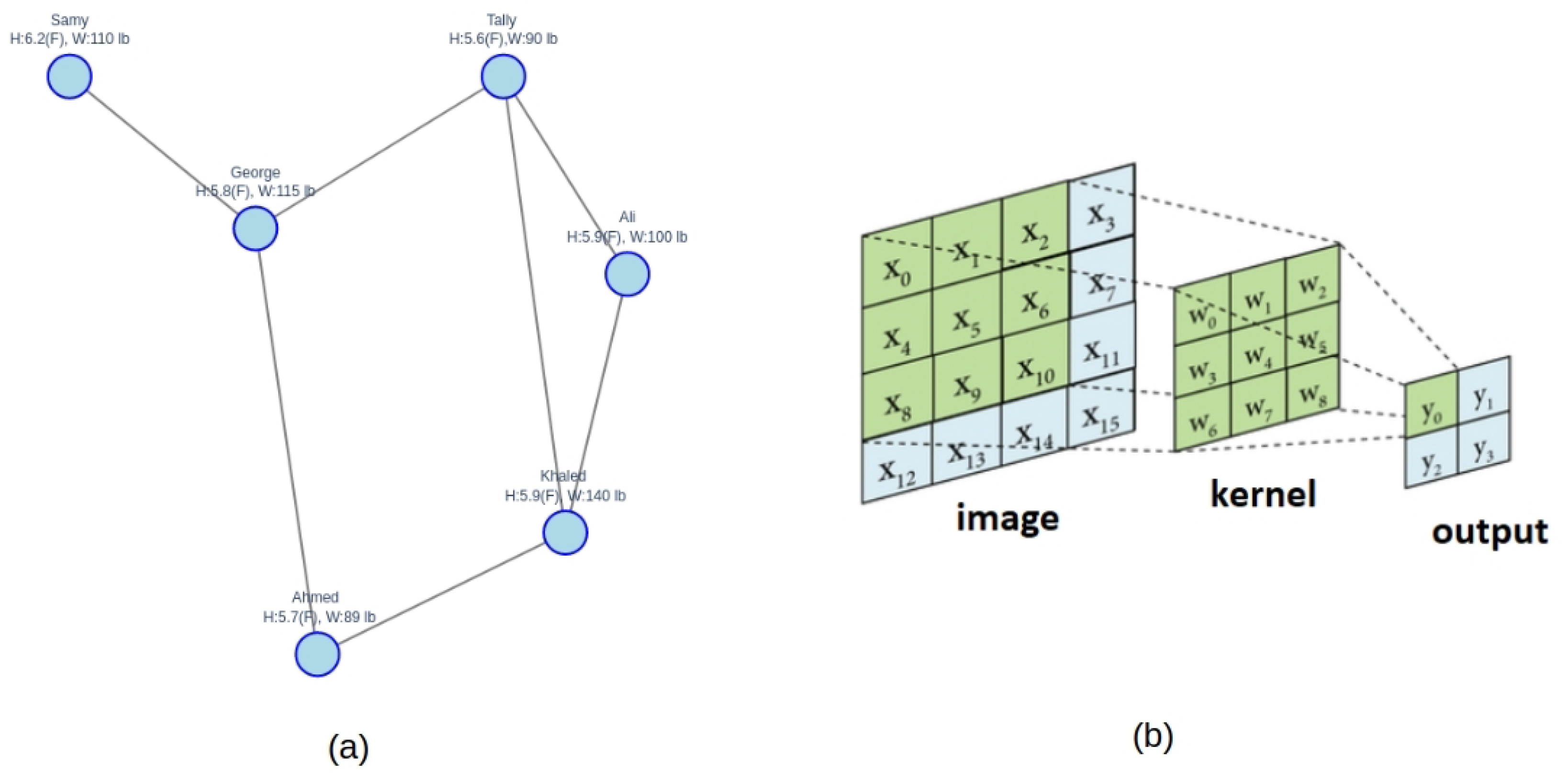
21] further developed and clarified the GNN concept. These early GNN models relied on an iterative message-passing process, where information is exchanged between neighboring nodes until a stable state is reached. However, this iterative approach proved to be computationally expensive. A significant breakthrough came with the introduction of Graph Convolutional Networks (GCNs) by Kipf and Welling in 2016 [
22]. GCNs offer a more efficient way to aggregate information from neighboring nodes, analogous to Convolutional Neural Networks (CNNs) used for image processing. Just as CNNs use kernels to aggregate information from neighboring pixels, GCNs aggregate information from neighboring nodes as shown in
Figure 1. Bronstein et al. [
23] highlighted the importance of adapting neural network architectures to non-Euclidean data structures, such as graph representations, which are particularly suitable for this, citing examples in social networks, molecular chemistry, and gene expression. Although GNNs have shown significant potential in areas such as classification and link prediction, graph clustering remains a challenging task, with existing approaches often struggling to outperform even basic algorithms like K-means; see Tsitsulin [
24].
4. Proposed GCN-MILP Model
In balanced coalitions and teams, we aim at having groups of balanced potentials that are at best equal. While grouping candidates by features might not yield homogeneous teams, we argue that a GNN can provide more accurate approach for the following reasons:
Each candidate is represented as a node with features like skill, experience, position, power, etc.
The GNN can learn rich representations for each candidate by considering their relationships (edges) to other candidates and their individual features (attributes).
We formulate the problem as a clustering problem with constraints. Once the GNN model has learned the node embeddings, clustering algorithms can be applied to group candidates into teams/coalitions. However, we constrain their formation by ensuring that the embeddings among teams/coalitions are as similar as possible to enable as much balance and homogeneity as possible.
4.1. GNN Architecture for the Formation of Balanced Teams
In this work, we consider the graph convolutional network (GCN) to be the most suitable GNN architecture due to its ability to capture the underlying structure of the candidates in the network.
A GCN builds node embeddings by combining information from neighboring nodes. This is shown in Equation (
1).
where
: adjacency matrix with self-loops.
: degree matrix of .
: node embeddings at layer l ().
: learnable weight matrix for layer l.
: activation function (e.g., ReLU).
Next, we explore the components of a GCN needed to solve the TFP:
After obtaining the node embeddings, we have to work around the possible clustering of imbalanced teams. The approach we apply to achieve this goal relies on constraint-based clustering, for which we employ Integer Programming (IP). Therefore, we formulate the last phase of team formation as an IP problem in which we can define several constraints, such as team size, minimum skill level, etc. Thus, constraint propagation and backtracking are necessary to find feasible solutions that satisfy these constraints.
4.2. MILP Model
The main objective function of this model is to minimize the difference in cumulative potential levels between teams, or the DCPLT for short. In order to do this, we introduce the mathematical formulation of the proposed MILP model. First, we define the decision variables.
4.2.1. Decision Variables
4.2.2. Parameters
n: number of players.
m: number of teams.
p: number of players per team.
: skill level of player i.
weighting factor for relative importance.
4.2.3. Objective Function
The objective function is to minimize
while adhering to the following constraints:
where is the required number of teams, is the total number of candidates, denotes the computed candidate embeddings, and represents a two-dimensional matrix of assignment of the size (, ). In the assignment matrix, a cell has a value of one if the candidate is a member of the team or zero if they are not a member. The first constraint represents a validity check that must be satisfied by having each candidate as a member of one team at most. The second constraint verifies that each team has p members at most.
We use PuLP [
25], which includes a default solver algorithm: CBC (COIN-OR Branch-and-Cut) [
26]. PuLP is an open-source solver capable of solving a broad range of LP problems. In addition, PuLP allows for the usage of APIs to enable the usage of other solvers (GUROBI, GLPK, CPLEX, etc.).
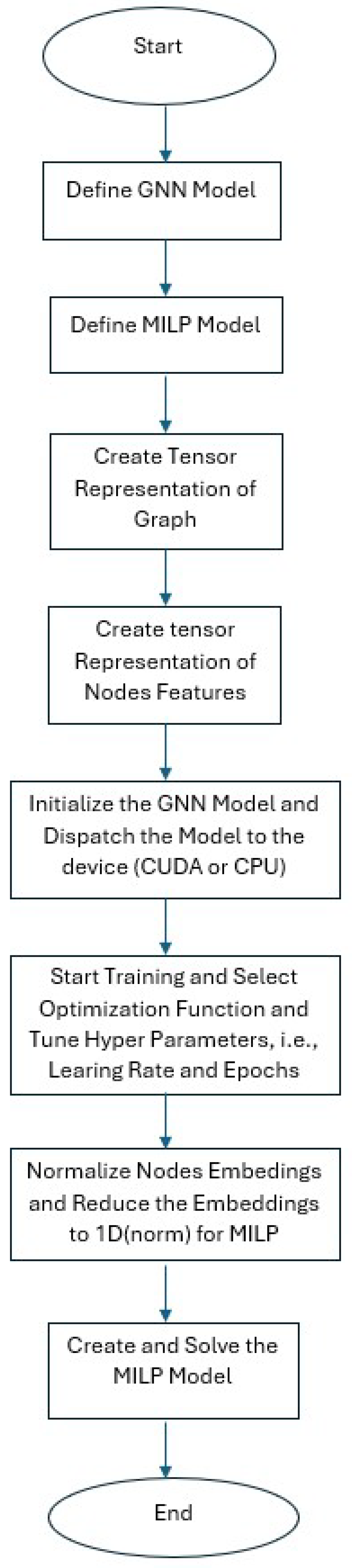
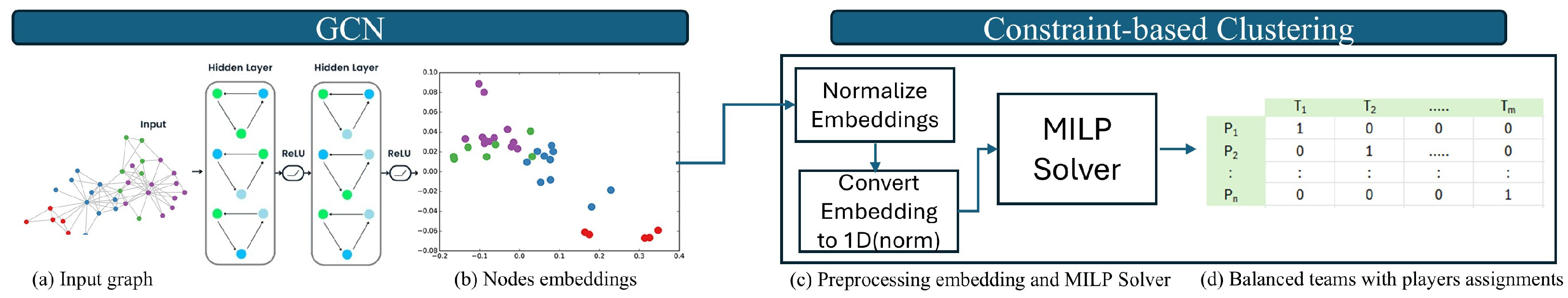
Figure 3 shows the model’s pipeline and the collaboration between the GCN and the MILP solver.
In practice, the systematic adjustment of weights for constraints can be achieved via several methods: iterative refinement, in which one solves the MILP iteratively and adjusts weights based on the results, or a sensitivity analysis, which uses techniques like Pareto optimization to generate a deeper perspective of conflicting objectives, etc. In our experimental work, we employ the technique of iterative refinement as a baseline to test our model.
5. Proposed Balanced Team Formation Algorithm
Generally, we consider the TFP to be a variation of the Set Partition Problem (SPP); see [
27] for more details on the SPP. In addition, the SPP is a variation of the set covering problem (SCP). Also, the set covering problem is considered a constraint programming problem, as all the constraints are 0–1 integer problems; see [
28] for more details on constraint programming. We occasionally use ILP (Integer Linear Programming) to solve the SPP; see [
29] for more details.
Our proposed Algorithm, Algorithm 1, addresses the formulated problem and provides a novel model that takes into account additional constraints. The goal is to create a partition that matches the features of the group members (players). In addition, there are roles that are represented in players’ features and preferences that must be adhered to in order to form balanced teams.
5.1. Experimental Work
For experimental purposes, we have designed a network of fifteen players. Each player has a set of skills represented in vector format. The skills are [‘Attack’, ‘Defense’, ‘Speed’, ‘Stamina’, ‘Teamwork’]. Then, we computed a one-dimensional skill based on weights (preferences) that sums to one, e.g., [0.2, 0.3, 0.1, 0.2, 0.2], as shown in Equation (
8). In this setting, we prefer the defense skill above the others.
To sum up the proposed pipeline from end to end, the workflow fits together as follows:
Input: Graph is represented by an adjacency matrix A and a feature matrix X.
A: matrix, where if there is an edge between node i and node j, otherwise 0.
X: the matrix is the number of features per node.
GCN: Generate node embeddings.
Optimizer: Use embeddings to form balanced teams.
Output: Team assignments and skill balance metrics.
Because the proposed pipeline consists of sequential stages, its overall performance is a direct result of the performance achieved at each stage. Thus, a well-trained GCN is mandatory to ensure the best encoding of the nodes to facilitate the second stage of this pipeline, i.e., the MILP optimizer. In the proposed model, the GCN provides the node embeddings that encapsulate both node features and the graph structure that are input into the optimizer. However, the quality of the embedding is key for several factors: the GCN’s architecture (e.g., number of layers, hidden dimensions), the training process (e.g., loss function, optimization algorithm), and the input graph structure and node features.
| Algorithm 1: GCN-MILP algorithm to solve TFP. |
![Applsci 15 02049 i001]() |
5.2. Experimental Results and Analysis
One of the measures that we employ to gauge the dynamics of the teams and the diversity of the skills that could be required for certain applications is the Gini coefficient, ratio, or index; see Equation (
6). Originally, the Gini ratio was used in economics as an indicator of income equality. Practical results indicate that the lower the Gini ratio, the better the equality. Since we have two factors that are addressed in this work, i.e., team homogeneity and diversity, we can interpret the Gini ratio as follows:
A low Gini ratio indicates that all members of the team have the same skills. This means better homogeneity.
A high Gini ratio indicates that all team members have different skills, which is better when there is a need for different roles within the team. This means better diversity.
where
n represents the number of team members;
and
represent the skills of members
, respectively; and
represents the average skill level of the team.
However, the Gini ratio alone may not provide enough insight into team dynamics. Because of this, we use other complementary metrics, such as the variance of skills within each team, the average skill level per team, and the standard deviation of skills. In addition, some auxiliary plots can help us perceive the distribution of skill across multiple dimensions for each formed team. However, we encountered some limitations in our experimental work due to the adoption of norm-based reduction. While reducing the embedding vectors to 1D can facilitate the use of the MILP model, because this effectively captures the magnitude of the feature vectors and simplifies the computational complexity required, this reduction leads to a loss of directional information, as we only retain the magnitude. To illustrate this idea, we consider the features of three players, as presented in Listing 1.
| Listing 1. Application of L2 Norm on skill vectors |
import numpy. linalg as nl
’ ’ ’
Example embeddings :
(3 players , 5 skill dimensions )
[ Defense , Attack , Stamina , Teamwork , and
Speed ]
’ ’ ’
player _ features = np . array ( [
[ 0 . 8 , 0 . 7 , 0 . 9 , 0 . 8 5 , 0 . 7 ] ,
[ 0 . 6 , 0 . 9 , 0 . 8 , 0 . 7 5 , 0 . 7 ] ,
[ 0 . 7 , 0 . 6 5 , 0 . 8 5 , 0 . 8 , 0 . 7 5 ]
] )
# Compute the L2 Norm for each player
norms = nl . norm( player _ features , axis =1)
# The L2 Norm will look like :
# Expected output
Player norms : [ 1. 7 7 5 5 2 8 0 9
1. 6 9 1 8 9 2 4 3
1. 6 8 4 4 8 8 0 5 ] |
The above feature vectors are replaced by feature norms (e.g., the L2 norm), which are scalar, as shown in Equation (
7).
where
d denotes the feature’s vector dimensions and
i denotes player
i. The resulting player norms shown in the listing clearly reflect the fact that the players’ variations/strengths across the five dimensions dissolved when we opted for the magnitude only. However, simplifying the MILP while retaining some vector information is possible. This can be achieved by using dimensionality reduction techniques, such as principal component analysis (PCA), autoencoders, or weighted norms, as shown in Equation (
8).
However, it is obvious that the L2 norm imposes problems on the TFP, such as not being able to capture different aspects of multiple skills. For example, player
A could be moderately good at multiple skills while player
B could be exceptionally good at one skill, but they may both ultimately have the same norm. This potential situation could hinder the performance of the model. To overcome the potential problems of using the L2 norm in the TFP, principal component analysis can be used as an alternative approach to reducing embeddings to 1D. Thus, principal component analyses can outperform the L2 norm when skills/roles are multidimensional.
The subtle difference between Equations (
7) and (
8) is the emphasis on specific skills over others when forming teams or coalitions.
5.3. Experimental Analysis
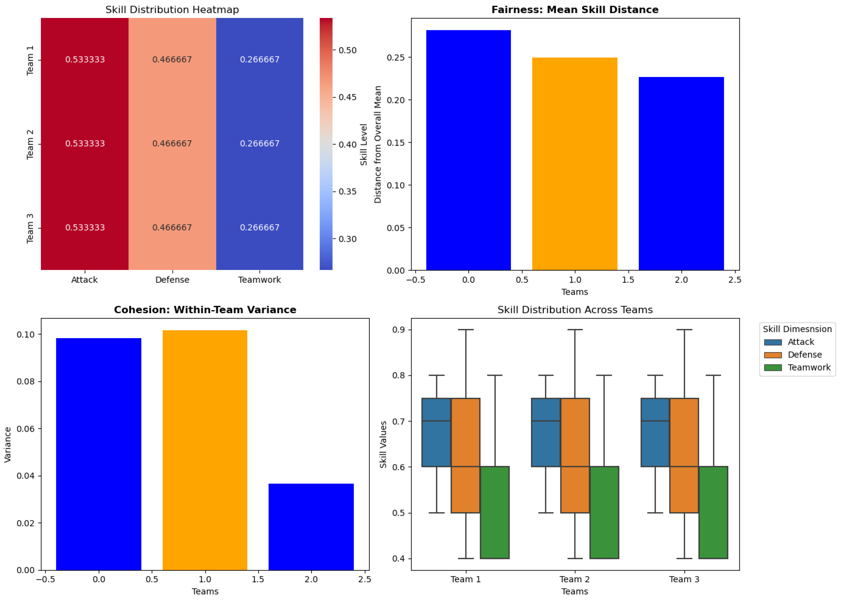
The first experiment that we present has an optimal solution. The first experiment has the settings listed in Listing 2.
| Listing 2. The settings for the first experiment |
# S k i l l s
s k i l l s = [ ’ Attack ’ , ’Defense ’ , ’Teamwork ’ ]
num_players = 9
num_ski l ls = 3
num_teams = 3
s k i l l _ v e c t o r s =[
[ 0 . 7 , 0 . 4 , 0 . 8 0 ] , [ 0 . 7 0 , 0 . 4 0 , 0 . 8 0 ] ,
[0 . 7 0 , 0 . 4 0 , 0 . 8 0 ] , [ 0 . 8 0 , 0 . 6 0 , 0 . 4 0 ] ,
[ 0 . 8 0 , 0 . 6 0 , 0 . 4 0 ] , [ 0 . 8 0 , 0 . 6 0 , 0 . 4 0 ] ,
[ 0 . 5 0 , 0 . 9 0 , 0 . 4 0 ] , [ 0 . 5 0 , 0 . 9 0 , 0 . 4 0 ] ,
[ 0 . 5 0 , 0 . 9 0 , 0 . 4 0 ] ] |
The results shown in
Figure 4 confirm that the teams formed are balanced. The metric “Skill Distribution Heatmap” shows the balance of skills among the three formed teams. Also, the metric “Mean Skill Distance” reflects how the mean skill distance varies slightly among the teams. However, the cohesion metric shows a big variation among the three formed teams. Moreover, we calculated the Gini Coef. and tabulated the results in
Table 1. The Gini ratios demonstrate the homogeneity and equality among teams. The results in
Table 1 indicate that all team members have different skills due to the need for different roles within the team. This could be in favor of diversity and is reflected in their high Gini Coef. of 0.89.
Next, we present a second experiment with the following settings: a pool of twenty players, each with three skills. The objective is to form four teams that each contain five players.
The results of the experiment are shown in
Table 2.
An interpretation of the metrics used:
Mean Skill Distance (MSD): Lower values signify fair skill distribution.
Within-Team Variance (WTV): Lower values signify cohesive teams.
Skill Balance (SB): Lower values signify balanced teams.
First, the MSD score of 0.6222 indicates that individuals are, on average, close to the average skill level of their respective teams. This suggests that the teams formed are homogeneous in terms of their individual skill levels. Second, the WTV score of 1.695 confirms that the teams are fairly homogeneous. Finally, the SB score of 0.1052 is a favorably low value that indicates that the average skill levels among all teams are very similar. Thus, we can deduce that the proposed model successfully generates teams with a balanced distribution of skills.
Next, we introduce a third experiment. In this experiment, we conducted a comparative analysis of our proposed model and two other models: the first was a genetic algorithm, and the second was a modified genetic algorithm with local search and adaptive penalties. The settings of the experiment were as follows: fifty players, each with ten listed skills. The aim was to form five balanced teams.
5.4. Interpretation of the Metrics
A proper interpretation of the results of experiment number three is necessary to understand their relevance to the models’ performance.
First, the mean skill distribution of 0.6222 indicates that the average variation in skill levels between the teams is moderate. Second, the within-team variance of 1.6956 suggests that there is moderate variation in skill levels within the teams. This shows that teams are diverse in terms of skill levels, with a mix of skilled and less skilled players. Third, the skill balance of 0.1052 or 10.52% suggests that the difference between the highest and lowest total skill levels between teams is relatively small compared to the average total skill level. This indicates that the teams formed are fairly balanced in terms of total skills.
Next, we analyze the results of the two models used for comparison purposes, namely the genetic algorithm (GA) and the genetic algorithm with local search and adpative penalties (GA_LS_AP). First, the GA_LS_AP model outperformed the GA in all measures. However, the GA_LS_AP model could not yield teams that were as balanced as those of the GCN-MILP model.
6. Complexity Analysis and Scalability Issues
In this section, we discuss the complexity of the proposed model and its potential computational limitations. The model has two components: a GCN and MILP. The GCN component scales to the size of the graph, while the MILP component struggles with the exponential complexity of large problems.
The computational limitations and the scaling behavior of this model can be decomposed into the following items. First, we discuss its scaling behavior in terms of the following:
Number of Variables: The number of decision variables grows as n (the number of players) multiplied by m (the number of teams).
Number of Constraints: The number of constraints grows linearly with the number of players and the number of teams.
Computational Complexity: The worst case to solve using the MILP in our TFP settings is the exponential one.
Second, we present the computational limitations for large teams, which are as follows:
Memory: MILP solvers need to store the problem’s data, i.e., the search tree generated during the branch-and-bound process. For very large problems, this could be affected by memory limitations.
Solution or Convergence Time: Finding the optimal solution could take a long time when dealing with large problems.
Solver Performance: Some solvers are more efficient than others. Thus, choosing the right solver is crucial. If you have a large-scale problem, Gurobi [
30] and CPLEX [
31] are generally worth investing in, as they are both commercial.
However, some scalability solutions can be used to handle extremely large problems. For example, high-performance computing resources, e.g., parallel computing or cloud computing, might be used to solve the MILP within a reasonable timeframe. In addition, if we are not trying to find the absolute optimal solution and near-optimal or good solutions are suitable, then opting for alternative approaches like heuristics and metaheuristics could be the right choice.
Next, we present a detailed complexity analysis of the proposed GCN-MILP model. The time complexity for the GCN stage is , where l denotes the number of layers, m denotes the number of edges, and signifies the maximum feature dimension across all layers. This relation is computed by considering that the time complexity of each layer is expressed as , where and denote the input and output feature dimensions for that layer, respectively.
If we assume that and are approximately equal and correspond to , the complexity of each layer simplifies to . Then, for l layers, the total time complexity is . The space complexity for GCN is , where n denotes the number of nodes. This space complexity formula accounts for node feature storage () for all nodes; graph adjacency storage (m), needed to store the adjacency information of the graph, which is in a sparse format; and weight matrices for all layers ().
As for MILP, MILP problems are NP-hard, as they grow exponentially with the number of variables and constraints. The worst-case complexity for an MILP problem is , where n is the number of binary variables.
7. Discussion
Using GNNs to better represent relationships and preferences in team formation has the potential to produce a solution that best aligns with the needed quality. The merits introduced by GNN models exceed basic skill-based comparisons. Our approach aims to form balanced teams with a minimization of the variance in skill levels between the teams.
In addition, the utility of the proposed model within the TFP domain is characterized by its extension capabilities. One of the possible extensions that might arise is to ensure the diversity of the teams, in terms of their demographics, personalities, or working styles. This goal can already be achieved by the proposed pipeline (GCN + MILP Solver). First, the GCN is used to encode participant attributes (e.g., demographic, personality traits, working style) into feature vectors. Second, the GCN can learn embeddings that capture participants’ diversity-related attributes based on their connections or features. Third, we can introduce diversity metrics based on the embeddings. For example, if we are looking for demographic diversity, we can measure the distribution of demographic attributes (e.g., gender, age, ethnicity) within each team.
Then, to incorporate diversity into the MILP model, we can either add diversity constraints to the MILP model or add a diversity term to its objective function. For the completeness of this discussion, we will go with one option—adding constraints—to check whether this model can meet a diversity requirement (i.e., demographic balance). First, we need to ensure that each team has a balanced representation of different demographic groups. Then, we introduce a binary indicator
, where
if player
i belongs to demographic group
g, and 0 otherwise. Second, we add constraints to ensure that each team
j has at least
and at most
players from group
g:
Furthermore, we can argue in favor of team formation under the condition of unbalanced skill distributions. This is achievable if we neutralize the effect of the term . This could be achieved by setting . The effect of removing the balance objective would be a highly skewed distribution.
Moreover, possible extensions of the model to handle more sophisticated constraints to create more controllable team formations are feasible and can be achieved through several approaches. The first approach is a shift from skill balance to providing a certain upper and lower bound for the skill level per team. This is achieved by adding the following two constraints:
The second approach avoids placing two players in the same team due to aversion or a lack of chemistry. For example, player
and player
cannot be on the same team. As such, a new constraint is added, which is as follows:
In addition, other metrics may be investigated, for example, the within-cluster sum of squares (WCSS), Silhouette Coefficient (SC), Davies–Bouldin Index, etc. However, these metrics need to be adapted to fit the context of our specific team formation model.
8. Conclusions and Future Work
Graph neural networks have shown flexibility in understanding the relationships between entities, incorporating preferences and learning complex interactions between domain-specific nodes. Using graph convolution networks (GCNs) to address the team formation problem offers the advantages of flexibility and adaptability in terms of their ability to reflect network dynamics and relationships. In this work, we propose a hybrid GCN and MILP model to solve the team formation problem. Based on experimental work, the proposed model is capable of obtaining the optimal solution if it exists. A possible shift to heuristic, metaheuristic, or greedy approaches could provide a near-optimal solution in a reasonable amount of time, even if these approaches are not guaranteed to provide the optimal solution. Future work may investigate graph attention networks (GATs), leveraging their attention mechanism for enhanced feature learning and dynamic weighting. This mechanism, along with GATs’ ability to model diverse node relationships and incorporate inductive bias, also contributes to greater interoperability and flexibility. In addition, GATs use attention mechanisms to weight different nodes differently (heterophily). However, close attention must be paid to the increased computational cost of GATs.


