An Artificial Intelligence-Based Digital Twin Approach for Rejection Rate and Mechanical Property Improvement in an Investment Casting Plant

Abstract

The manufacturing process carried out in the investment casting industry suffers from problems similar to other production processes. In addition, the high requirements of the customers and the industries that require these parts mean that high quality standards must be met. If those requirements are not achieved, this leads to the rejection of the manufactured parts. Therefore, given the current technology revolution (i.e., Industry 4.0) and the possibilities offered by tools such as digital twins and artificial intelligence, it is possible to work on a generation of intelligent systems that can reduce and even avoid these problems. Therefore, this study proposes the creation of a digital twin based on artificial intelligence to work on proactively identifying problems before they happen and, if they are detected, launch an optimization process that offers corrective actions to solve them. More specifically, this work focuses on the analysis of the manufacturing process (definition, KPI extraction, capture, distribution, and visualization), the creation of a base system for the integral management of process optimization, and experiments developed for determining the best method for making predictions. Additionally, we propose a recommender system to (i) avoid the appearance of porosities and (ii) keep the elongation of the parts in the ranges desired by the customer.

1. Introduction

Society has been evolving for years and increasing its population; thus, the demand for products is increasing. Specifically, many products need metal parts produced by the metalworking industry, which has evolved since the different metal ages in human history [1]. In order to make this type of production feasible, the industry realized that it must improve and optimize its production process. Currently, there are a large number of foundries that employ different production methods. For instance, there are foundries that work with green molding, chemical molding, or shell molding, among others. This type of manufacturing process dates back to ancient metalworking eras. In contrast, investment casting, although not widely adopted, is an industry with very high demand due to it being able to generate very sophisticated parts. As a result, it is a complex and expensive process.

The investment casting process was created thousands of years ago in the Chinese empire. The main characteristic of this process is the possibility of creating very precise castings with difficult geometries to fill. Moreover, it is able to use a wide range of metallic alloys for manufacturing its parts compared with most popular foundry processes. Hence, this process is suitable for high added value and small series of highly demanding parts [2]. The main sectors addressed by this process are the aeronautic, automotive, and weapon-making. These types of industry are final users that require an additional degree of safety of their products [3].

These manufacturing processes, because of their nature, have a common challenge. They are very sensitive to variables related to the ceramic mold building up around the wax pattern, to the melting and pouring conditions, and in some cases, to the final heat treatment. In this way, the main problem is the presence of different defects on the final parts, like shrinkages and pores that require re-fixing of the component or even its final rejection [4]. Another problem is the process itself. The part is only visible at the end of the process, once finishing operations have been carried out. At that point, if problems are discovered, they are converted into significant loses to companies as non-quality costs. The most common strategy to address this problem is to understand the behavior of the process by developing process simulations based on physics concepts like fluid dynamics and heat transfer. These models are focused on forecasting the final performance of produced parts based on variables like the filling speed, heat transfer, and contraction during solidification. They can make predictions in terms of slag formation, shrinkage, or hot cracks, respectively. This kind of task makes the manufactured part more expensive. In addition, castings are affected by a variety of different factors; for example, the metal composition, mold design, and casting conditions, which can influence the final outcome [5].

Currently, the industry is seeking alternatives to avoid part defects [6], providing solutions that can predict the soundness of the parts. Moreover, during the last decade, significant effort was dedicated to improving final product quality, supported by the use of ICT, its integration into manufacturing equipment, and the application of the internet of things.

For example, Dučić et al. [7] reviewed several studies in the literature that make use of artificial intelligence (AI) models to improve parts or processes. Thus, the authors collected information regarding several types of manufacturing processes; for example, sand processes and continuous processes, among others. They also discussed investment casting, describing how ANNs have been used to perform numerical simulations of different mold temperatures [8]. More accurately, they work to manage some aspects such as mold temperature, melting temperature, casting part material, number and location of feeding points, diameter and length of inflow channels, and the angle of the channel with respect to the main sprue axis. Similarly, Pattnaik et al. presented how to optimize the injection process parameters with multiple performance features in the investment casting process using an orthogonal array with gray fuzzy logic. This algorithm identifies an optimal combination of the process parameters [9]. Moreover, recent studies utilize modern techniques such as advanced deep learning models to carry out visual inspections of parts [10]. In this case, the defect has already been produced. This means that this approach does not work proactively, but it shows how AI techniques can be used in various ways to improve the manufacturing process.

The arrival of Industry 4.0 [11] has significantly accelerated efforts to optimize the manufacturing process. Specifically, this kind of work requires digitization of foundry plants, driven by the improved data-gathering capabilities of machinery. Therefore, as a result of ICT advances, different studies have been carried out which use these data as the basis for new systems [12]. For example, ref. [13] presents a data-driven framework based on machine learning techniques for estimating and screening early products in investment casting. Additionally, digital twin technology has significantly contributed to improving manufacturing processes. For instance, Antoniadou et al. focused its research on handling the robots that manage the investment casting molding stages [14]. This kind of tools were also used for checking and detecting defects like deformations [15] and stress [16] in aeronautics parts. Finally, a research paper was presented in the 75th World Foundry Congress (WFC) that presents a digital twin for porosity detection [17], but without checking the best optimization parameters to avoid pores.

Against this background, we try to combine these ICT technologies and ideas for process optimization. We generate a digital twin that is able to observe the manufacturing process, extract the current situation, predict the possible further $t+1$ stationary state, and, when anomalies are detected, provide corrective actions to avoid them. This is similar to Model Predictive Control (MPC) systems [18].

To achieve efficient digitization of an industrial process, several steps were carried out. In this way, this research started from a digital audit evaluating process traceability, frequency, and precision of the controls. Also, digitization analysis of existing data, preprocessing possibilities, and visualization was performed. Later, capture agents were developed to preprocess and store data in a central and ordered database. Moreover, we continued providing access to extracted information and generating different query methods to detect deviations and trends. Next, we built a digital twin, a virtual representation of the process, and we provided it with the tools to identify interconnections between variables and product output characteristics through an advanced data analytics process. Finally, the generation of predictive algorithms to foresee the expected characteristics of the manufactured parts and a recommender system to ensure final results were implemented and included in the final system. For this research, we focused on two defects: (i) mechanical properties and (ii) rejection rate.

The remainder of this paper is organized as follows. Section 2 describes the work and the steps undertaken to achieve the proposed solution. Additionally, this section discusses data generation, the methodology, and the development of the intelligent system. Section 3 presents the results achieved with the proposed approach. Here, we introduce the generated results for several configurations, as well as the final solution created for investment casting. Finally, Section 4 concludes this paper and the research, providing a discussion of the solution and suggesting future work and potential improvements to our proposal.

2. Materials and Methods

Therefore, in an attempt to solve the already defined problem in Section 1, as well as the difficulty of addressing the process as a whole, researchers have proposed the use of the well-known “Divide and Conquer” (divide et impera) methodology. More accurately, this methodology tries to divide the general problem into smaller ones. In other words, it tries to transform the original problem into simpler ones that are easier to solve. Thus, once a solution has been found to solve each of them, the combination of all achieved developments solves the general problem. This methodology is widely used to deal with legal challenges [19], mathematical calculations [20], and computational problems (specifically in parallel processing) [21].

Consequently, building on this idea, the steps defined in this work are detailed below (additional information is shown in Figure 1).

• Identification of the problem and the challenges to overcome: The goal of this initial step is to identify the background and context of the original problem. In essence, we focus on gaining a clear understanding of what we are aiming to solve.
• Acquisition of knowledge: Collecting high-level knowledge provides the necessary overview to start the research. Nevertheless, later, when we focus on a more specific aspect of this challenge, this step will be repeated to ensure greater accuracy in the new generation of specific domain solutions.
• Division of challenges: Starting from the idea of divisions mentioned earlier, we will define the challenges to address and the specific steps for each one. For this research, the following challenges have been identified: (i) digitization and manufacturing process representation, (ii) creation of a proactive system based on predictions, and (iii) retro-feedback for controlling and adjusting the manufacturing parameters. For each of them, the following sub-phases will be performed:

  a

  Acquisition of specific knowledge: Once the topic is defined, this stage involves expanding the knowledge necessary to address the problem. Frequently, this knowledge acquisition is closely linked to the exploration and understanding of the production process being optimized.

  b

  Definition of the experiment and the techniques to be used: At this point, the specific research and experiments are outlined for each of the challenges to be addressed.

  c

  Evaluation: At this stage, the defined experiments are conducted, and results are obtained for the approximation that has been defined.

  d

  Analysis: Once the previous stage is complete, the collected data from the experiments are analyzed.

  e

  Interpretation of the results: When each solution has been determined for all identified challenges, we will combine them.

Any type of optimization of the manufacturing process, such as the manufacturing of castings using an investment casting process, involves exhaustive control of all associated operations. The more control there is and the fewer fluctuations that occur, the more reliable the results of the process. In this manner, the optimization and stabilization of the entire manufacturing process must be supported by Information and Communication Technologies (ICT). Thus, according to Boscher et al. [22], the main goals are as follows:

• Digitization of the process: It is fundamental and necessary to digitally represent the manufacturing process.
• Expand the amount of digitized information, achieving a representative set that facilitates the understanding and management of the process.
• Generate a robust IIoT (Industrial Internet of Things) system designed to correctly define the appropriate ICT solution.
• Provide a solution that, in addition to describing the current behavior, can provide digitally calculated solutions that improve the real system.

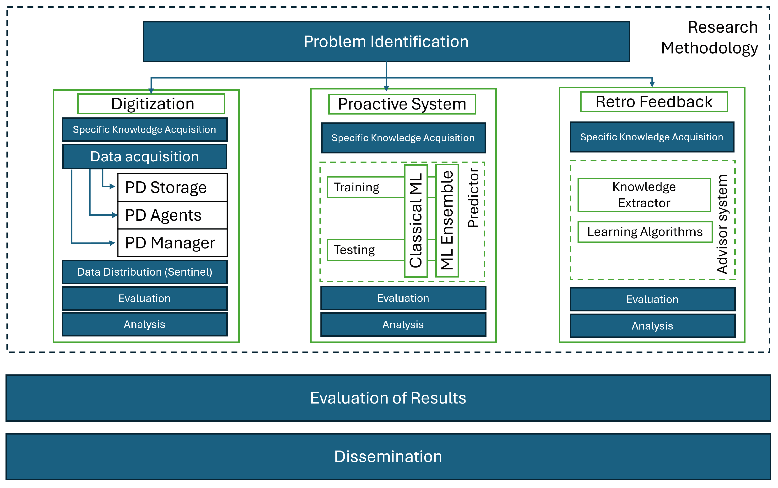
Consequently, after applying the aforementioned methodology and the main goals described by Boscher et al., the global proposed solution is defined as a System of Systems (SoS) comprising an agent-based data gathering architecture for creating a complete manufacturing process digital twin. This system focuses on detecting anomalies through predictions and, finally, an advisory system to redirect the process to normality.

2.1. Digitization and Manufacturing Process Representation

As defined in [23], a system is a collection of interconnected elements that, when combined, produce results unattainable by the elements operating independently. These elements can be complex and large in scale, consisting of sub-elements working together to achieve a common objective.

The concept of a system of systems refers to a scenario in which the constituent elements are themselves collaborative systems, each exhibiting the characteristic of operational independence. In particular, each individual system can achieve a functional purpose independently, without relying on its involvement in the broader system of systems. Furthermore, each system maintains managerial autonomy, meaning it is managed and evolves to fulfill its own goals rather than those of the overarching system [24]. As discussed by [25,26], these attributes distinguish a system of systems from large monolithic systems. Fields such as enterprise architecture and service-oriented architecture address systems with these defining features, enabling the development of such solutions.

The architecture of a system is critical to its success in meeting the objectives of its stakeholders [27]. In this case, it is defined as the collection of structures necessary to understand the system, including its components, the relationships between these components, and their properties.

In light of this explanation, the general sub-challenge addressed in this research is to create different individual systems for data collection to build the digital representation of the process. Each system can operate independently and solve the acquisition problem within its own area or domain. Moreover, all of these modules are designed with the necessary communication capabilities to interact and carry out their specific tasks toward achieving the final objective: the optimization of the production process as a whole.

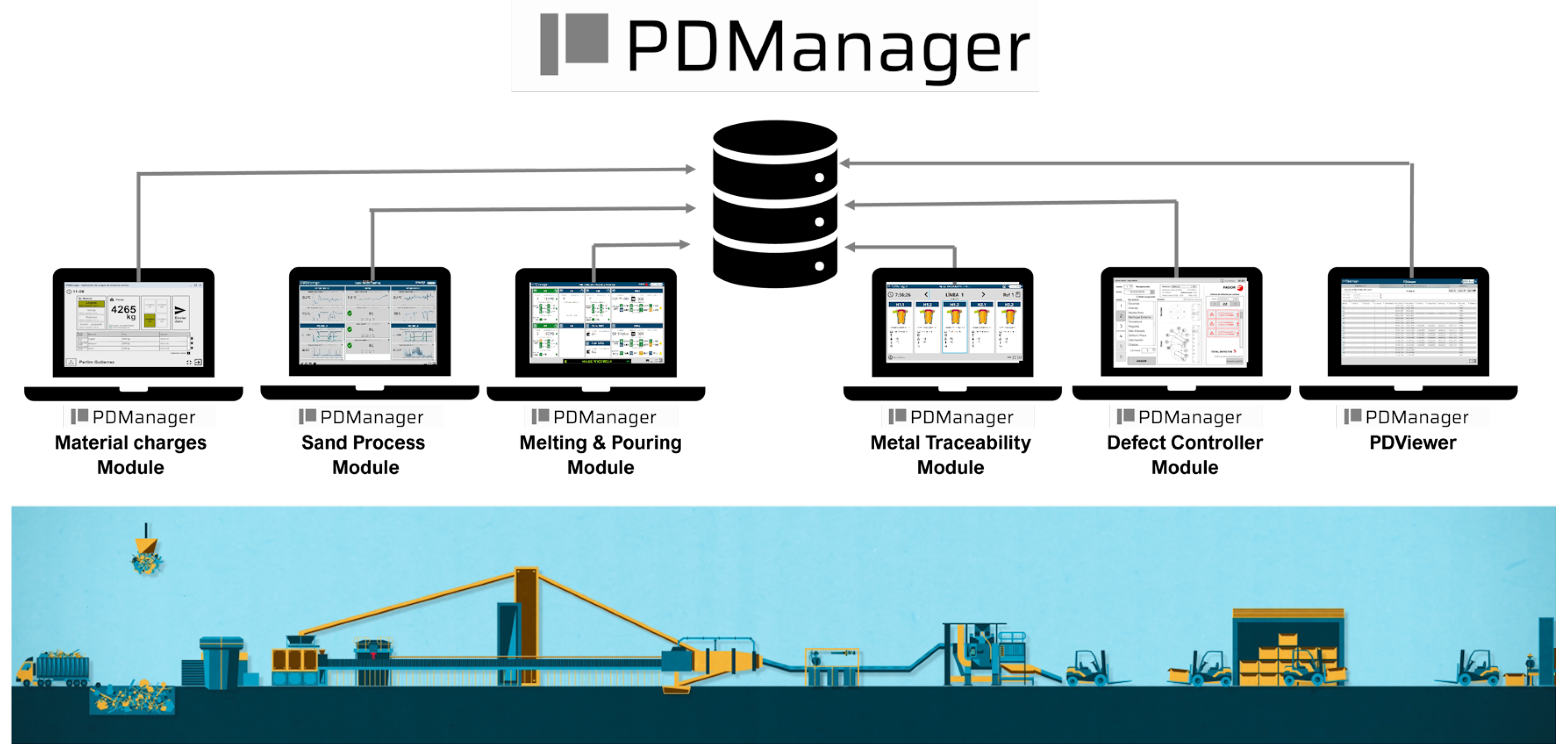
To carry out this data gathering process, the Production Data Manager tool, PDManager, developed by the Azterlan Research Center is used (for more information, please visit https://www.azterlan.es/en/kh/pdmanager, accessed on 20 January 2025). Specifically, PDManager is a real-time production control system designed to guarantee digitization, traceability, and the orderly storage of key parameters in a centralized database for the manufacturing process of cast components.

This system is composed of three root elements:

• PDStorage: A centralized relational database where all the gathered data are correlated, keeping the production history. In addition to being used for monitoring and recording information in real time, it can be employed for knowledge generation and predictive model creation based on these provided data. This kind of storage system and its capability to centralize data and information is discussed in the literature [28,29].
• PDAgents: Small software artifacts created as services that focus on the specific task of interacting with third-party entities (i.e., other databases, files, or even machinery), extracting the necessary data from the production process itself. Krivic et al showed in [30] how these developments can create the needed data flowing ecosystem for IoT management. The creation of this type of micro-service is the axis of a more complex software architecture that can also help in other domains like smart agriculture [31].
• PDManager modules: The PDManager system has different modules (some of which can be seen in Figure 2) that, first, allow the operator to interact with and monitor the area where they are located and, second, provide a tool to perform manual correlation of data when automatic correlation is not possible.

Regarding the process explanation given in Section 1, to address the aforementioned management process, data must be extracted from the entire manufacturing process. The deployment of PDManager focuses on implementing different modules that manage the following process areas: (i) primary coatings, (ii) secondary coatings, (iii) melting, and (iv) final inspections.

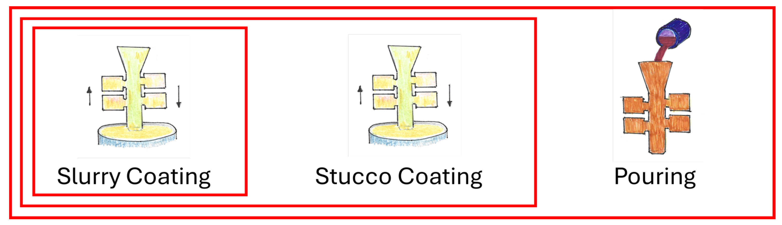
Specifically, the first stage of data aggregation relates to the coating process. In detail, the primary coating is the phase where the first layer of wax is applied to the model. Its primary purpose is to create the model’s surface. To achieve this, a liquid suspension, also known as slurry, is used. The slurry consists of a fine ceramic material and a binder with high heat resistance and good adhesion. Subsequently, the secondary coating involves applying additional layers on top of the primary layer. Its main function is to provide mechanical strength and structural stability to the mold. Therefore, coarser sand is used together with a colloidal silica binder.

The addition of each coating, which will eventually be converted into a shell mold, is of great importance. For primary and secondary coatings, the data to be captured are the environmental data for the room, which are obtained from a third-party platform provided by EKIOM^TM company from Paris, France (https://www.ekiom.net/, accessed on 20 January 2025). EKIOM^TM records temperature and humidity data with different sensors placed in the primary and secondary areas. In addition, slurry data are extracted from the pre-existing Factory Win platform deployed in the foundry. This information is supplied by a Microsoft^TM Excel^TM file located in the coatings laboratory. This document compiles data related to slurry analyses carried out periodically through rigorous internal procedures in the foundry. More specifically, the variables include density, temperature, SiO₂ percentage, and others.

These parameters are critical because if the environmental data are not correct, the mold layers will not dry under optimal conditions, causing mold breaks. Furthermore, if the slurry creation is incorrect, it will cause poor adhesion between layers, which may also cause mold breakages.

Then, in the melting area, the controlled data include the chemical composition of the alloy, the temperature of the furnace, and other variables related to the casting. At this stage, the data flow in two different ways. On the one hand, some data are manually digitized through the PDManager Melting and Pouring module. On the other hand, several pieces of data are stored in the Factory Win platform and are automatically detected and extracted from it. Specifically, composition data are measured via spark spectrometry analysis performed in the chemical laboratory, while the rest of the data are generated by various sensors connected to the corresponding equipment.

For the last area, the final inspection, the gathered information pertains to the quality results of the manufactured castings. The data focus on the occurrence of shrinkages and mechanical properties, such as elongation, which are analyzed in this research. For this last data extraction process, information about inclusions is obtained from PDManager, which is connected to Factory Win and continuously updated with results from fluorescent particle tests performed on all created parts. This process is carried out by qualified technicians who determine the number of pores/inclusions in each part. Additionally, elongation data for castings are provided. For this purpose, representative standard specimens from the manufacturing order are machined and later tested to obtain the final mechanical properties, which are then digitized via PDManager.

Once the data are extracted and stored in the appropriate repository, they should be utilized to improve the day-to-day process. Thus, they will be used to represent the production process, delivering the right information to the right people at the right time. The most effective way to achieve the goal of data distribution is by implementing an observer/observable pattern [32], which is based on the subscriber/publisher paradigm [33].

During the past decade, communication schemes have been redesigned and reimplemented with the aim of integrating data from several heterogeneous data sources. Moreover, the introduction of certain standards (for instance, the IEC 61850 standard for substation automation [34]), which defines a data model oriented toward objects and functions, allows for modeling all the devices of a system by categorizing them according to their functionalities. This technology also enables their integration into a high-speed peer-to-peer communication network through standardization. However, further improvements were needed to establish an open and standardized working environment. The solution was the creation of a real-time publisher/subscriber communication model, as demonstrated in [35]. In fact, this type of communication is widely used and well documented in books and research papers such as the following: [33,36,37,38].

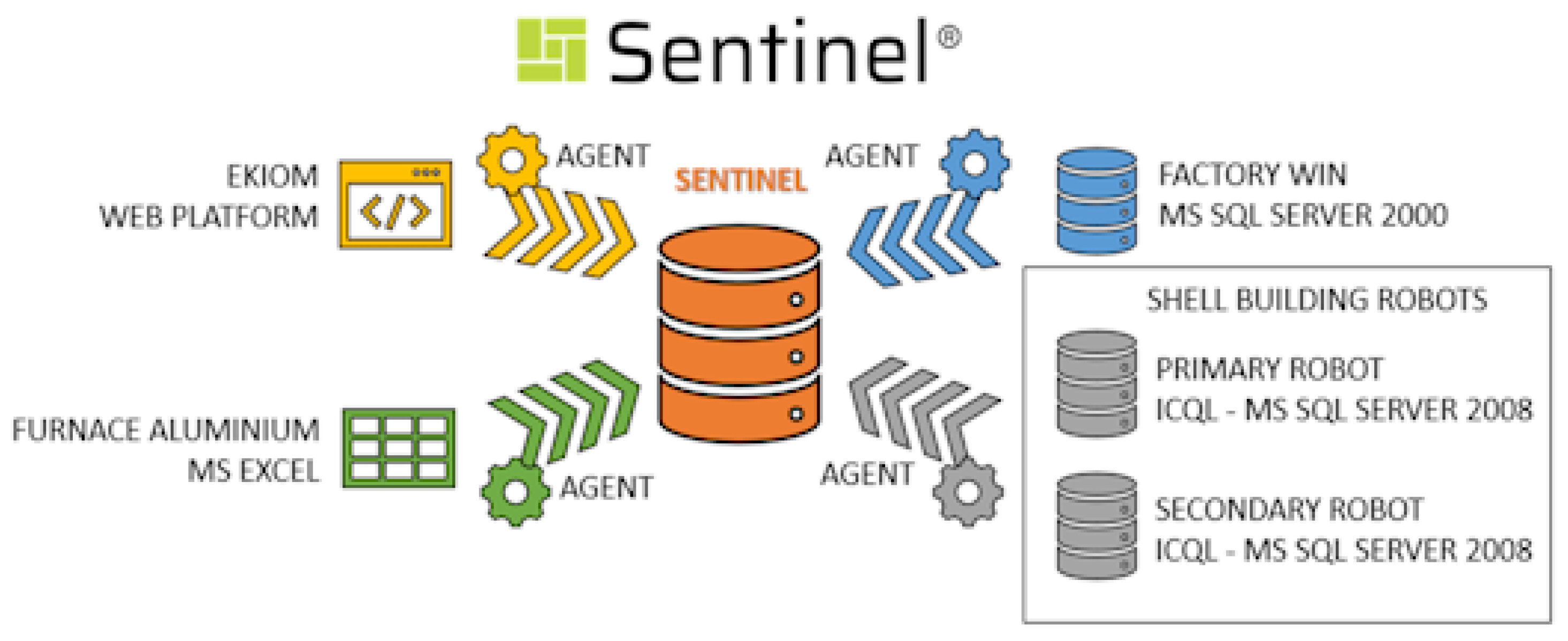
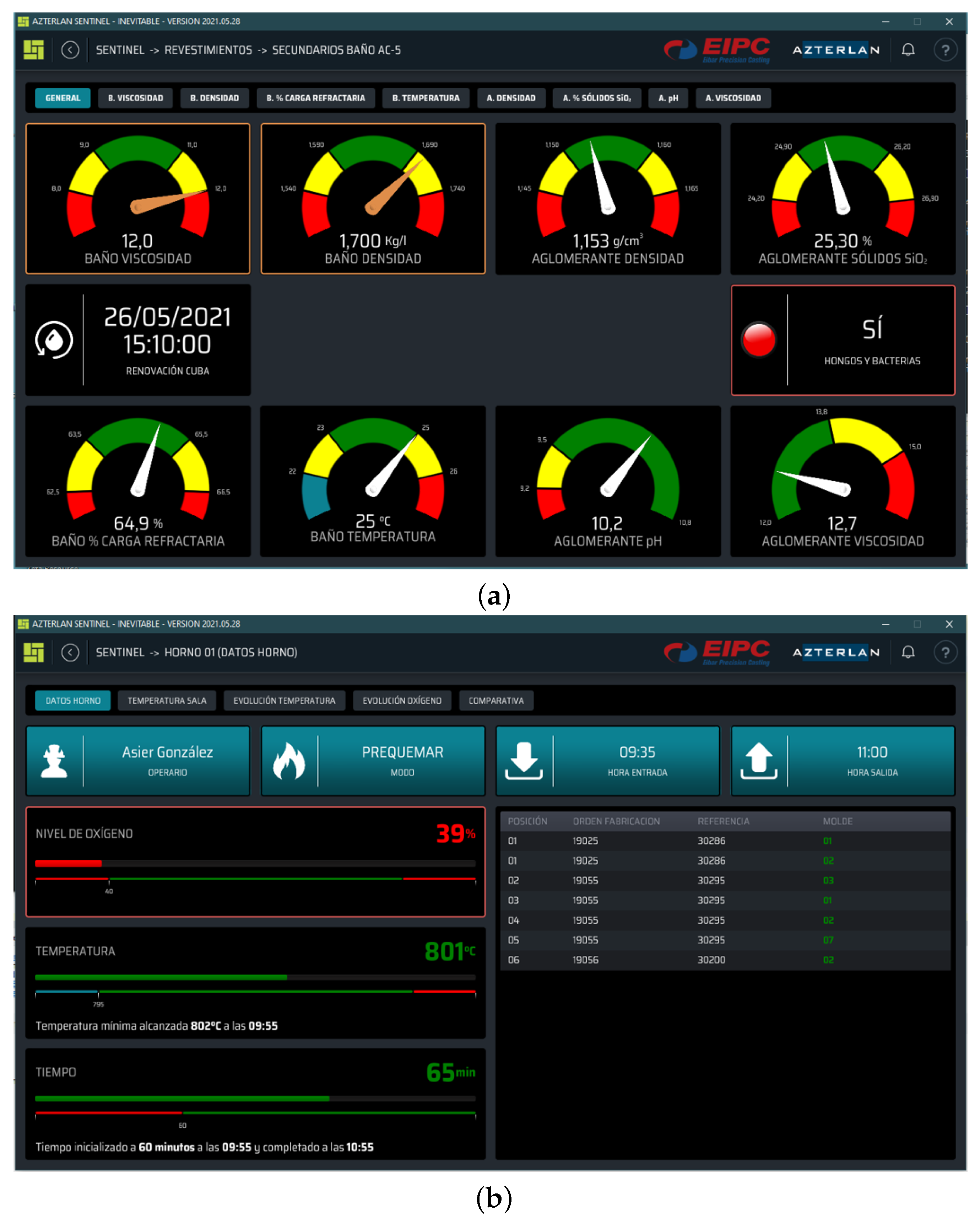
In a effort to combine this communication and data distribution technologies, Azterlan developed Sentinel (for more information about Sentinel, please visit https://www.azterlan.es/en/kh/sentinel-predictive-control, accessed on 20 January 2025). It is an integral system for data distribution and process monitoring, as well as anomaly detection, digital representations of the process, alert communication, and a tool for incorporating and utilizing different Artificial Intelligence (AI) models. 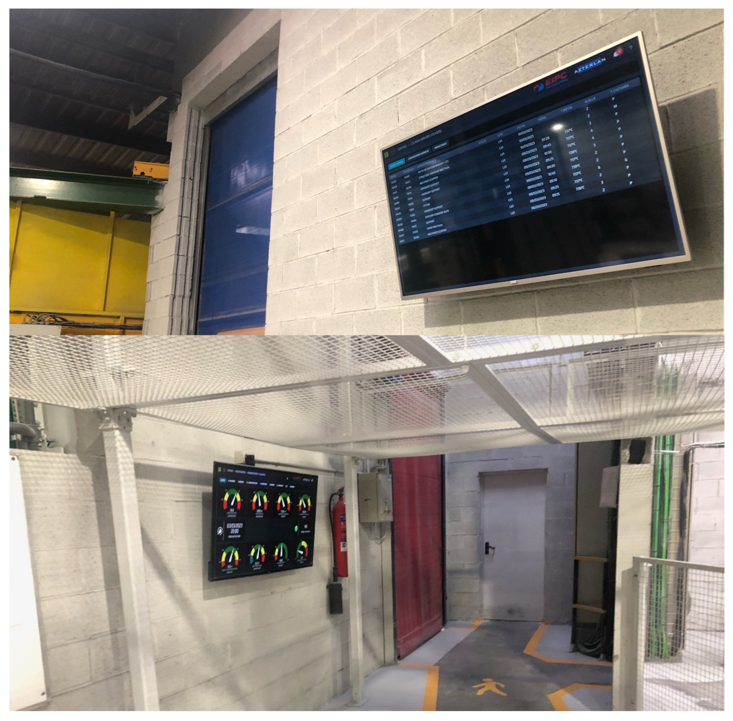Despite all the features available in the Sentinel system (illustrated in Figure 3), at this stage of development, Sentinel is focused solely on distributing, displaying, and presenting the gathered information. Hence, for now, we define Sentinel as a software system for automated and real-time data distribution. Sentinel displays key information and alerts to the people and locations where they are most useful. It allows for the deployment of dashboards or control panels designed according to user needs. These control panels can be implemented as static displays (on-site) or with navigation capabilities across different levels of information depth (e.g., process managers, laboratory, quality department, maintenance, and management, among others).

In order to define and design the data distribution, as well as the visualization methods in Sentinel, the following aspects have been analyzed:

• KPI identification: Firstly, the work team determines the key process indicators that are valuable for the day-to-day work and the management of the process. In this way, the different areas that can be included and the different data that can be employed are studied here.
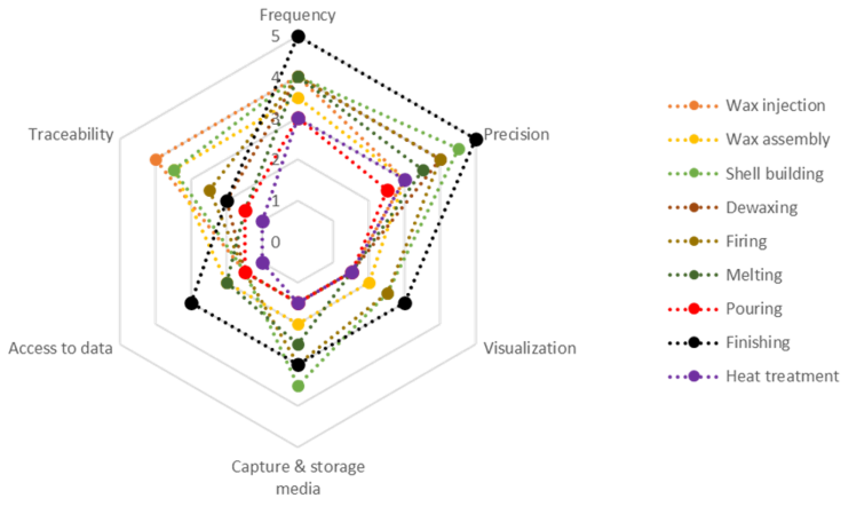
• KPI analysis: Once the interests and possibilities were listed, we developed an analysis addressing all key stages of the process. To achieve this, six different variables were compared using the Likert scale [39] and combined in a Star Plot. The variables used are: (i) frequency, (ii) accuracy of the available information, (iii) visualization or its necessity, (iv) capture and storage media, (v) possibility of data access, and (vi) traceability.
• KPI Priority. After the previously conducted study, a filtering process is developed based on the priority of working on these indicators. This analysis is performed using a scatterplot.
• Data distribution location. As the final task, the appropriate location for each visualization is determined.

In the end, the management of all input sources was performed, as shown in Figure 4. Four different PDManager capture agents were developed to integrate these data sources. Subsequently, all the information was centralized in a single database, allowing Sentinel to utilize it for data distribution and visualization in this specific use case.

2.2. Creation of a Proactive System Based on Predictions

Thanks to the work defined and described in Section 2.1, we now have all relevant process information available. This information flows in real time through our capture and storage system. Hence, all the described data serve as the raw input necessary to create an intelligent process management system. The collected data enable the digital representation of the process using advanced techniques. In fact, these data allow us to develop a proactive intelligent system that anticipates potential problems in the process. Its creation will be carried out through what is known as a digital twin.

More accurately, the concept of a digital twin [40] refers to the creation of a virtual and intangible representation based on real data. Its objective is to replicate a physical or real situation. In our case, it focuses on representing the investment casting manufacturing process. The main contribution of a digital twin is to decouple the physical world from the virtual one, enabling analysis of how the process operates and subsequently preventing unexpected deviations in both virtual and real representations.

For our use case, the digital twin must facilitate process improvements aimed at defect reduction, energy efficiency, and time-to-market reduction. To achieve these objectives, the digital twin must operate under three clear axioms, as well defined in [41]:

• Proactivity: The system must be able to anticipate adverse situations. In fact, the digital twin makes use of the digital world through simulations and artificial intelligence. Thus, it will be able to determine the possible state of the production process in the near future (i.e., a temporary state $t+1$).
• Adjustment: The management of the virtual environment must always work within a specific configuration. This means that the digital twin must meet the requirements of the manufacturing process. In other words, none of the tests or simulations that are developed will break the rules that govern the physical representation of the process.
• Business intelligence: The twin will even serve as a knowledge management tool. Specifically, it is a repository of business intelligence that encompasses everything needed to manage all the tasks associated with the actual process. By utilizing the digital twin and providing it with this repository, business knowledge will remain within the company, preventing the much-feared knowledge leakage.
  For a digital twin to work, it must apply the same methodology that a doctor does. This methodology is called “diagnosis”, and its basic steps are as follows [22]:

  (i)

  Observation: The digital twin is based on observation, which serves as the foundation for the digital representation of the real world. Observation focuses on extracting raw data, as previously explained and defined. This observation is essential because it enables the identification of operational patterns, trends, and other aspects that will be used in subsequent tasks. It is important to note that without observation—in other words, without a data capture process—developing this type of technology would not be possible.

  (ii)

  Evaluation: Making use of the knowledge already loaded into the twin, as well as the data that are being produced in real time, our system develops a process known as “evaluation”. This process performs different simulations based on the current real situation it receives through “observation”. Subsequently, the further operations required to adjust and optimize the process will depend on the evaluations or predictions obtained in this stage.

  (iii)

  Decision making: The previous processes, by themselves, do not add value. That is why a correction or adjustment of the monitored activity is needed. Thus, taking into account the results of the observation and evaluation steps, solver algorithms find the appropriate fit for the purpose of the twin. Afterwards, the system proceeds to communicate the results or actions that must be put into practice [42]. Sometimes, they are sent to humans (M2H–machine to human communication), and other times, they are sent to machines via M2M (machine to machine).

In order to generate a tool capable of representing the reality of the manufacturing process, specifically, the production of molds and parts flowing in the investment casting workflow, it is necessary to be able to represent the flow of these molds in the lost wax casting process and the events that occur in it. In this case, the data obtained from the primary coating, secondary coating, melting, and inspection areas will be transformed into a sequence of enqueued elements that are sequentially characterized in each stage and digitally represented as a FIFO queue.

Hence, our digital twin was formally defined as a queue Q of z discrete molds, where V is the sum of $PC+SC+M+I$ molds ($PC$ for primary coating and previous molds, $SC$ from primary coating to secondary coating, M from secondary coating to melting, and I for final inspections). Some variables will not be informed until the mold arrives at the specific stage where that data are gathered. In the end, the entire representation is defined as $Q{x}_n,\dots ,x_2,x_1\to Vp{c}_n,\dots ,p{c}_2,p{c}_1,s{c}_n,\dots ,s{c}_2,s{c}_1,m_n,\dots ,m_2,m_1,i_n,\dots ,i_2,i_1$. For our use case, $\left|V\right|=40\to \left|PC\right|=\left|SC1\right|=\left|M1\right|=\left|I1\right|=10$, and when the full set of $PC$ molds is ready, they are all moved together to the next step, pushing them forward in the $PC\to SC\to M\to I$ sequence.

In order to reproduce the current situation of the process, the digital twin must be able to model the movements of the molds, as explained before. In this way, it performs event-based management of the system, detecting when a group of molds reaches a new sequential step, represented by each red square in Figure 5. In fact, the digital twin operates under the following events:

• The first event occurs when a set of molds is being generated in the primary coating stage. To detect this, the digital twin is subscribed to the PDManager storage database. During the coating process, the system collects data until the last coating has dried and the robot moves the mold to the next stage. When the full set of molds is completed, the digital twin receives this event from the database and triggers a series of tasks to digitally generate the process state, update the digital twin, perform the associated calculations, and finally, move these molds to the next step.
• The second event is triggered when the secondary coating is applied. The digital twin is again subscribed to the storage, and the event is fired to indicate that some work must be performed. This second event functions similarly to the previous one but pertains to the creation of the final mold. Again, when all molds are created, the digital representation is updated, and all calculations are executed. Finally, the entire set of molds is promoted to the next stage.
• The last detected event occurs when the casting is finally created. This means that the final event is fired when the metal is poured into the mold. Again, the system operates in batches of molds. The subscription to the PDManager database triggers the management process for this step. At that moment, the digital twin receives the information about the creation of the castings, and all of them are moved to the final steps. These last steps are not monitored in this research, though they could be incorporated in future developments. Nevertheless, after the completion of the castings, the quality of each casting is measured, and these data are gathered for the prediction methods. While this is not a step for the digital twin, it is crucial for anticipating the behavior of each casting concerning mechanical properties and the appearance of porosity.

Due to these events and the data gathering process, the digital twin is able to characterize each mold. At this moment, the mold $V_j$ has the set of variables $P{C}_i,S{C}_i,M_i,I_i$ that can now be sent to the machine learning models, which will attempt to predict the state the part will reach when the final inspection is carried out. In the same way that the system manages the events, the predictions will also be triggered at every grouping step illustrated in Figure 5.

In order to develop the aforementioned predictions and considering that we have extracted all the manufacturing process results, as well as the recorded results in both prediction objectives, the best approach is the employment of supervised learning. Specifically, this is a type of machine learning where models are trained using labeled data. The labeled data include the corresponding correct output. This learning is performed using statistical classifiers to categorize data based on patterns in the labeled examples. These classifiers learn from the labeled data to make predictions on new and unseen data. The process relies on statistical methods to model the relationship between input features and target labels.

To make future predictions and to properly evaluate the machine learning models for the prediction of both aforementioned objectives, we applied the following methodology.

• Cross validation: In order to obtain a proper representation of the data, we must use as much available information as possible. For this purpose, K-fold cross validation is usually used in machine learning experiments [43]. In our experiments, we performed a K-fold cross validation with $k=10$. In this approach, our dataset was split into 10 sets of learning (66% of the total dataset) and testing (34% of the total data).
• Teaching the model: For each fold, we performed the learning phase of each algorithm using the corresponding training dataset, applying different parameters or learning algorithms depending on the model. Due to the lack of knowledge about the performance of this type of prediction in the investment casting process and considering that this research is in an initial stage, we decided to use classical machine learning models to validate whether the methodology could be useful. More accurately, we used the following models:

  −

  Classical statistical classifiers: This type of classifier has been widely used in machine learning due to its simplicity, interpretability, and effectiveness with relatively small datasets [44]. One of the key advantages of these classifiers is that they are computationally efficient and easy to implement. Although newer machine learning models, such as deep learning approaches, have gained popularity, classical statistical classifiers remain valuable for their reliability and ease of use in many practical applications [45,46,47,48,49]. Specifically, we conducted our research by evaluating the following classical algorithms:

  ∗

  Bayesian networks: For Bayesian networks, we used different structural learning algorithms, including K2 [50], hill climber [51], and Tree Augmented Naïve (TAN) [52]. Moreover, we also performed experiments with a naïve Bayes classifier.

  ∗

  K-nearest neighbor: For K-nearest neighbor [53], we performed experiments with $k=1$, $k=2$, $k=3$, $k=4$, $k=5$, and $k=6$.

  ∗

  Artificial neural networks: We used a three-layer Multilayer Perceptron (MLP) [54] taught using a back-propagation algorithm.

  ∗

  Support vector machines: We performed our experiments with a polynomial kernel [55], a normalized polynomial kernel [56], a Pearson VII function-based universal kernel [57], and a radial basis function (RBF)-based kernel [58].

  ∗

  Decision trees: We performed experiments with the C4.5 algorithm [59] and random forest [60], an ensemble of randomly constructed decision trees. In particular, we tested the random forest with a variable number of random trees N, from $N=50$ to $N=350$ in increments of 50.

  ∗

  Voted perceptron: This algorithm, described in [61], is an extension of the basic perceptron algorithm that improves classification performance by combining multiple perceptron models. It was selected because it helps improve accuracy and robustness compared to standard perceptrons.

  −

  Combined machine learning classifiers: Classifiers by themselves are able to obtain good results, but we cannot ensure that a specific classifier is perfectly suitable for the prediction of every objective in the investment casting process. To solve this problem, several studies have combined classifiers [62]. These techniques seek to obtain a better classification decision despite incorporating a higher degree of complexity into the process. From a statistical point of view [63], assuming a labeled dataset Z and n as the number of different classifiers with relatively good performance in making predictions for Z, we can select one of them to solve classification problems. However, there is a risk of not choosing the correct one. Therefore, the safest option is to use all of them and take an average of their outputs. The resulting classifier is not necessarily better but reduces the risk induced by using inappropriate classifiers. From a computational point of view [62], some supervised machine learning algorithms, in their learning phase, generate models based on local maximum solutions. Thus, an aggregation of classifiers is much closer to the optimal classifier than only one of them. Similarly, the casting process itself can be categorized as linear or nonlinear. By using these combination methods, we are capable of designing a collective intelligence system for classification which incorporates both linear and nonlinear classifiers. The combination methods we used to develop the experiments are detailed below.

  ∗

  By vote: Using democratic voting to classify elements is one of the oldest strategies for decision making. Extending electoral theory, other methods can allow for combinations of classifiers [64]. Specifically, we tested (i) the majority voting rule, (ii) the product rule, (iii) the average rule, (iv) the max rule, and (v) the min rule.

  ∗

  Grading: The base classifiers are all the classifiers that we want to combine through the grading method [65], and these were evaluated using k-fold cross validation to ensure that each of the instances was employed for the learning phase of each classifier. Therefore, the classification step is as follows: [65]. First, each base classifier makes a prediction for the instance to be classified. Second, meta-classifiers qualify the result obtained by the base classifiers for the instance being classified. Finally, the classification is derived using only the positive results. Conflicts (i.e., multiple classifiers with different predictions achieving a correct result) can be solved using the vote method or by employing the estimated confidence of the base classifier. For this research, the classifiers used in the grading method are naïve Bayes, a Bayesian network taught with the TAN algorithm and, finally, kNN with k ranging from 1 to 5.

  ∗

  Stacking: The stacking method [66] is another approach to combining classifiers that aims to improve the ensemble based on the cross-validation method. For the classification process, first, we carry out a query to the classifiers in level 0 (original classifiers). Second, once we obtain the answer from all of them, we apply the transformations of k numbers that produce the input dataset for level 1 (this is the result transformation step). Third, level 1 classifiers derive the solution. Finally, the response is transformed back into the level 0 space to provide the final result. The whole process is known as stacked generalization and can be further enhanced by adding multiple stacking levels. Again, and to enable comparisons of this method with grading, the classifiers used are naïve Bayes, a Bayesian network taught with the TAN algorithm and, finally, kNN with k ranging from 1 to 5.

  ∗

  Multi scheme: This is a meta-classification method implemented by Weka [67] which allows for the combination of classifiers in a simple manner. This method employs a combination rule based on the results obtained via cross validation and the error rate measured as the mean square error from several classifiers.

• Testing the model: For each fold, first, we measured the accuracy of the model; in other words, how well the classifier performs in terms of correctly classified instances. Moreover, we also evaluated the error rate between the predicted value set X and the real value set Y (both having the size of the testing dataset m) with mean absolute error (MAE) (shown in Equation (1)).

  $${\displaystyle \mathrm{MAE}=\frac{{\sum }_{i=1}^n\left|y_i-x_i\right|}{n}=\frac{{\sum }_{i=1}^n\left|e_i\right|}{n}.}$$

  (1)
  Similarly, we used Root Mean Square Error (RMSE) (shown in Equation (2)).

  $$RMSE={\displaystyle \frac{1}{n}}·\sqrt{{\displaystyle \sum _{i=1}^n}{(y_i-{\widehat{y}}_i)}^2}$$

  (2)
  Finally, we also tested each model measuring the Area Under the ROC Curve (AUC) [68]. This ranges from 0 to 1, where 0.5 indicates random guessing and 1.0 indicates perfect classification. Higher AUC values indicate better model performance.

2.3. Retro-Feedback for Controlling and Adjusting the Manufacturing Parameters

With all the development carried out in this research, we have created an ex ante method to foresee several defects or characteristics in the investment casting manufacturing process. Throughout this research, several topics of discussion have emerged, and we have worked to address them. In particular, by using the classifiers as a stand-alone solution, (i) we cannot be completely sure that the selected classifier is the best one to generalize the manufacturing process, (ii) the learning algorithms employed for creating some of the machine learning classifiers only find a local maximum; hence, the final result is not optimal, and (iii) by using a single classifier, we should generate a classifier close to the process’s nature (linear or non-linear). Hence, we solved all these problems by developing and testing several methods to combine heterogeneous classifiers, as explained in Section 2.2. This new approach was safer because we used all the classifiers instead of selecting just one, allowing us to approximate their behavior to the optimal one.

Nevertheless, although we were able to detect the problems using an ex ante method, we were not able to modify the plant parameters to solve them online. In fact, predicting the near-future situation $t+1$ without the ability to address it will only provide us with the knowledge that we are producing faulty parts before they are evaluated. We will continue to face all the problems associated with these deviations, even though we are aware of their existence. Therefore, as the final part of the digital twin—and also the main component of the system—an advisory system for adjusting the process has been designed to close the loop.

The observation or data extraction process, along with its output tags, has allowed us to work on deriving the knowledge embedded in the data itself. This research has focused on creating an action recommender aimed at maintaining the system within the desired area, defined as standard or normal production. Thus, when the previously explained predictors detect an anomaly, the advisory system will begin working to find a way to redirect the process and prevent the occurrence of that problem.

In this way, to build this system, the knowledge was extracted in two different manners. On the one hand, we extract it from process engineers. This is a manual task that incorporates the gathered expert knowledge into the final system. On the other hand, some patterns were extracted as associative rules using the Tertius [69] algorithm. The module responsible for evaluation and recommendation generation will be aware of the current state of the process (information obtained from the observation of the digital twin), the predicted state the production will reach (predictions or simulations generated by the digital twin), and finally, the set points and limits within which the process must operate (provided by engineers). Once these data have been unified, the process will be automatically redirected to prevent the detected problem or deviation.

Sometimes, the recommendation system will focus on increasing or decreasing the working range of one or more variables. At other times, it will determine that it is better to start producing within new ranges, adjusting the limits of that variable to a new optimal production zone. This system aims to modify control ranges that have become obsolete or to discover new manufacturing trends that optimize the process, reduce scrap, and, consequently, increase productivity.

The generated adjustments in primary and secondary coatings affect the acceptance and control ranges of immersion baths and climatic conditions. Keep in mind that modifications will be made to variables that allow for actionable changes and can be adjusted with small additions. In cases of major modifications, the bath would need to be completely changed, which will not be applied in the current batch but will be considered for the next production. Optimizations in the melting area directly affect changes or adjustments to the chemical composition of the melt to ultimately achieve an optimized metal for casting.

In summary, the recommendation system takes the data for each recorded variable (those defined during the information gathering process detailed earlier) and evaluates them by combining the predictions of the classification models with the working ranges extracted through the learning that the system itself has developed for each variable. In this way, depending on the evolution of the recorded data concerning the output variables (specifically, porosity defects and the mechanical property of elongation), it provides recommendations. These recommendations focus on which variables should be adjusted and the direction of adjustment, whether increasing or decreasing their values. The system is supported by a concise expert system based on process knowledge, which is continuously adapted using the normality ranges detected during process data generation.

3. Results

Once the research work has been developed and the different solutions have been obtained for each of the challenges identified in Section 2, we describe the results achieved in this section. Each identified challenge is summarized in its specific subsection. However, in brief, the solutions to the three defined challenges in our methodology were satisfactory, providing insight into how this approach can assist in managing a production process as complex as investment casting.

3.1. Digitization and Manufacturing Process Representation

The first of the challenges identified through our “divide and conquer” methodology, defined in Section 2, is related to data extraction, digitization, and process representation. Hence, to address this challenge, different tasks were performed, achieving the following results.

Firstly, after the KPI identification—in other words, obtaining a list of areas and possibilities in data extraction tasks—a deep analysis was conducted. Specifically, this analysis focused on comparing and contrasting different manufacturing process areas to determine the feasibility of data capture. To this end, the frequency, accuracy of the data, visualization, capture and storage, access to the data, and their traceability in the different areas of the investment casting process were analyzed. The final results of this analysis are illustrated in Figure 6.

As shown in Figure 6, the lowest scores were observed in the “access to data” and “visualization” categories. The primary reason is that all related data are stored in complex tables, systems, or other sources that are not easily connected. Moreover, there is a lack of visualization tools to effectively distribute this information. Conversely, “frequency” and “accuracy” scored higher due to the rigorous testing procedures already established within the investment casting process for each area. This figure also guided the research team in selecting the areas to be included in this work regarding the measurements. In this way, primary and secondary coating, as well as the melting area and final inspections, were selected.

Secondly, taking into account the vast number of variables that could be extracted in each area, a new analysis was conducted to identify the final list of variables to prioritize. This analysis focused on the expected impact and digitization potential of each selected variable. A summary of these results is shown in Figure 7.

Figure 7 is a dispersion plot where the degree of simplicity in digitization is represented on the y-axis, and the impact of different variables is shown on the x-axis. Furthermore, each selected variable is categorized into stages, with each stage represented by a different color, as described in the legend. The legend refers to stages 1, 2, and 3, which can more accurately be translated as primary coating for stage 1, secondary coating for stage 2, and melting for stage 3.

After conducting this analysis and creating the plot, the variables to be used were selected in the following order. First, the variables that appear in the top-right corner were selected. These variables, from the three areas, are labeled as priority 1 variables and must be gathered in the first iteration of the data gathering work. Second, the variables that appear in the top-left corner, labeled as priority 2 variables, were selected for the second iteration of the process. Third, the variables that appear in the bottom-right corner were selected. Finally, the remaining variables were considered. Hence, this plot was useful for determining the strategy and work plan for data gathering and process representation.

Then, once the variables for each area and their priority were defined, the data extraction process was executed. As a result of this work, several visualization screens were created and distributed throughout the plant. These screens were designed in close collaboration with engineers and foundry workers to ensure that the information was displayed in the most effective way and in the correct locations. During this research, 25 screens were developed and distributed across different areas of the process.

The most important developed screens are those related to primary coating and secondary coating, as they handle the most critical variables of the process. With this data distribution and visualization system, anomalies can be detected quickly, facilitating prompt corrective actions. Some screens are shown in Figure 8. Image (a) in the figure displays the specific screen for primary coatings, while image (b) presents data extracted from the melting area. The users can navigate through the screens, and they also have an auto-navigation feature, displaying information in response to triggered events or in a cyclical visualization mode.

Finally, each designed data representation and its corresponding screen was distributed throughout the plant by installing multiple monitors. Figure 9 shows an example of two of these monitors displaying the information identified as critical in the area where the deployment was made.

3.2. Proactive System Based on Predictions

The second identified challenge focuses on the generation of the prediction system associated with the digital twin. As explained in Section 2.2, machine learning techniques, specifically supervised learning, are used since all gathered evidence is labeled with its corresponding output. Likewise, we worked on the development of predictive models associated with two different objectives: the first focused on predicting the mechanical property of elongation, and the second on predicting the appearance of porosities. Additionally, given that the prediction methodology is applied at three different stages, we trained and tested models that operate in the primary coating area, in the combination of primary and secondary coatings, and finally, in the melting area. Thus, these analyses were conducted first using classical classification models and then using meta-classification models to mitigate potential issues associated with classical models.

This section reports and describes the results that were obtained when the aforementioned predictive models were tested.

3.2.1. Prediction Models Applying Classical Machine Learning Methods

Once we conducted our research using classical machine learning methods, the following results were obtained. To facilitate readability, we have divided the results according to the classification area and then by the selected target.

Primary Coating Area Predictions

Regarding the results achieved by traditional classifiers using primary coating data to predict the elongation of the castings (see

Table 1. Results predicting the mechanical property elongation when we applied classical machine learning methods using data extracted only from the primary coating area. The best classifier, marked in gray, was the kNN with $k=2$, with an accuracy level (percentage of correctly classified instances) close to 80%.

Classifier	Accuracy	MAE	RMSE	AUC
Bayes network (K2)	77.48	0.26	0.41	0.81
Bayes network (hill climber)	77.48	0.26	0.41	0.81
Bayes network (TAN)	76.00	0.35	0.43	0.76
Naïve Bayes	76.74	0.27	0.41	0.80
Artificial neural network MLP	71.64	0.34	0.48	0.70
Support vector machines (polynomial kernel)	77.36	0.23	0.43	0.77
Support vector machines (normalized polynomial kernel)	74.05	0.26	0.48	0.74
Support vector machines (Pearson VII)	74.26	0.26	0.47	0.74
Support vector machines (radial basis function)	59.33	0.41	0.63	0.63
Voted perceptron	73.79	0.26	0.47	0.78
K-nearest neighbors (K = 1)	74.55	0.34	0.47	0.71
K-nearest neighbors (K = 2)	79.71	0.32	0.41	0.79
K-nearest neighbors (K = 3)	77.60	0.36	0.43	0.75
K-nearest neighbors (K = 4)	77.74	0.36	0.43	0.75
K-nearest neighbors (K = 5)	76.86	0.36	0.43	0.76
K-nearest neighbors (K = 6)	76.86	0.36	0.43	0.76
C4.5	66.50	0.42	0.48	0.67
Random forest (num. iterations = 50)	75.50	0.34	0.44	0.73
Random forest (num. iterations = 100)	75.31	0.34	0.44	0.74
Random forest (num. iterations = 150)	75.17	0.34	0.44	0.73
Random forest (num. iterations = 200)	75.17	0.34	0.44	0.73
Random forest (num. iterations = 250)	75.50	0.34	0.44	0.73
Random forest (num. iterations = 300)	75.64	0.34	0.44	0.74
Random forest (num. iterations = 350)	75.31	0.34	0.44	0.74

), it can be observed that the highest accuracy value was obtained by applying a kNN classifier with the value of $k=2$. This classifier was able to achieve a fairly high level of accuracy of approximately 80%. However, the datasets for the learning phase could be enhanced. The rest of the classifiers provided good results, as most of them remain above 75% accuracy. In contrast, surprisingly, one of the SVMs, the one taught with the RBF kernel, did not exceed 60% accuracy. On the other hand, the Bayesian networks performed well, even improving the AUC value, which shows that the management between false positives and false negatives could be better when we use this algorithm.

Then, when the same data were used to predict the behavior of castings in terms of pore formation, an accuracy of 76% was achieved using the kNN algorithm. The optimal k value that gave the best results was $k=1$. It seems that this defect is more difficult to foresee due to the majority of the results not exceeding 70% accuracy. Only one classifier, an artificial neural network, achieved results comparable to the kNN. Perhaps, applying a different type of network and increasing the number of epochs in the learning phase could improve performance.

Table 2. Results predicting porosity apparition when we applied classical machine learning methods using data extracted only from the primary coating area. The best classifier, marked in gray, was the kNN with $k=1$ with an accuracy level (percentage of correctly classified instances) close to 76%.

Classifier	Accuracy	MAE	RMSE	AUC
Bayes network (K2)	62.75	0.39	0.47	0.65
Bayes network (hill climber)	63.62	0.43	0.49	0.47
Bayes network (TAN)	67.07	0.37	0.46	0.68
Naïve Bayes	64.05	0.39	0.46	0.68
Artificial neural network MLP	74.98	0.27	0.41	0.77
Support vector machines (polynomial kernel)	58.46	0.42	0.64	0.44
Support vector machines (normalized polynomial kernel)	65.87	0.34	0.58	0.48
Support vector machines (Pearson VII)	75.43	0.25	0.47	0.64
Support vector machines (radial basis function)	68.75	0.31	0.56	0.50
Voted perceptron	64.04	0.36	0.58	0.61
K-nearest neighbors (K = 1)	75.73	0.32	0.44	0.71
K-nearest neighbors (K = 2)	74.52	0.35	0.45	0.66
K-nearest neighbors (K = 3)	66.09	0.40	0.47	0.56
K-nearest neighbors (K = 4)	67.04	0.40	0.47	0.57
K-nearest neighbors (K = 5)	65.86	0.40	0.46	0.61
K-nearest neighbors (K = 6)	65.62	0.40	0.46	0.64
C4.5	67.79	0.43	0.47	0.49
Random Forest (Num. Iterations = 50)	68.20	0.38	0.47	0.64
Random forest (num. iterations = 100)	69.05	0.38	0.47	0.64
Random forest (num. iterations = 150)	69.59	0.38	0.47	0.64
Random forest (num. iterations = 200)	68.79	0.38	0.47	0.64
Random forest (num. iterations = 250)	69.16	0.38	0.47	0.64
Random forest (num. iterations = 300)	68.62	0.38	0.47	0.65
Random forest (num. iterations = 350)	68.21	0.38	0.47	0.65

summarizes the obtained results, including error rates, to facilitate comparisons between classifiers.

Primary and Secondary Coating Area Predictions

The following experiments, illustrated in

Table 3. Results predicting the mechanical property elongation when we applied classical machine learning methods using data extracted from both primary and secondary coating areas. The best classifier, marked in gray, was the Bayesian network learned taught with the K2 algorithm, with an accuracy level (percentage of correctly classified instances) close to 77%.

Classifier	Accuracy	MAE	RMSE	AUC
Bayes network (K2)	76.95	0.26	0.40	0.84
Bayes network (hill climber)	75.64	0.28	0.42	0.82
Bayes network (TAN)	72.24	0.31	0.43	0.80
Naïve Bayes	74.76	0.27	0.41	0.83
Artificial neural network MLP	75.21	0.27	0.43	0.82
Support vector machines (polynomial kernel)	72.52	0.27	0.49	0.73
Support vector machines (normalized polynomial kernel)	74.48	0.26	0.46	0.75
Support vector machines (Pearson VII)	76.79	0.23	0.44	0.77
Support vector machines (radial basis function)	73.93	0.26	0.47	0.75
Voted perceptron	72.57	0.27	0.48	0.80
K-nearest neighbors (K = 1)	65.79	0.32	0.50	0.74
K-nearest neighbors (K = 2)	66.05	0.33	0.44	0.78
K-nearest neighbors (K = 3)	68.60	0.36	0.43	0.78
K-nearest neighbors (K = 4)	69.50	0.36	0.44	0.78
K-nearest neighbors (K = 5)	69.50	0.36	0.44	0.78
K-nearest neighbors (K = 6)	72.55	0.36	0.43	0.78
C4.5	66.24	0.38	0.48	0.80
Random forest (num. iterations = 50)	74.10	0.34	0.42	0.80
Random forest (num. iterations = 100)	74.24	0.34	0.42	0.80
Random forest (num. iterations = 150)	74.38	0.34	0.42	0.79
Random forest (num. iterations = 200)	74.21	0.34	0.42	0.79
Random forest (num. iterations = 250)	74.36	0.34	0.42	0.79
Random forest (num. iterations = 300)	74.07	0.34	0.42	0.79
Random forest (num. iterations = 350)	74.05	0.34	0.42	0.79

, focused on predicting elongation using data from both primary and secondary coatings. The best classifier in this case was the Bayesian network trained with the K2 algorithm. However, when comparing these results with those obtained using only primary coating information, it appears that incorporating secondary coating data introduced noise, leading to a decrease in classifier performance. Again, another classifier that closely approaches the best performance is the MLP artificial neural network with backpropagation. Additionally, the SVM trained with the Pearson VII kernel achieved accuracy values nearly identical to the Bayesian network, differing by only a few decimals. All random forests performed similarly and were very close to the best SVM.

Then, regarding the prediction of porosity formation using primary and secondary coating information,

Table 4. Results predicting porosity apparition when we applied classical machine learning methods using data extracted from both primary and secondary coating areas. The best classifier, marked in gray, was the kNN with $k=6$ and an accuracy level (percentage of correctly classified instances) close to 71%.

Classifier	Accuracy	MAE	RMSE	AUC
Bayes network (K2)	66.36	0.39	0.45	0.66
Bayes network (hill climber)	63.50	0.44	0.49	0.49
Bayes network (TAN)	68.62	0.41	0.47	0.61
Naïve Bayes	68.80	0.39	0.45	0.68
Artificial neural network MLP	62.02	0.42	0.49	0.59
Support vector machines (polynomial kernel)	66.96	0.33	0.57	0.49
Support vector machines (normalized polynomial Kernel)	66.84	0.33	0.57	0.51
Support vector machines (Pearson VII)	67.93	0.32	0.55	0.56
Support vector machines (radial basis function)	68.75	0.31	0.56	0.50
Voted perceptron	70.09	0.30	0.53	0.66
K-nearest neighbors (K = 1)	69.55	0.39	0.48	0.63
K-nearest neighbors (K = 2)	69.84	0.39	0.48	0.63
K-nearest neighbors (K = 3)	69.84	0.40	0.48	0.62
K-nearest neighbors (K = 4)	69.84	0.41	0.47	0.62
K-nearest neighbors (K = 5)	69.84	0.41	0.47	0.64
K-nearest neighbors (K = 6)	71.48	0.41	0.47	0.65
C4.5	63.91	0.45	0.48	0.46
Random forest (num. iterations = 50)	65.66	0.41	0.47	0.62
Random forest (num. iterations = 100)	66.20	0.41	0.47	0.62
Random forest (num. iterations = 150)	66.48	0.41	0.47	0.62
Random forest (num. iterations = 200)	67.04	0.41	0.47	0.62
Random forest (num. iterations = 250)	67.45	0.41	0.47	0.61
Random forest (num. iterations = 300)	66.91	0.41	0.47	0.61
Random forest (num. iterations = 350)	67.34	0.41	0.47	0.61

summarizes the measured results. In this case, the best-performing classifier was kNN with a value of $k=6$. Its accuracy was a 71%. As with the elongation prediction, we observe that introducing secondary coating data leads to a decline in results.In this case, there were only two classifiers that reached or exceed 70% accuracy, the aforementioned kNN with $k=6$ and the voted perceptron.

Primary, Secondary Coatings and Melting Area Predictions

Finally, using the complete dataset (i.e., data from the three selected areas), the accuracy of the classical machine learning models was tested. First, we extracted the results for elongation prediction, which are shown in

Table 5. Results predicting the mechanical property elongation when we applied classical machine learning methods using data extracted from both primary and secondary coating areas in addition to melting data. The best classifier, marked in gray, was the kNN with $k=6$, achieving an accuracy level (percentage of correctly classified instances) close to 80%.

Classifier	Accuracy	MAE	RMSE	AUC
Bayes network (K2)	73.83	0.29	0.40	0.83
Bayes network (hill climber)	73.45	0.33	0.43	0.79
Bayes network (TAN)	76.52	0.30	0.40	0.81
Naïve Bayes	75.93	0.29	0.39	0.83
Artificial neural network MLP	73.98	0.28	0.44	0.79
Support vector machines (polynomial kernel)	71.48	0.29	0.50	0.72
Support vector machines (normalized polynomial kernel)	75.62	0.24	0.44	0.76
Support vector machines (Pearson VII)	72.93	0.27	0.48	0.73
Support vector machines (radial basis function)	60.38	0.40	0.61	0.64
Voted perceptron	72.69	0.27	0.47	0.80
K-nearest neighbors (K = 1)	72.07	0.36	0.50	0.68
K-nearest neighbors (K = 2)	73.93	0.37	0.46	0.75
K-nearest neighbors (K = 3)	78.83	0.36	0.43	0.81
K-nearest neighbors (K = 4)	79.67	0.36	0.42	0.82
K-nearest neighbors (K = 5)	79.24	0.35	0.41	0.83
K-nearest neighbors (K = 6)	80.29	0.35	0.41	0.84
C4.5	65.43	0.41	0.49	0.68
Random forest (num. iterations = 50)	72.62	0.35	0.43	0.81
Random forest (num. iterations = 100)	72.90	0.34	0.43	0.81
Random forest (num. iterations = 150)	72.79	0.34	0.43	0.81
Random forest (num. iterations = 200)	72.33	0.34	0.43	0.81
Random forest (num. iterations = 250)	72.19	0.34	0.43	0.81
Random forest (num. iterations = 300)	72.19	0.35	0.43	0.81
Random forest (num. iterations = 350)	72.19	0.35	0.43	0.81

. With the full dataset, the classifiers once again approximated their results to those obtained when only primary coating data were included in the predictive models. In this experiment, we observe that the best classifier, kNN with $k=6$, is able to match or even outperform the best classifier from the first analysis (another kNN, but in that case with $k=2$). Comparing the other classifiers, they achieved similar accuracy levels and, in fact, were close to the results obtained when using other subsets of information for their learning phase. Although the best result was obtained with the full dataset (including data from all three areas), it is not certain that the performance of the classifiers improves when using the complete dataset. This leads us to conclude that, in predicting the elongation of a part at a future state $t+1$, the primary coating stage is the most influential factor affecting the final behavior of this mechanical property.

Second, we tested how well the models performed in predicting the appearance of porosities. Considering all the results achieved using the three different datasets, we can confirm that ex ante detection of this problem is more complex than predicting elongation. Additionally, when analyzing the results in

Table 6. Results predicting porosity apparition when we applied classical machine learning methods using data extracted from both primary and secondary coating areas in addition to melting data. The best classifier, marked in gray, was naïve Bayes giving an accuracy level (percentage of correctly classified instances) of close to 70%.

Classifier	Accuracy	MAE	RMSE	AUC
Bayes network (K2)	69.45	0.39	0.45	0.66
Bayes network (hill climber)	66.14	0.44	0.49	0.49
Bayes network (TAN)	65.80	0.41	0.47	0.61
Naïve Bayes	70.55	0.41	0.46	0.62
Artificial neural network MLP	67.32	0.42	0.48	0.56
Support vector machines (polynomial kernel)	68.46	0.32	0.56	0.50
Support vector machines (normalized polynomial kernel)	66.93	0.33	0.57	0.49
Support vector machines (Pearson VII)	64.04	0.36	0.59	0.51
Support vector machines (radial basis function)	68.75	0.31	0.56	0.50
Voted perceptron	66.80	0.33	0.56	0.61
K-nearest neighbors (K = 1)	68.68	0.43	0.48	0.54
K-nearest neighbors (K = 2)	68.68	0.43	0.48	0.54
K-nearest neighbors (K = 3)	68.68	0.43	0.48	0.55
K-nearest neighbors (K = 4)	68.68	0.42	0.47	0.59
K-nearest neighbors (K = 5)	68.68	0.42	0.47	0.59
K-nearest neighbors (K = 6)	68.68	0.42	0.47	0.60
C4.5	66.91	0.44	0.47	0.49
Random forest (num. iterations = 50)	67.04	0.43	0.48	0.55
Random forest (num. iterations = 100)	67.05	0.42	0.48	0.55
Random forest (num. iterations = 150)	67.29	0.42	0.48	0.54
Random forest (num. iterations = 200)	67.04	0.42	0.48	0.54
Random forest (num. iterations = 250)	66.77	0.42	0.48	0.54
Random forest (num. iterations = 300)	67.05	0.42	0.48	0.54
Random forest (num. iterations = 350)	66.64	0.42	0.48	0.54

, we observed once again that data from the secondary coating and melting stages introduced noise and negatively affected classifier performance. In this case, the naïve Bayes classifier achieved the best results, surpassing the kNN with $k=1$ from the first analysis, which used only primary coating data.

3.2.2. Prediction Models Applying Meta-Classifiers

After the previous work testing the performance of classical classifiers, we continued our research to analyze and understand the behavior of predictions when using meta-classifiers. In summary, the use of these algorithms aims to mitigate the issues related to testing and selecting classifiers for each target. Although they do not necessarily achieve better results, they stabilize the prediction processes. Next, we describe the measurements conducted in the prediction steps associated with each grouped dataset and both targets, namely elongation and porosity occurrence.

Primary Coating Area Predictions

In the first experiment, focused on predicting elongation, we reproduced the previous experiments using the same dataset from the primary coating area to perform meta-classification-based predictions (see results in

Table 7. Results predicting mechanical property elongation when we applied a combination of classical machine learning methods through a meta-classifier using data extracted only from the primary coating area. The best meta-classifier, marked in gray, was the grading method using a C4.5 decision tree for the combination with an accuracy level (percentage of correctly classified instances) of close to 76%.

Classifier	Accuracy	MAE	RMSE	AUC
By vote (minimum probability)	50.02	0.20	0.36	0.68
By vote (maximum probability)	68.40	0.41	0.45	0.77
By vote (average of probabilities)	74.74	0.33	0.42	0.78
By vote (product of probabilities)	50.02	0.20	0.36	0.68
By vote (majority voting)	75.48	0.25	0.46	0.76
Grading (meta: naïve Bayes)	75.74	0.24	0.46	0.76
Grading (Bayes network–TAN)	74.62	0.25	0.47	0.75
Grading (meta: K-nearest neighbors with K = 1)	75.02	0.25	0.47	0.75
Grading (Meta: K-nearest neighbors with K = 2)	75.17	0.25	0.46	0.75
Grading (Meta: K-nearest neighbors with K = 3)	75.02	0.25	0.46	0.75
Grading (Meta: K-nearest neighbors with K = 4)	75.02	0.25	0.46	0.75
Grading (Meta: K-nearest neighbors with K = 5)	75.02	0.25	0.46	0.75
Grading (C4.5)	76.07	0.24	0.45	0.76
Stacking (meta: naïve Bayes)	75.33	0.25	0.46	0.80
Stacking (Bayes network–TAN)	74.67	0.27	0.44	0.77
Stacking (meta: K-nearest neighbors with K = 1)	73.40	0.28	0.48	0.73
Stacking (meta: K-nearest neighbors with K = 2)	70.19	0.31	0.47	0.73
Stacking (meta: K-nearest neighbors with K = 3)	71.17	0.32	0.46	0.75
Stacking (meta: K-nearest neighbors with K = 4)	73.52	0.32	0.44	0.76
Stacking (meta: K-nearest neighbors with K = 5)	73.50	0.33	0.44	0.78
Stacking (C4.5)	72.90	0.31	0.46	0.74
Multi-scheme (Bayes network–TAN)	72.07	0.33	0.48	0.70

). In this case, we observe that, in general, the process remains fairly stable, with most algorithms achieving an accuracy of around 75%. This corroborates the expected performance of meta-classification algorithms. Specifically, the method that obtained the best results was grading using a C4.5 decision tree, achieving an accuracy of 76%, very close to the best classical classifier, which reached 79%. On the other hand, while grading is a more complex method compared to others, the simpler majority voting approach still achieved a notable accuracy of 75%. In fact, it performed almost as well as the best meta-classification method while offering the advantage of a simpler model combination approach.

Then, using the same dataset, integrating only the primary coating data, we performed the same evaluation to predict the behavior of the manufactured castings in terms of porosity formation. In this experiment (results shown in

Table 8. Results predicting the porosity apparition when we applied a combination of classical machine learning methods through a meta-classifier using data extracted only from the primary coating area. The best meta-classifier, marked in gray, was the multi-scheme method using a TAN Bayesian network with an accuracy level (percentage of correctly classified instances) of close to 75%.

Classifier	Accuracy	MAE	RMSE	AUC
By vote (minimum probability)	54.62	0.25	0.46	0.58
By vote (maximum probability)	68.75	0.43	0.45	0.67
By vote (average of probabilities)	72.32	0.37	0.44	0.70
By vote (product of probabilities)	54.62	0.25	0.46	0.58
By vote (majority voting)	71.52	0.28	0.52	0.58
Grading (meta: naïve Bayes)	71.50	0.28	0.52	0.59
Grading (Bayes network–TAN)	70.77	0.29	0.52	0.59
Grading (meta: K-nearest neighbors with K = 1)	71.07	0.29	0.52	0.59
Grading (meta: K-nearest neighbors with K = 2)	71.07	0.29	0.52	0.59
Grading (meta: K-nearest neighbors with K = 3)	70.39	0.30	0.53	0.57
Grading (meta: K-nearest neighbors with K = 4)	70.66	0.29	0.53	0.57
Grading (meta: K-nearest neighbors with K = 5)	70.80	0.29	0.53	0.57
Grading (C4.5)	70.84	0.29	0.53	0.57
Stacking (meta: naïve Bayes)	61.87	0.38	0.58	0.71
Stacking (Bayes network–TAN)	69.73	0.40	0.47	0.56
Stacking (meta: K-nearest neighbors with K = 1)	66.12	0.35	0.55	0.61
Stacking (meta: K-nearest neighbors with K = 2)	72.39	0.34	0.49	0.63
Stacking (meta: K-nearest neighbors with K = 3)	69.12	0.35	0.47	0.65
Stacking (meta: K-nearest neighbors with K = 4)	73.82	0.36	0.46	0.64
Stacking (meta: K-nearest neighbors with K = 5)	72.12	0.36	0.45	0.64
Stacking (C4.5)	69.18	0.34	0.49	0.62
Multi-scheme (Bayes network–TAN)	75.62	0.28	0.42	0.76

), we observed that the best method was multi-scheme, a fairly simple approach that achieved 75% accuracy. This result is comparable to that obtained by the classical unary classifiers analyzed earlier. In any case, when seeking the simplest combination method, classification by majority voting performed very similarly to the best of the combination methods. It should also be noted that the most stable method was grading, as every model achieved close to 75% accuracy. However, in the case of Stacking, we observed fluctuations, with accuracy results ranging between 60% and 73%.

Primary and Secondary Coating Area Predictions

As the second phase of the experiment for the ex ante predictive system in the investment casting process, following the same approach as with the classical classifiers, we concatenated the information from the primary and secondary coatings to perform elongation prediction. In this new test (shown in

Table 9. Results predicting the mechanical property elongation when we applied a combination of classical machine learning methods through a meta-classifier using data extracted from both primary and secondary coating areas. The best meta-classifier, marked in gray, was by vote through the average of probabilities, with an accuracy level (percentage of correctly classified instances) of close to 77%.

Classifier	Accuracy	MAE	RMSE	AUC
By vote (minimum probability)	63.00	0.19	0.35	0.75
By vote (maximum probability)	73.83	0.40	0.43	0.81
By vote (average of probabilities)	76.50	0.31	0.40	0.83
By vote (product of probabilities)	63.00	0.19	0.35	0.75
By vote (majority voting)	74.95	0.25	0.46	0.75
Grading (meta: naïve Bayes)	73.86	0.26	0.47	0.74
Grading (Bayes network–TAN)	74.05	0.26	0.47	0.74
Grading (meta: K-nearest neighbors with K = 1)	74.12	0.26	0.47	0.74
Grading (meta: K-nearest neighbors with K = 2)	72.60	0.27	0.49	0.73
Grading (meta: K-nearest neighbors with K = 3)	73.14	0.27	0.48	0.73
Grading (meta: K-nearest neighbors with K = 4)	73.00	0.27	0.48	0.73
Grading (meta: K-nearest neighbors with K = 5)	73.29	0.27	0.48	0.73
Grading (C4.5)	74.17	0.26	0.47	0.74
Stacking (meta: naïve Bayes)	75.12	0.25	0.46	0.80
Stacking (Bayes network–TAN)	70.05	0.30	0.48	0.77
Stacking (meta: K-nearest neighbors with K = 1)	67.29	0.33	0.53	0.68
Stacking (meta: K-nearest neighbors with K = 2)	66.86	0.33	0.48	0.72
Stacking (meta: K-nearest neighbors with K = 3)	68.90	0.33	0.46	0.74
Stacking (meta: K-nearest neighbors with K = 4)	70.05	0.33	0.45	0.76
Stacking (meta: K-nearest neighbors with K = 5)	72.00	0.33	0.44	0.77
Stacking (C4.5)	66.21	0.36	0.52	0.65
Multi-scheme (Bayes network–TAN)	74.67	0.25	0.44	0.77

), we achieved accuracy ratios very similar to those obtained with simple classifiers. In fact, the best algorithm was the “by vote” method, which employs the mean of probabilities. Its accuracy was 76.5%, nearly matching the 76.95% achieved with the corresponding Bayesian network. Thus, in search of an even simpler method than the one that produced the best results, the majority voting method again performed comparably to the best meta-classification algorithm. Once again, grading proved to be the most stable method, as indicated by its precision percentages and error rates, all of which followed a consistent performance trend.

Subsequently, performing the same experiment but now focusing on detecting the appearance of shrinkages, we observed that the theoretical basis described in Section 2.2 was correct. The results shown in

Table 10. Results predicting the porosity apparition when we applied a combination of classical machine learning methods through a meta-classifier using data extracted from both primary and secondary coating areas. The best meta-classifier, marked in gray, was by vote through the average of probabilities, with an accuracy level (percentage of correctly classified instances) of close to 71%.

Classifier	Accuracy	MAE	RMSE	AUC
By vote (minimum probability)	59.91	0.28	0.52	0.56
By vote (maximum probability)	68.75	0.42	0.46	0.60
By vote (average of probabilities)	71.27	0.39	0.47	0.63
By vote (product of probabilities)	59.91	0.28	0.52	0.56
By vote (majority voting)	69.80	0.30	0.54	0.58
Grading (meta: naïve Bayes)	70.12	0.30	0.53	0.58
Grading (Bayes network–TAN)	70.84	0.29	0.52	0.59
Grading (meta: K-nearest neighbors with K = 1)	70.27	0.30	0.53	0.59
Grading (meta: K-nearest neighbors with K = 2)	70.27	0.30	0.53	0.59
Grading (meta: K-nearest neighbors with K = 3)	70.27	0.30	0.53	0.59
Grading (meta: K-nearest neighbors with K = 4)	70.27	0.30	0.53	0.59
Grading (meta: K-nearest neighbors with K = 5)	70.27	0.30	0.53	0.59
Grading (C4.5)	69.37	0.31	0.54	0.58
Stacking (meta: naïve Bayes)	50.96	0.49	0.67	0.58
Stacking (Bayes network–TAN)	68.32	0.43	0.47	0.49
Stacking (meta: K-nearest neighbors with K = 1)	62.59	0.40	0.57	0.55
Stacking (meta: K-nearest neighbors with K = 2)	65.55	0.42	0.54	0.54
Stacking (meta: K-nearest neighbors with K = 3)	62.34	0.41	0.51	0.57
Stacking (meta: K-nearest neighbors with K = 4)	65.45	0.41	0.50	0.57
Stacking (meta: K-nearest neighbors with K = 5)	63.25	0.43	0.50	0.56
Stacking (C4.5)	59.12	0.44	0.55	0.52
Multi-scheme (Bayes network–TAN)	62.62	0.41	0.49	0.61

illustrate how the meta-classifiers approximate the performance of the best single classical classifier. The “by vote” method (using the mean of probabilities) achieved almost the same performance as the kNN classifier in the original experiment. Moreover, methods such as majority voting, a simple union model, practically match these results, offering a success rate of 70%. Although it achieved a slightly lower accuracy, grading remained the most stable method. In contrast, stacking did not perform as well as the other methods, suggesting that it is not well suited for this specific case.

Primary, Secondary Coatings and Melting Area Predictions

Continuing, when we applied data from the three identified stages, we analyzed the prediction of elongation. The obtained results are shown in

Table 11. Results predicting the mechanical property elongation when we applied a combination of classical machine learning methods through a meta-classifier using data extracted from both primary and secondary coating areas in addition to melting data. The best meta-classifier, marked in gray, was the stacking method using a TAN Bayesian network for combining the results, with an accuracy level (percentage of correctly classified instances) of close to 77%.

Classifier	Accuracy	MAE	RMSE	AUC
By vote (minimum probability)	48.79	0.19	0.34	0.67
By vote (maximum probability)	69.74	0.41	0.45	0.80
By vote (average of probabilities)	73.17	0.33	0.41	0.82
By vote (product of probabilities)	48.79	0.19	0.34	0.67
By vote (majority voting)	73.64	0.26	0.47	0.74
Grading (meta: naïve Bayes)	74.55	0.25	0.46	0.75
Grading (Bayes network–TAN)	74.21	0.26	0.47	0.74
Grading (meta: K-nearest neighbors with K = 1)	74.07	0.26	0.46	0.74
Grading (meta: K-nearest neighbors with K = 2)	73.43	0.27	0.48	0.73
Grading (meta: K-nearest neighbors with K = 3)	73.71	0.26	0.47	0.74
Grading (meta: K-nearest neighbors with K = 4)	74.02	0.26	0.47	0.74
Grading (meta: K-nearest neighbors with K = 5)	74.45	0.26	0.46	0.74
Grading (C4.5)	74.48	0.26	0.46	0.74
Stacking (meta: naïve Bayes)	73.67	0.26	0.47	0.83
Stacking (Bayes network–TAN)	76.83	0.26	0.42	0.80
Stacking (meta: K-nearest neighbors with K = 1)	70.21	0.30	0.50	0.71
Stacking (meta: K-nearest neighbors with K = 2)	71.26	0.31	0.47	0.75
Stacking (meta: K-nearest neighbors with K = 3)	74.24	0.31	0.45	0.76
Stacking (meta: K-nearest neighbors with K = 4)	76.43	0.32	0.44	0.77
Stacking (meta: K-nearest neighbors with K = 5)	75.81	0.32	0.43	0.78
Stacking (C4.5)	70.52	0.33	0.48	0.70
Multi-scheme (Bayes network–TAN)	71.10	0.30	0.46	0.78

. In this experiment, the meta-classification methods were unable to achieve the same performance ratios as the classical ones. In this evaluation, once again, grading proved to be the most stable algorithm, obtaining very similar accuracy values across all tested methods, as well as consistent error-handling measurements. Nevertheless, it is surprising that for this prediction task and dataset, the highest-rated algorithm was one of those created using stacking. It appears to have been better at managing the noise introduced by the addition of new information. Despite this, grading remained close behind. Later, in search of a simpler approach, we re-evaluated the simplest algorithms, such as majority voting. This method performed only three percentage points below the best meta-classification method, which is acceptable given the simplification it provides.

Then, the final work focused on meta-classification algorithms using the complete dataset to predict the occurrence of shrinkages.

Table 12. Results predicting the porosity apparition when we applied a combination of classical machine learning methods through a meta-classifier using data extracted from both primary and secondary coating areas in addition to melting data. The best meta-classifier, marked in gray, was the by vote under maximum probability method, with an accuracy level (percentage of correctly classified instances) of close to 69%.

Classifier	Accuracy	MAE	RMSE	AUC
By vote (minimum probability)	59.30	0.30	0.54	0.51
By vote (maximum probability)	68.75	0.42	0.46	0.57
By vote (average of probabilities)	65.14	0.41	0.47	0.57
By vote (product of probabilities)	59.30	0.30	0.54	0.51
By vote (majority voting)	68.41	0.32	0.55	0.60
Grading (meta: naïve Bayes)	67.46	0.33	0.56	0.57
Grading (Bayes network–TAN)	65.95	0.34	0.58	0.55
Grading (meta: K-nearest neighbors with K = 1)	67.73	0.32	0.56	0.58
Grading (meta: K-nearest neighbors with K = 2)	67.73	0.32	0.56	0.58
Grading (meta: K-nearest neighbors with K = 3)	68.02	0.32	0.56	0.58
Grading (meta: K-nearest neighbors with K = 4)	68.02	0.32	0.56	0.58
Grading (meta: K-nearest neighbors with K = 5)	68.02	0.32	0.56	0.58
Grading (C4.5)	65.82	0.34	0.58	0.54
Stacking (meta: naïve Bayes)	63.34	0.37	0.57	0.53
Stacking (Bayes network–TAN)	68.59	0.43	0.46	0.50
Stacking (meta: K-nearest neighbors with K = 1)	66.29	0.37	0.53	0.58
Stacking (meta: K-nearest neighbors with K = 2)	67.54	0.38	0.51	0.55
Stacking (meta: K-nearest neighbors with K = 3)	66.62	0.39	0.51	0.54
Stacking (meta: K-nearest neighbors with K = 4)	67.05	0.39	0.50	0.53
Stacking (meta: K-nearest neighbors with K = 5)	68.12	0.39	0.50	0.55
Stacking (C4.5)	63.25	0.42	0.51	0.54
Multi-scheme (Bayes network–TAN)	67.66	0.42	0.47	0.58

summarizes all gathered results. Recalling that the best classical classifier was naïve Bayes with a success rate of 70.55%, in this experiment, we obtained values close to 69% when using the by vote method under the maximum probability algorithm. For this prediction use case, all the algorithms performed very similarly. Thus, both simple and complex algorithms demonstrated their ability to perform the prediction task at comparable levels. In fact, the majority voting method produced results nearly identical to those of the best meta-classification method and even the best-performing classification algorithm. Once again, this experiment reinforces that meta-classification could be a viable option for mitigating the challenges associated with classical machine learning algorithms.

Finally, it should be noted that the models used in this study do not require high computational costs. To enhance the readability of this paper, a brief summary is provided below instead of presenting all the detailed tables. For classical classifiers, training times do not exceed 0.09 s per fold (in the case of ANN with MLP), while testing times do not even reach 0.0003 s. In the case of meta-classifiers, learning times are higher, reaching about 3 s per fold in the worst cases (i.e., using grading). However, testing times do not exceed 0.01 s. These results indicate that these predictors could be used in a real-time solution.

3.3. Retro-Feedback for Controlling and Adjusting the Manufacturing Parameters

As presented in Section 2.3, a system responsible for detecting anomalies must complement a system designed to optimize the process by eliminating the detected problems. Thus, the same section explains how this element of our system of systems completes the described digital twin, closing the loop and providing feedback to the plant to implement the proposed corrective actions.

After the study conducted on anomaly detection based on predictions using machine learning models (see the previous section), we observed that detection works best in the primary coating stage. Nevertheless, the system was not modified, and all checks are still being performed. Thus, when any anomaly is detected in the first stage, attempts will be made to resolve it. In some cases, the issue may be corrected, while in others, the problem may persist. In the latter case, the current situation is continuously analyzed in subsequent detection and optimization steps. Otherwise, if no failures are found in that stage and the process advances to the next one, the digital twin will perform the checking operation again, continuing this cycle until all validation checkpoints have been passed.

It should be noted that the importance of this area could change due to modifications in the depth of the learning dataset. Similarly, the recommendations generated could also change depending on the requirements at that time. Even so, the system will need to adapt to new production references and emerging trends. This concludes that the recommendation system must evolve and be adjusted to the changing cycle of a manufacturing process.

The error rates of the production process where this technology has been deployed are low, not exceeding 12% of the produced parts. Considering the original number of faulty castings, the artificial intelligence-based detection system identified 84% of them in the first stage (primary coating). Practically all of these were subsequently resolved by the recommender system. Thus, in the following checks, the parts remained correct and successfully completed the manufacturing process. A small portion, less than 7% of the detections, progressed to the subsequent checkpoints, where some were detected again and corrected. The proposed corrections generated by the recommender system validated that the production limits defined by engineers were appropriate and that adjusting all parameters to those limits was sufficient to address the detected problems. However, in 2% of cases where a change was triggered, it was necessary to adapt the production ranges to optimize the expected manufactured parts. Consequently, for the same reference, different production levels or trends were required depending on the specific production parameters of each part.

In the same way, and in an effort to evaluate the computational cost of the advisor system, we measured that the results are computed in less than 0.001 s. Thus, the combination of predictions with optimization does not exceed 1 second. This fact enables the complete proposed system to be used in a real-time investment casting production process.

In summary, it is a promising system that can be modified in both knowledge and techniques, providing better performance. Nevertheless, the current development has reduced casting rejections to 8%. Moreover, at this moment, aluminum elongation has improved, increasing from 3.5% to 4.5%. Hence, despite the good results obtained, we must point out that since the accuracy of the prediction systems is not as high as desired, some faulty parts remain undetected. However, it is important to consider that the system is still in its early stages and does not yet have large volumes of data for training these learning processes. Improving the detection and prediction systems will directly lead to better early detection and more effective application of the corrective actions generated by our recommender system.

4. Discussion and Conclusions

The investment casting production process generates parts for industries such as aeronautics, where high levels of precision and quality are required. Thus, many research efforts focus on developing tools to mitigate these types of problems. To that end, this research aims to address two of the most critical defects. On the one hand, it focuses on mitigating the appearance of porosities. On the other hand, it works to ensure that elongation values remain within the predefined desired ranges. The contributions made by the research team to achieve the previously described objective are listed below.

First of all, to achieve the aforementioned objectives, the research team worked on improving digitization and reality representation in a digital environment. Specifically, the tasks carried out were guided by a data analysis plan that included: (i) the identification of available data and data that, although initially unavailable, could later be digitized and extracted, (ii) an audit of the status of each area and its variables, (iii) a study of the impact and priority of the areas and their respective variables, and (iv) the creation of a centralized data repository for storing captured data. This last task was accomplished using an agent-based system such as PDManager.

Later, all retrieved data should be exploited. Hence, the first step was to create a low-maturity-level digital twin focused on remote visualization and monitoring. To achieve this, we worked on defining what data should be displayed, when it should be displayed, to whom, and in what manner. This work was translated into the definition of the message communication protocol for information distribution, the design, and the creation of 25 different dashboard screens. Finally, these designed screens were installed in the plant to be useful for workers.

Then, the digital twin was evolved to a higher degree of maturity to operate proactively rather than reactively. The new system integrates simulation and optimization tasks. The simulation, in other words, the predictions, was performed using machine learning. Specifically, supervised learning algorithms were used, as the data gathering process provided labeled output variables for the final prediction. In this research, an extensive analysis was conducted, first evaluating classical unary statistical classifiers and then applying meta-classification algorithms to mitigate the issues associated with traditional classifiers. The results achieved were consistent with the literature. In other words, meta-classifiers performed their predictions as effectively as unary classifiers, achieving accuracy percentages very close to classical methods while avoiding their inherent limitations.

Regarding the optimization process, an advisor system was created using the extracted knowledge of the process. Part of that knowledge was manually gathered from workers and engineers, while the other part was automatically generated from the already collected data. This optimization tool is triggered when the aforementioned predictors detect a critical situation. Once the tool is launched, the calculation process begins to determine the best corrective action if needed, and finally, the recommended actions are communicated to the workers.

Although the results obtained are very promising, we have identified some shortcomings, which are discussed below.

• Amount of data: As the system was developed during this research, the datasets used for the artificial intelligence learning process were small. The ways to address this limitation are: (i) waiting for the dataset to grow as the foundry continues production or (ii) generating synthetic data using techniques such as Monte Carlo simulations [70] or the application of Generative Adversarial Networks (GANs) [71]. Hence, it is expected that when the data quantity increases, the prediction and optimization results will be better. In fact, as is described in [72], as data grow and evolve, a methodology must be implemented to ensure that machine learning models are developed, tested, and deployed in a consistent and reliable manner. Currently, this methodology is not yet defined, making it one of the key areas for future work.
• Accuracy of prediction models: The accuracy achieved by the models was not high. First, the problem may be related to the volume of the datasets. This has already been discussed in the previous point. On the other hand, accuracy may be improved by using newer models, such as deep neural networks [73]. Therefore, future work should focus on identifying better machine learning models capable of representing the manufacturing process more accurately. Moreover, readers must consider that achieving a high accuracy level in machine learning models is subjective. In fact, while accuracy measurements between 70% and 90% may not be ideal, they are realistic, as the current process and workers are not capable of consistently reaching such levels of precision.
• Simple optimization algorithms: Optimization and planning problems are among the most complex in the field of artificial intelligence. For this reason, and given that this research focused on developing an initial prototype, we decided to implement a simple recommendation system based on basic algorithms. However, incorporating new algorithms [74] could enhance the feedback provided to the plant. Additionally, if a computational bottleneck is detected, it may be possible to develop a hybrid system capable of executing quantum optimization algorithms [75] and subsequently processing them using conventional programming techniques.
• Reduced optimization objectives: This work was done to optimize a defect and a mechanical property. However, there are many more defects and many more mechanical properties [5] that should be added in a further research.
• Adaptation to new production trends and changes in manufacturing parameters: Classification systems may become obsolete over time due to changes in manufacturing processes. This is particularly relevant when systems must quickly adapt to different types of data and new castings. The main limitation of traditional classifiers is that they cannot autonomously adjust when receiving new information. To address this challenge, an approach based on continuous learning is proposed, where old models are replaced by new ones, iteratively adapting to changes. A key technique for this process is “sample aging of data” (as a fading factor), which assigns greater weight to new evidence, compensating for the reduced representativeness of older samples. One possible approach is the use of Bayesian compression and Monte Carlo methods to integrate old and new data, enabling the rapid development of new models that achieve higher accuracy. This process facilitates continuous updates and improves state prediction in dynamic systems [76,77]. On the other hand, techniques such as reinforcement learning could provide a solution by adjusting models based on real outcomes observed during the production process [78].

The problems listed and the possible solutions described define the future work to be developed in order to ultimately achieve the most advanced digital twin possible. The desired solution will not only address the issues identified in this research but also many other challenges present in the production process.

References

1. Brännvall, M.L.; Bindler, R.; Renberg, I.; Emteryd, O.; Bartnicki, J.; Billström, K. The Medieval metal industry was the cradle of modern large-scale atmospheric lead pollution in northern Europe. Environ. Sci. Technol. 1999, 33, 4391–4395. [Google Scholar] [CrossRef]
2. Pattnaik, S.; Karunakar, D.B.; Jha, P.K. Developments in investment casting process—A review. J. Mater. Process. Technol. 2012, 212, 2332–2348. [Google Scholar] [CrossRef]
3. Prasad, R. Progress in investment castings. In Science and Technology of Casting Processes; IntechOpen: London, UK, 2012. [Google Scholar]
4. Sabau, A.S. Alloy shrinkage factors for the investment casting process. Metall. Mater. Trans. B 2006, 37, 131–140. [Google Scholar] [CrossRef]
5. Beeley, P.R.; Smart, R.F. Investment Casting; CRC Press: Boca Raton, FL, USA, 2023. [Google Scholar]
6. Li, Y.; Li, R. Effect of the casting process variables on microporosity and mechanical properties in an investment cast aluminium alloy. Sci. Technol. Adv. Mater. 2001, 2, 277. [Google Scholar] [CrossRef]
7. Dučić, N.; Manasijević, S.; Jovičić, A.; Ćojbašić, Ž.; Radiša, R. Casting Process Improvement by the Application of Artificial Intelligence. Appl. Sci. 2022, 12, 3264. [Google Scholar] [CrossRef]
8. Vosniakos, G.C.; Galiotou, V.; Pantelis, D.; Benardos, P.; Pavlou, P. The scope of artificial neural network metamodels for precision casting process planning. Robot. Comput.-Integr. Manuf. 2009, 25, 909–916. [Google Scholar] [CrossRef]
9. Pattnaik, S.; Karunakar, D.B.; Jha, P.K. Multi-characteristic optimization of wax patterns in the investment casting process using grey–fuzzy logic. Int. J. Adv. Manuf. Technol. 2013, 67, 1577–1587. [Google Scholar] [CrossRef]
10. Yousef, N.; Sata, A. Implementing Deep Learning-Based Intelligent Inspection for Investment Castings. Arab. J. Sci. Eng. 2024, 49, 2519–2530. [Google Scholar] [CrossRef]
11. Lasi, H.; Fettke, P.; Kemper, H.G.; Feld, T.; Hoffmann, M. Industry 4.0. Bus. Inf. Syst. Eng. 2014, 6, 239–242. [Google Scholar] [CrossRef]
12. Mypati, O.; Mukherjee, A.; Mishra, D.; Pal, S.K.; Chakrabarti, P.P.; Pal, A. A critical review on applications of artificial intelligence in manufacturing. Artif. Intell. Rev. 2023, 56, 661–768. [Google Scholar] [CrossRef]
13. Wang, W.; Wang, Y.; Jiang, R.; Cui, K. Machine learning-enabled early prediction of dimensional accuracy for complex products of investment casting (Preprint version). Int. J. Adv. Manuf. Technol. 2023. [Google Scholar] [CrossRef]
14. Antoniadou, A.; Thunell, A.; Aslanidou, I.; Kyprianidis, K. Application of Digital Twin of Robot Cell in Investment Casting Manufacturing. Procedia CIRP 2024, 130, 730–735. [Google Scholar] [CrossRef]
15. Guan, B.; Wang, D.; Ma, H.; Shu, D.; Ding, Z.; Cui, J.; Sun, B. Key Technology and Application of Digital Twin Modeling for Deformation Control of Investment Casting. Acta Metall. Sin. 2023, 60, 548–558. [Google Scholar]
16. Mou, S.; Bu, K.; Ren, S.; Liu, J.; Zhao, H.; Li, Z. Digital twin modeling for stress prediction of single-crystal turbine blades based on graph convolutional network. J. Manuf. Processes 2024, 116, 210–223. [Google Scholar] [CrossRef]
17. Guan, B.; Wang, D.; Shu, D.; Sun, B. Digital Twin Model of Casting Temperature and Shrinkage Porosity Prediction. In Proceedings of the 75th World Foundry Congress, Deyang, China, 25–30 October 2024. [Google Scholar]
18. Garcia, C.E.; Prett, D.M.; Morari, M. Model predictive control: Theory and practice—A survey. Automatica 1989, 25, 335–348. [Google Scholar] [CrossRef]
19. Posner, E.A.; Spier, K.E.; Vermeule, A. Divide and conquer. J. Leg. Anal. 2010, 2, 417–471. [Google Scholar] [CrossRef]
20. Mackey, L.; Jordan, M.; Talwalkar, A. Divide-and-conquer matrix factorization. In Proceedings of the Advances in Neural Information Processing Systems 24 (NIPS 2011), Granada, Spain, 12–17 December 2011; Volume 24. [Google Scholar]
21. Horowitz, Z. Divide-and-conquer for parallel processing. IEEE Trans. Comput. 1983, 100, 582–585. [Google Scholar] [CrossRef]
22. Boschert, S.; Rosen, R. Digital twin—The simulation aspect. In Mechatronic Futures: Challenges and Solutions for Mechatronic Systems and Their Designers; Springer: Cham, Switzerland, 2016; pp. 59–74. [Google Scholar]
23. Cho, J.H.; Wang, Y.; Chen, R.; Chan, K.S.; Swami, A. A survey on modeling and optimizing multi-objective systems. IEEE Commun. Surv. Tutor. 2017, 19, 1867–1901. [Google Scholar] [CrossRef]
24. Maier, M.W. Architecting principles for systems-of-systems. Syst. Eng. J. Int. Counc. Syst. Eng. 1998, 1, 267–284. [Google Scholar] [CrossRef]
25. Boardman, J.; Sauser, B. System of Systems-the meaning of of. In Proceedings of the 2006 IEEE/SMC International Conference on System of Systems Engineering, Los Angeles, CA, USA, 24–26 April 2006; IEEE: New York, NY, USA, 2006; p. 6. [Google Scholar]
26. Maier, M.W. Research challenges for systems-of-systems. In Proceedings of the 2005 IEEE International Conference on Systems, Man and Cybernetics, Waikoloa, HI, USA, 12 October 2005; IEEE: New York, NY, USA, 2005; Volume 4, pp. 3149–3154. [Google Scholar]
27. Bass, L.; Clements, P.; Kazman, R. Software Architecture in Practice: Software Architect Practice_c3; Addison-Wesley: Boston, MA, USA, 2012. [Google Scholar]
28. Kochhar, A. Distributed real time data processing for manufacturing organizations. IEEE Trans. Eng. Manag. 1977, 24, 119–124. [Google Scholar] [CrossRef]
29. Xiang, F.; Yin, Q.; Wang, Z.; Jiang, G.Z. Systematic method for big manufacturing data integration and sharing. Int. J. Adv. Manuf. Technol. 2018, 94, 3345–3358. [Google Scholar] [CrossRef]
30. Krivic, P.; Skocir, P.; Kusek, M.; Jezic, G. Microservices as agents in IoT systems. In Proceedings of the Agent and Multi-Agent Systems: Technology and Applications: 11th KES International Conference, KES-AMSTA 2017 Vilamoura, Algarve, Portugal, 21–23 June 2017; Proceedings 11. Springer: Berlin/Heidelberg, Germany, 2017; pp. 22–31. [Google Scholar]
31. Kalyani, Y.; Rahman, S.; Collier, R.W. Integration of Hypermedia-Agents, Microservices and Digital Twin for Smart Agriculture. In Proceedings of the PoEM Workshops, London, UK, 23–25 November 2022. [Google Scholar]
32. Lyon, D.A.; Weiman, C. Observer-conditioned-observable design pattern. J. Object Technol. 2007, 6, 15–24. [Google Scholar] [CrossRef]
33. Tarkoma, S. Publish/Subscribe Systems: Design and Principles; John Wiley & Sons: Hoboken, NJ, USA, 2012. [Google Scholar]
34. Baigent, D.; Adamiak, M.; Mackiewicz, R.; Sisco, G. IEC 61850 Communication Networks and Systems in Substations: An Overview for Users; SISCO Systems: Sterling Heights, MI, USA, 2004. [Google Scholar]
35. Ganesan, D.; Lindvall, M.; Ruley, L.; Wiegand, R.; Ly, V.; Tsui, T. Architectural analysis of systems based on the publisher-subscriber style. In Proceedings of the 2010 17th Working Conference on Reverse Engineering, Beverly, MA, USA, 13–16 October 2010; IEEE: New York, NY, USA, 2010; pp. 173–182. [Google Scholar]
36. Schmidt, D.C.; O’Ryan, C. Patterns and performance of distributed real-time and embedded publisher/subscriber architectures. J. Syst. Softw. 2003, 66, 213–223. [Google Scholar] [CrossRef]
37. Rajkumar, R.; Gagliardi, M.; Sha, L. The real-time publisher/subscriber inter-process communication model for distributed real-time systems: Design and implementation. In Proceedings of the Proceedings Real-Time Technology and Applications Symposium, Chicago, IL, USA, 15–17 May 1995; IEEE: New York, NY, USA, 1995; pp. 66–75. [Google Scholar]
38. Edwards, G.T.; Schmidt, D.C.; Gokhale, A. Integrating publisher/subscriber services in component middleware for distributed real-time and embedded systems. In Proceedings of the 42nd annual Southeast regional conference, Huntsville, AL, USA, 2–3 April 2004; pp. 171–176. [Google Scholar]
39. Joshi, A.; Kale, S.; Chandel, S.; Pal, D.K. Likert scale: Explored and explained. Br. J. Appl. Sci. Technol. 2015, 7, 396–403. [Google Scholar] [CrossRef]
40. Doroshenko, V.; Tokova, O. The Examples of Digitalization of Foundry Production: Virtual Engineering, Digital Twin, Additive Technologies. Control Syst. Comput. 2020, 2889, 64–69. [Google Scholar] [CrossRef]
41. Fuller, A.; Fan, Z.; Day, C.; Barlow, C. Digital twin: Enabling technologies, challenges and open research. IEEE Access 2020, 8, 108952–108971. [Google Scholar] [CrossRef]
42. Karaadi, A.; Sun, L.; Mkwawa, I.H. Multimedia communications in internet of things QoT or QoE? In Proceedings of the 2017 IEEE International Conference on Internet of Things (iThings) and IEEE Green Computing and Communications (GreenCom) and IEEE Cyber, Physical and Social Computing (CPSCom) and IEEE Smart Data (SmartData), Exeter, UK, 21–23 June 2017; IEEE: New York, NY, USA, 2017; pp. 23–29. [Google Scholar]
43. Bishop, C.M.; Nasrabadi, N.M. Pattern Recognition and Machine Learning; Springer: Berlin/Heidelberg, Germany, 2006; Volume 4. [Google Scholar]
44. Nasteski, V. An overview of the supervised machine learning methods. Horizons B 2017, 4, 56. [Google Scholar] [CrossRef]
45. Jiang, J. A Literature Survey on Domain Adaptation of Statistical Classifiers. 2008. Available online: http://www.mysmu.edu/faculty/jingjiang/papers/da_survey.pdf (accessed on 20 January 2025).
46. Demšar, J. Statistical comparisons of classifiers over multiple data sets. J. Mach. Learn. Res. 2006, 7, 1–30. [Google Scholar]
47. Pepe, M.S. The Statistical Evaluation of Medical Tests for Classification and Prediction; Oxford University Press: Oxford, UK, 2003. [Google Scholar]
48. Nieves, J.; Santos, I.; Penya, Y.K.; Brezo, F.; Bringas, P.G. Enhanced foundry production control. In Proceedings of the Database and Expert Systems Applications: 21st International Conference, DEXA 2010, Bilbao, Spain, 30 August–3 September 2010; Proceedings, Part I 21. Springer: Berlin/Heidelberg, Germany, 2010; pp. 213–220. [Google Scholar]
49. Shetty, R.; Al Majali, A.; Wells, L. Enhanced Classification of Refractory Coatings in Foundries: A VPCA-Based Machine Learning Approach. Int. J. Met. 2024, 1–11. [Google Scholar] [CrossRef]
50. Cooper, G.F.; Herskovits, E. A Bayesian method for constructing Bayesian belief networks from databases. In Uncertainty Proceedings 1991; Elsevier: Amsterdam, The Netherlands, 1991; pp. 86–94. [Google Scholar]
51. Russell, S.J.; Norvig, P. Artificial Intelligence: A Modern Approach; Pearson: London, UK, 2016. [Google Scholar]
52. Friedman, N.; Geiger, D.; Goldszmidt, M. Bayesian network classifiers. Mach. Learn. 1997, 29, 131–163. [Google Scholar] [CrossRef]
53. Guo, G.; Wang, H.; Bell, D.; Bi, Y.; Greer, K. KNN model-based approach in classification. In Proceedings of the On The Move to Meaningful Internet Systems 2003: CoopIS, DOA, and ODBASE: OTM Confederated International Conferences, CoopIS, DOA, and ODBASE 2003, Catania, Italy, 3–7 November 2003; Proceedings. Springer: Berlin/Heidelberg, Germany, 2003; pp. 986–996. [Google Scholar]
54. Rana, A.; Rawat, A.S.; Bijalwan, A.; Bahuguna, H. Application of multi layer (perceptron) artificial neural network in the diagnosis system: A systematic review. In Proceedings of the 2018 International Conference on Research in Intelligent and Computing in Engineering (RICE), San Salvador, El Salvador, 22–24 August 2018; IEEE: New York, NY, USA, 2018; pp. 1–6. [Google Scholar]
55. Amari, S.I.; Wu, S. Improving support vector machine classifiers by modifying kernel functions. Neural Netw. 1999, 12, 783–789. [Google Scholar] [CrossRef]
56. Maji, S.; Berg, A.C.; Malik, J. Classification using intersection kernel support vector machines is efficient. In Proceedings of the 2008 IEEE Conference on Computer Vision and Pattern Recognition, Anchorage, AK, USA, 23–28 June 2008; IEEE: New York, NY, USA, 2008; pp. 1–8. [Google Scholar]
57. Üstün, B.; Melssen, W.; Buydens, L. Visualisation and interpretation of support vector regression models. Anal. Chim. Acta 2007, 595, 299–309. [Google Scholar] [CrossRef]
58. Cho, B.H.; Yu, H.; Lee, J.; Chee, Y.J.; Kim, I.Y.; Kim, S.I. Nonlinear support vector machine visualization for risk factor analysis using nomograms and localized radial basis function kernels. IEEE Trans. Inf. Technol. Biomed. 2008, 12, 247–256. [Google Scholar] [PubMed]
59. Quinlan, J.R. C4. 5: Programs for Machine Learning; Elsevier: Amsterdam, The Netherlands, 2014. [Google Scholar]
60. Cutler, A.; Cutler, D.R.; Stevens, J.R. Random forests. Ensemble Machine Learning: Methods and Applications; Springer: New York, NY, USA, 2012; pp. 157–175. [Google Scholar]
61. Freund, Y.; Schapire, R.E. Large margin classification using the perceptron algorithm. In Proceedings of the Eleventh Annual Conference on Computational Learning Theory, Madisson, WI, USA, 24–26 July 1998; pp. 209–217. [Google Scholar]
62. Kuncheva, L.I. Combining Pattern Classifiers: Methods and Algorithms; John Wiley & Sons: Hoboken, NJ, USA, 2014. [Google Scholar]
63. Dietterich, T.G. Ensemble methods in machine learning. In Proceedings of the International Workshop on Multiple Classifier Systems, First International Workshop, MCS 2000, Cagliari, Italy, 21–23 June 2000; Springer: Berlin/Heidelberg, Germany, 2000; pp. 1–15. [Google Scholar]
64. Kittler, J.; Hatef, M.; Duin, R.P.; Matas, J. On combining classifiers. IEEE Trans. Pattern Anal. Mach. Intell. 1998, 20, 226–239. [Google Scholar] [CrossRef]
65. Seewald, A.K.; Fürnkranz, J. An evaluation of grading classifiers. In Proceedings of the International Symposium on Intelligent Data Analysis, 4th International Conference, IDA 2001, Cascais, Portugal, 13–15 September 2001; Springer: Berlin/Heidelberg, Germany, 2001; pp. 115–124. [Google Scholar]
66. Wolpert, D.H. Stacked generalization. Neural Netw. 1992, 5, 241–259. [Google Scholar] [CrossRef]
67. Garner, S.R. Weka: The waikato environment for knowledge analysis. In Proceedings of the New Zealand Computer Science Research Students Conference, Citeseer, Wellington, New Zealand, 23–25 August 1995; Volume 1995, pp. 57–64. [Google Scholar]
68. Hilden, J. The area under the ROC curve and its competitors. Med. Decis. Mak. 1991, 11, 95–101. [Google Scholar] [CrossRef]
69. Kaur, J.; Madan, N. Association rule mining: A survey. Int. J. Hybrid Inf. Technol. 2015, 8, 239–242. [Google Scholar] [CrossRef]
70. Mooney, C.Z. Monte Carlo Simulation; Number 116; Sage: London, UK, 1997. [Google Scholar]
71. Farahanipad, F.; Rezaei, M.; Nasr, M.S.; Kamangar, F.; Athitsos, V. A survey on GAN-based data augmentation for hand pose estimation problem. Technologies 2022, 10, 43. [Google Scholar] [CrossRef]
72. Alla, S.; Adari, S.K.; Alla, S.; Adari, S.K. What is mlops? In Beginning MLOps with MLFlow: Deploy Models in AWS SageMaker, Google Cloud, and Microsoft Azure; Apress: New York, NY, USA, 2021; pp. 79–124. [Google Scholar]
73. Cichy, R.M.; Kaiser, D. Deep neural networks as scientific models. Trends Cogn. Sci. 2019, 23, 305–317. [Google Scholar] [CrossRef] [PubMed]
74. Wehrens, R.; Buydens, L.M. Classical and nonclassical optimization methods. In Encyclopedia of Analytical Chemistry; John Wiley & Sons: Hoboken, NJ, USA, 2000; pp. 9678–9689. [Google Scholar]
75. Li, Y.; Tian, M.; Liu, G.; Peng, C.; Jiao, L. Quantum optimization and quantum learning: A survey. IEEE Access 2020, 8, 23568–23593. [Google Scholar] [CrossRef]
76. Nieves, J. Salomón: Un Nuevo Enfoque para la Mejora de Procesos de Negocio Mediante la Producción Inteligente Basada en Modelos Predictivos de Control Híbridos y Autoadaptativos. Ph.D. Thesis, Universidad de Deusto, Bilbao, Spain, 2012. [Google Scholar]
77. Fosci, P.; Nieves, J.; Psaila, G.; Bringas, P.G. Bayesian Generation of Synthetic Data. In Proceedings of the The 19th International Conference on Soft Computing Models in Industrial and Environmental Applications SOCO 2024, Salamanca, Spain, 9–11 October 2024; Proceedings. Springer Nature: Berlin/Heidelberg, Germany, 2024; Volume 1, p. 181. [Google Scholar]
78. Kaelbling, L.P.; Littman, M.L.; Moore, A.W. Reinforcement learning: A survey. J. Artif. Intell. Res. 1996, 4, 237–285. [Google Scholar] [CrossRef]
Figure 1. Research methodology and explanation of AI-based digital twin system.
Applsci 15 02013 g001
Figure 2. PDManager architecture overview where several specific modules manage each production process step and gather data to correlate and store in a central database.
Applsci 15 02013 g002
Figure 3. Sentinel architecture overview where the 3 main modules are shown. One is the manager of the system: the place where the business logic is included. Then, the viewer is shown the specific information in the selected manner, and the smart cloud service locates the predictive models and the artificial intelligence modules.
Applsci 15 02013 g003
Figure 4. Data gathering: overview scheme of data sources, data capture agents, and centralization of information.
Applsci 15 02013 g004
Figure 5. Investment casting process division and grouping for predictions and optimizations. First group, with the slurry coating work ( P C ). Then, as second group, the combination of both coating stages, slurry, and stucco ( P C + S C ). Finally, the complete group including previous coating stages and the pouring ( P C + S C + M ).
Applsci 15 02013 g005
Figure 6. Start plot generated as a summary of results when the different areas were analyzed and evaluated using a Likert scale for 6 different categories such as data traceability, frequency, and precision, among others.
Applsci 15 02013 g006
Figure 7. Dispersion plot with the selected area (i.e., primary coating—stage 1, secondary coating—stage 2, and melting—stage 3) correlating the impact, the digitization potential, and the priority of each variable to be added to the system.
Applsci 15 02013 g007
Figure 8. Generated screens for a Spanish investment casting foundry with Sentinel software v2023.06 to distribute the information over the investment casting plant. (a) Primary coating screen with data visualization and data evaluation under predefined limits. (b) Melting and furnace information provided by Sentinel in the investment casting process.
Applsci 15 02013 g008
Figure 9. Examples of Sentinel data distribution deployment over the investment casting plant.
Applsci 15 02013 g009