Residential Building Renovation Considering Energy, Carbon Emissions, and Cost: An Approach Integrating Machine Learning and Evolutionary Generation

Abstract

As the dual carbon goals are being approached, there has been an increase in the number of energy-saving renovation projects for existing buildings. However, building renovation also brings about environmental impacts and incremental costs, which need to be addressed urgently. This study proposes an integrated artificial intelligence framework to facilitate multi-criteria energy renovation decision making by combining a surrogate-based machine learning (ML) model and an evolutionary generative algorithm to efficiently and accurately identify optimal renovation strategies. To enhance the robustness of the methodology, a comparative analysis of four different ML models—light gradient boosting machine (LightGBM), fast random forest (FRF), multivariate linear regression (MVLR), and artificial neural network (ANN)—was conducted, with LightGBM demonstrating the best performance in terms of accuracy, adaptability, and efficiency. Using the heuristic optimization algorithm and entropy-weighted method, the framework achieved average energy savings of 56.62%, a reduction in carbon emissions of 51.60%, and a 24.27% decrease in life-cycle costs. Compared to local ultra-low-energy building standards, the optimal solutions resulted in a 2.60% reduction in carbon emissions and a 15.85% decrease in life-cycle costs. This integrated framework demonstrates the potential of combining machine learning surrogate models, evolutionary generation, and entropy-weighted methods in building energy retrofitting optimizations, offering a novel, efficient, and adaptable approach for researchers and practitioners seeking to balance energy consumption, carbon emissions, and life-cycle costs in renovation projects.

1. Introduction

The building and construction sector is the largest energy consumer and greenhouse gas emitter, responsible for 39% of global energy-related carbon emissions [1]. In the context of growing global environmental awareness and the implementation of policies to reduce energy consumption and emissions, the significance of energy-saving renovation in the building sector is increasing. As the largest energy consumer and the primary source of carbon dioxide emissions, China plays a pivotal role in the global effort to combat climate change. As China experiences an increase in building energy consumption driven by rising living standards and economic expansion, the importance of the building sector will only grow. This trend poses a considerable challenge to achieving China’s carbon peaking and neutrality objectives. China’s 14th National Five-Year Plan places significant emphasis on the modernization of aging residential areas to enhance living conditions, promote development, and improve local governance. The Plan’s objectives are twofold: first, to renovate more than 350 million square meters of existing buildings by 2025 [2]; and second, to increase energy efficiency while reducing energy consumption and emissions, with a particular focus on regions experiencing seasonal temperature extremes [3].

However, applying retrofitting strategies to existing constructions necessitates the resolution of numerous challenges while offering prospects for advancement, including climate change, financial limitations, changes in human behavior, shifts in governmental policy, and disruptions to operations [4]. Current approaches in China to building retrofitting frequently employ rigorous energy-saving measures, such as those outlined in the Passivhaus standard [5] or the local nearly zero-energy building code [6], which prioritize insulation and, in the case of Passivhaus, emphasize the airtightness of the building envelope, particularly in extremely cold climate zones. A considerable body of research has demonstrated the efficacy of these high-performance energy building standards, indicating a significant reduction in energy usage. Current building retrofitting efforts aim to minimize heat losses through both opaque and transparent components of the building envelope, as well as to eradicate thermal bridges and ensure minimal air leakage. However, studies have identified potential negative impacts, such as the risk of indoor overheating during summer and increased cooling demands due to the building’s airtightness and heavy insulation [7]. Furthermore, difficulties in meeting cooling energy demands during energy-saving retrofits have been observed, even in some severe cold climates [8,9]. Given future climate change and its associated environmental consequences [10], the carbon emissions generated by insulation materials and aluminum used for external shading systems must also be considered. While aluminum shading systems are increasingly popular due to their relatively low cost and adaptability to various forms, their production contributes significantly to carbon emissions [11]. Consequently, implementing excessively stringent energy-saving design standards without holistic evaluation may inadvertently exacerbate climate change [12].

The primary challenge in optimizing building retrofits is selecting and implementing the most effective technologies to enhance energy performance, reduce carbon emissions and environmental impact, and ensure acceptable initial investment and payback periods within realistic constraints. Therefore, selecting appropriate energy-saving renovation strategies is a multi-objective decision-making task, which requires identifying the most effective balance between multiple performance indicators. Simulation software has been frequently employed with optimization algorithms to automate the optimization process [13]. These optimization methods principally comprise those grounded in mathematical programming (e.g., Epsilon-Constraint Method, Weighted-Sum Method, and Tchebycheff), evolutionary algorithms (e.g., SPEA2, MOEA/D, NSGA-II, and NSGA-III), swarm intelligence algorithms (e.g., MOPSO, MOGWO, and MOMFO), hybrid algorithms (e.g., NSGA-II+SA), and so forth [14,15,16,17,18]. Among optimization algorithms, heuristic algorithms, particularly NSGA-II and its variants, are widely employed for multi-objective decision making in energy-saving building renovation [19,20,21,22,23]. For instance, Mostafazadeh et al. proposed an enhanced NSGA-III algorithm, incorporating parallel computing and result-archiving mechanisms, significantly boosting its computational efficiency and potential [14]. Rosso et al. implemented an archive NSGA-II to optimize building retrofits in a Mediterranean climate, significantly reducing optimization time and substantially decreasing energy expenses, use, and greenhouse gas emissions [24]. Penna et al. implemented NSGA-II in order to identify the initial design parameters for optimal retrofit solutions, aiming to reduce energy consumption and maximize economic performance while improving indoor thermal comfort [25]. Wang et al. employed the NSGA-II algorithm for the multi-objective optimization of the energy performance and indoor thermal environment for rural tourism buildings, marking a substantial advancement in scientifically driven passive design strategies [26]. These studies validate the effectiveness of heuristic algorithms (especially the NSGA-II algorithm and its variants) for a wide range of multi-objective problems, demonstrating their widespread application and continued progress in improving building energy performance, economic efficiency, and occupant comfort across various settings.

However, evolutionary algorithms, commonly employed in this context, typically require extensive cost function evaluations to achieve satisfactory outcomes [27]. In recent years, there has been a notable increase in research focusing on the utilization of alternative models for approximating or simulating computationally intensive models, a development precipitated by advancements in artificial intelligence technology [28,29]. Numerous studies have combined surrogate models (e.g., artificial neural networks (ANNs)) with optimization algorithms [30,31,32], particularly NSGA-II [33,34,35] or other randomized algorithms [18,36,37], in what is commonly known as surrogate model-based optimization. This approach expedites building performance evaluations across various retrofit options, significantly accelerating the search for optimal solutions [38]. Surrogate models leverage diverse machine learning (ML) algorithms, such as random forest (RF), support vector machine (SVM), multivariate linear regression (MVLR), gradient boosting machines (GBMs), response surface methods (RSM), and artificial neural networks (ANNs) [39,40,41,42,43]. Compared to conventional optimization methods, these approaches analyze simulation data from various renovation options, construct energy performance prediction models, and integrate metaheuristic algorithms for multi-criteria optimization. By overcoming the constraints of a limited solution space, these methods dramatically enhance optimization efficiency. Among the surrogate models, ANNs have been widely employed in building energy optimization studies [38,44]. However, the reliance on ANNs alone has limitations, including potential inefficiencies, overfitting risks, and a lack of comparative analysis with alternative ML models that may offer better performance. To address this gap, this study incorporates a broader dataset and compares the performance of four different ML models: light gradient boosting machine (LightGBM), fast random forest (FRF), multivariate linear regression (MVLR), and artificial neural network (ANN).

This paper introduces a novel optimization method that combines machine learning with the evolutionary generation algorithm for solving the multi-objective building retrofit optimization problem. The method’s effectiveness is evaluated in terms of efficiency and reliability, thereby contributing to the refinement of tools for building retrofit projects. A multi-objective design scheme for residential building envelope retrofits is proposed, taking into account economic factors, life-cycle carbon emissions, and energy consumption under different energy efficiency design standards for residential buildings.

The primary objectives of this study are as follows:

(1) To propose a novel framework that integrates ML models and heuristic optimization algorithms to address decision-making challenges in the renovation of existing buildings. This framework aims to provide a robust and data-driven approach to optimizing renovation strategies.

(2) To evaluate the effectiveness and efficiency of the proposed method through comprehensive testing and analysis, including assessing its performance in terms of accuracy, adaptability, and scalability for real-world applications.

(3) To provide policymakers with scientific evidence and actionable insights from the study’s results. The findings aim to support informed decision making by enhancing energy performance and reducing life-cycle carbon emissions and costs.

2. Method

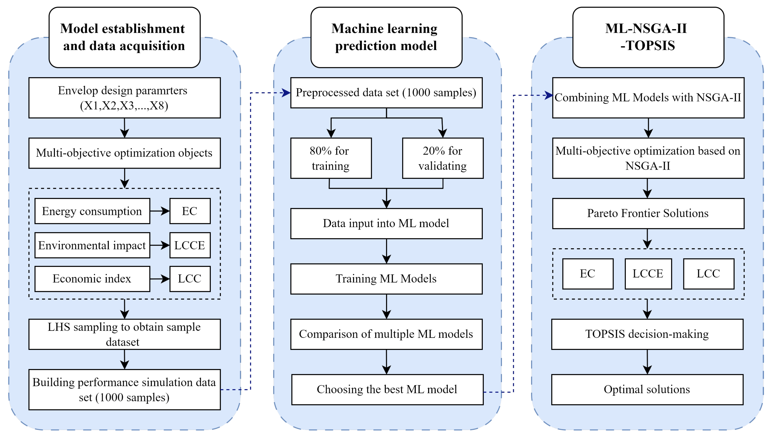
As demonstrated in Figure 1, the proposed residential building energy-saving renovation optimization framework consists primarily of the following six stages:

(1) Develop a building energy simulation model for the reference building.

(2) Identify the building envelope design variables and the optimization objectives.

(3) Conduct a sensitivity analysis on the building renovation design variables to determine the impact trends on the optimization objectives.

(4) Apply the Latin Hypercube Sampling (LHS) algorithm to generate a representative database of simulation cases, which is then used to validate the reliability of the ML models.

(5) Integrate ML models with NSGA-II to obtain the Pareto solution set.

(6) Use the entropy-weighted multi-criteria method to determine the weights assigned to different optimization objectives and identify the appropriate retrofit strategy based on stakeholder preferences.

2.1. Design Variables for Optimization

In the field of building renovation, measures oriented toward enhancing energy efficiency in buildings can directly contribute to the mitigation of greenhouse gas emissions and thus merit the highest possible priority [45,46]. Previous studies outlined the potential of residential building envelope renovation for energy savings, pointing out that envelope renovation can substantially enhance the energy efficiency of residential buildings, which is why this area is given higher priority for renovation [22,23,47,48]. Therefore, in order to reduce the solution space and the model’s complexity, this study selects passive energy-saving design strategies explicitly focused on the renovation of building envelopes as decision variables, including airtightness, depth of the south overhang shading system, type of windows, and insulation type and thickness of the walls and roof [49]. For the above decision variables, the depth of the south overhang shading system and the insulation thickness for the walls and roof are continuous variables. In contrast, the window types, airtightness, and insulation type of the walls and roof are regarded as discrete variables.

The outcomes of any optimization process depend heavily on the bounds and probability distribution of the optimized variables. This study conducted a quantitative evaluation to assess the relative importance of the various components of energy, cost, and ${\mathrm{CO}}_2$ emissions. The thermal characteristics of the building envelope elements are fully described based on the national and local building codes for conventional design and energy efficiency design [50,51]. This study obtained the financial implications of the components through market research and supplier quotations.

Table 1. Design variables of building retrofit strategies.

Design Variables		Range and Interval	Price	CEF
			[$/m3]	$\mathbf{[}{\mathbf{kgCO}}_{\mathbf{2}}\mathbf{e}\mathbf{/}\mathbf{t}\mathbf{]}$
Insulation type	EPS	0.041 $\mathrm{W}/{\mathrm{m}}^2·\mathrm{K}$	49.6	5020
	XPS	0.033 $\mathrm{W}/{\mathrm{m}}^2·\mathrm{K}$	93.7	5020
	Rock wool	0.045 $\mathrm{W}/{\mathrm{m}}^2·\mathrm{K}$	74.4	1980
Insulation thickness	South wall	100∼300; 20 [mm]	-	-
	North wall	100∼300; 20 [mm]	-	-
	East/West wall	100∼300; 20 [mm]	-	-
	Roof	200∼300; 20 [mm]	-	-
Shading	South overhang	0∼1500; 100 [mm]	27.5	28,500

and

Table 2. Glazing types for retrofit.

No.	Glazing Type	U-Value	SHGC	Cost	CEF
		$\mathbf{[}\mathbf{W}\mathbf{/}{\mathbf{m}}^{\mathbf{2}}\mathbf{·}\mathbf{K}\mathbf{]}$		[$/m3]	$\mathbf{[}{\mathbf{kgCO}}_{\mathbf{2}}\mathbf{e}\mathbf{/}\mathbf{t}\mathbf{]}$
W1	Double-glazed glass	2.59	0.75	106.8	121
W2	Double-glazed high-transmission heat-reflective glass	2.58	0.61	122.7	121
W3	Double-glazed low-transmission heat-reflective glass	2.44	0.35	122.7	121
W4	Double-glazed glass (Low-E)	1.79	0.43	126.8	121
W5	Double-glazed glass (argon)	1.44	0.45	165.4	121
W6	Triple-glazed low-transmission glass (Low-E)	1.35	0.27	261.9	194
W7	Triple-glazed high-transmission glass (Low-E)	1.23	0.42	317.0	194
W8	Triple-glazed high-transmission glass (Low-E, argon)	1.01	0.27	358.3	194

provide a comprehensive overview of the potential decision variables and their associated ranges of variability and constraints, including material costs and carbon emission factors (CEFs). The balanced optimization model estimates the configuration of the building based on optimization objectives using eight design variables. A comprehensive evaluation yielded 4.32 × ${10}^7$ combinatorial designs.

2.2. Optimization Objectives

In energy renovation of residential buildings, improving energy performance, reducing environmental impact, and ensuring an acceptable initial investment and payback period under realistic constraints are most important. The following three objective functions are thus addressed for the multi-criteria decision-making model in this paper: energy consumption (EC), life-cycle carbon emissions (LCCE), and life-cycle cost (LCC).

2.2.1. Energy Consumption

In this study, the total energy consumption is mainly composed of annual heating and cooling energy consumption. The mechanical ventilation rate was standardized at one air change per hour across all simulation cases, with supply air temperatures set to 20 °C for heating during winter and 26 °C for cooling during summer. The hourly simulations were conducted throughout the year, with a frequency of six times per hour. This calculation excludes fluctuations in the energy consumption of electronic equipment and domestic hot water, which do not vary significantly during the building’s operation time. The air-conditioning system is regarded as the optimal unit for heating and cooling, with coefficients of performance (COP) of 0.92 and 3, respectively. The energy consumption calculation formula is as follows:

$$EC={\displaystyle \frac{Q_H}{CO{P}_H}}+{\displaystyle \frac{Q_C}{CO{P}_C}}+E_L$$

(1)

where $\mathrm{EC}$ is the energy consumption; ${\mathrm{Q}}_{\mathrm{C}}$ denotes the cooling energy demand; ${\mathrm{Q}}_{\mathrm{H}}$ represents the heating energy demand; ${\mathrm{E}}_{\mathrm{L}}$ denotes the lighting energy consumption; ${\mathrm{COP}}_{\mathrm{C}}$ is the efficiency of the cooling system; and ${\mathrm{COP}}_{\mathrm{H}}$ is the efficiency of the heating system.

2.2.2. Life-Cycle Cost

This study employed the life-cycle cost as the index for evaluating economic indicators, encompassing the present values of both the initial investment and the costs incurred throughout the building’s operational lifespan. In order to evaluate the economic feasibility of a building renovation project, it is essential to consider the initial investment and the life-cycle energy savings achieved once the program is implemented. Given that typical existing residential buildings constructed in severe cold climate regions in China during the 1980s have a typical lifespan of 70 years, it is crucial to consider the remaining operational lifespan when planning a renovation project; a renovated building typically has a lifespan of 20 to 40 years. Consequently, this study uses a 30-year life cycle and employs the net present value method to calculate life-cycle costs, incorporating the time value of money. The calculation formula is as follows:

$$LCC=C_{inv,j}+\sum _{i=1}^n{\displaystyle \frac{C_{m,j}}{{(1+r)}^i}}+\sum _{i=0}^{n}a(r_e,i)·C_{a,j}$$

(2)

$$C_{m,j}=8\%·C_{inv,j}$$

(3)

$$C_{a,j}={\displaystyle \frac{Q_H}{CO{P}_H}}·{\mu }_{coal}·P_{coal}+E_C·P_{elec}$$

(4)

where ${\mathrm{C}}_{\mathrm{inv},\mathrm{j}}$ is the investment cost for the building retrofitting strategy; ${\mathrm{C}}_{\mathrm{m},\mathrm{j}}$ denotes the cost of maintenance in the i-th year following the renovation; the annual maintenance cost is hypothesized to be 8% of the initial investment; ${\mathrm{C}}_{\mathrm{a},\mathrm{j}}$ is the annual cost for energy; ${\mu }_{\mathrm{C}}$ is the heating energy to coal conversion factor, with a value of 0.36 in this study; ${\mathrm{P}}_{\mathrm{coal}}$ is the local coal price; ${\mathrm{P}}_{\mathrm{elec}}$ is the local electricity price; and $\mathrm{a}$ represents the present value factor.

The net present value (NPV) method was employed to calculate the life-cycle costs, incorporating the time value of money, inflation, and energy price escalation. The following formula was used:

$$a={\displaystyle \frac{1-{(1+r_e)}^{-i}}{r_e}}$$

(5)

$$r_e={\displaystyle \frac{r-e}{1+e}}$$

(6)

$$r={\displaystyle \frac{r_i-f}{1+f}}$$

(7)

where $\mathrm{n}$ is the number of years for the operation, assumed to be 30 in this study; $\mathrm{i}$ is the number of years that have elapsed since the original year; ${\mathrm{r}}_{\mathrm{e}}$ is the rate modified to account for market energy price escalation; $\mathrm{r}$ is the effective interest rate; ${\mathrm{r}}_{\mathrm{i}}$ is the interest rate, assumed to be 0.07 in this study; $\mathrm{f}$ is the inflation rate, assumed to be 0.02; and $\mathrm{e}$ is the cost of total energy escalation during the study period above the rate of inflation, assumed to be 0.012 in this study.

These parameters were chosen to align with typical market trends in the region, aiming to capture both short-term and long-term economic impacts. While this study does not explicitly model material cost volatility, future research could incorporate sensitivity analyses to better understand the impact of fluctuating material prices on life-cycle costs.

2.2.3. Life-Cycle Carbon Emission

The term ‘life-cycle carbon emission’ refers to the total amount of carbon emissions, including the embodied carbon emissions generated during the manufacturing and shipping of retrofit materials, as well as those from total building energy consumption during operational phases, serving as a comprehensive measure of environmental impact. A carbon emission factor (CEF), derived from the national building carbon calculation standard, was used to quantify both the embodied carbon emissions and energy-related emissions of building materials [52]. The objective function is described as follows:

$$LCCE=\sum _{j=1}^J{N}_j·f_j+n·\left[E_H·{\mu }_{coal}·f_{coal}+(E_C+E_L)·f_{elec}\right]$$

(8)

where $\mathrm{j}$ denotes the material type for renovation; ${\mathrm{N}}_{\mathrm{j}}$ represents the specific material quantity; ${\mathrm{f}}_{\mathrm{j}}$ is the CEF for the particular material; ${\mathrm{f}}_{\mathrm{coal}}$ denotes the CEF for coal, which is 2.27 in this study; and ${\mathrm{f}}_{\mathrm{elec}}$ represents the CEF for electricity, which is 1.15 in this study.

2.3. Sensitivity Analysis

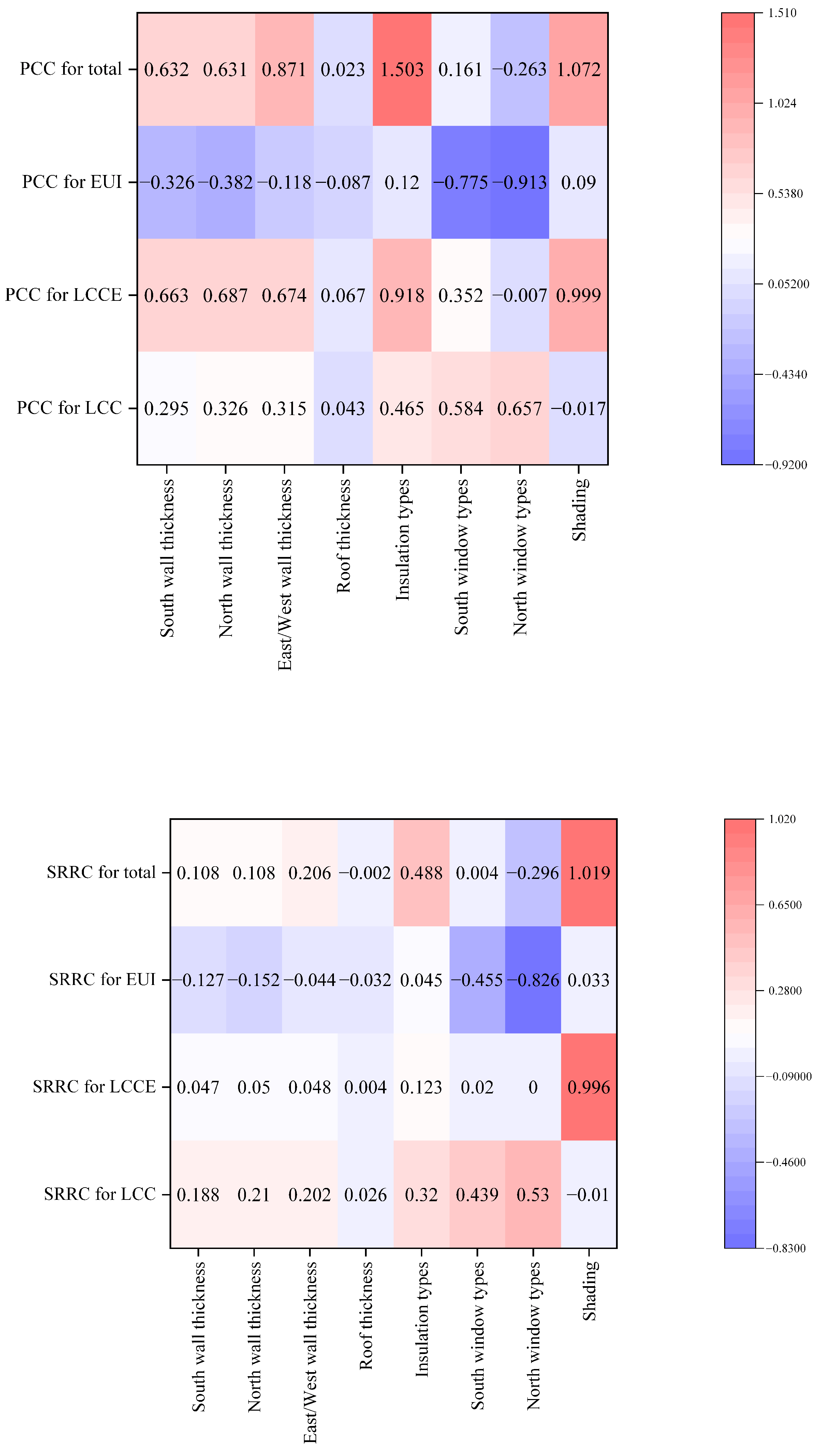
Sensitivity analysis (SA) has been widely utilized in building performance simulations to determine the pivotal factors that substantially impact optimization objectives, as evidenced by numerous studies [53,54]. Regression techniques are favored among the various global SA methods due to their ease of implementation and relatively moderate sample size requirements [53]. Notably, the standardized rank regression coefficient (SRRC) and partial correlation coefficient (PCC) stand out for their effectiveness in dealing with correlated input variables. These two indices can efficiently isolate the effects of variable correlations, thereby enabling a more precise evaluation of the influence of each variable on the target outcome [55]. Therefore, this study uses SRRC and PCC methods to investigate the influence of building renovation strategies on specified objectives and to uncover the underlying correlations between these strategies and optimization objectives.

2.4. Machine Learning Modeling

For machine learning (ML) training, a larger dataset is needed to enhance the training process and improve model accuracy. Previous studies have demonstrated the benefits of utilizing more extensive datasets [56]. To address this limitation, this study uses the Latin Hypercube Sampling (LHS) method to generate the sample space [57]. LHS is a stratified sampling method commonly applied in Monte Carlo simulations and is recognized as a powerful technique for producing small yet statistically representative samples. Compared to random sampling, LHS achieves the same level of statistical accuracy with a smaller sample size [58]. It has been extensively used to establish simulation case databases for validating machine learning models, particularly in residential building energy optimization [59] and building energy retrofitting [10,60].

For building optimization, the sample size required for LHS is typically ten times the number of design variables, influenced by the complexity of the interactions between these variables [46]. This size is considered sufficient if the probability density function stabilizes toward uniformity, effectively representing the entire building library. This study determined a sample size of 1000 cases based on the number of design variables and their interactions. The LHS method generated a matrix that effectively represents diverse building configurations. These configurations were then simulated to populate the database used in the machine learning model. To train and validate the machine learning model, the dataset was split into two subsets: 80% of the sample was used for training, and 20% was reserved for validation. The training step involved optimizing the model’s weighting biases to improve predictive accuracy, while validation ensured the robustness and reliability of the model’s predictions.

To ensure a comprehensive analysis, four different ML models were compared: fast random forest (FRF), light gradient boosting machine (LightGBM), multivariate linear regression (MVLR), and artificial neural network (ANN). These models were selected due to their widespread use in predictive modeling and optimization tasks, as well as their potential to perform well in energy performance prediction for building retrofits. The performance of each model was evaluated using four statistical indicators: the coefficient of determination (R²), root mean square error (RMSE), mean square error (MSE), and mean absolute error (MAE). These metrics provide insights into the accuracy of predictions from different perspectives.

R² measures the proportion of variance in the dependent variable explained by the model. Higher values indicate better model performance.

RMSE quantifies the standard deviation of residuals, representing the average distance between the predicted and actual values. Smaller values indicate better predictions.

MSE calculates the average of squared differences between the predicted and actual values, with smaller values reflecting better accuracy.

MAE assesses the average magnitude of prediction errors, with lower values indicating smaller prediction errors.

By combining these indicators, the study ensures a rigorous evaluation of each model’s accuracy, efficiency, and overall performance. The formulas for calculating these metrics are as follows:

$$R^2=1-{\displaystyle \frac{{\sum }_{i=1}^n{(y_i-{\widehat{y}}_i)}^2}{{\sum }_{i=1}^n{(y_i-\overline{y})}^2}}$$

(9)

$$RMSE=\sqrt{{\displaystyle \frac{{\sum }_{i=1}^n{(y_i-{\widehat{y}}_i)}^2}{n}}}$$

(10)

$$MSE={\displaystyle \frac{{\sum }_{i=1}^n{(y_i-{\widehat{y}}_i)}^2}{n}}$$

(11)

$$MAE={\displaystyle \frac{{\sum }_{i=1}^n|y_i-{\widehat{y}}_i|}{n}}$$

(12)

where $\mathrm{n}$ denotes the number of samples, $\mathrm{i}$ represents the number of case studies in the cluster, ${\mathrm{y}}_{\mathrm{i}}$ denotes the actual value of a sample, ${\widehat{\mathrm{y}}}_{\mathrm{i}}$ represents the predicted value of a sample, and $\overline{\mathrm{y}}$ represents the mean of the actual values.

2.5. Multi-Criteria Decision Method

The evolutionary generation algorithm is a fundamental tool for addressing multi-criteria decision-making problems; it generates a set of non-dominated solutions and facilitates subsequent preference-based decision making [61,62]. It is evident that, within the scope of these methodologies, NSGA-II is particularly well suited for resolving optimization problems encompassing three or more objectives. Consequently, it is extensively employed for multi-criteria decision-making processes in the context of building energy renovation [63]. Additionally, TOPSIS has been widely used for multi-objective decision making in building energy-saving renovation projects [64,65,66]. TOPSIS evaluates the closeness of different solutions to an ideal target. Thus, the entropy-weighted TOPSIS ranking model with the Mahalanobis distance method was used in this study [67]. For building renovation decision making, where energy performance, economic considerations, and sustainability are equally important, the weights for the three optimization objectives were set to be equal.

The following equations show the calculation of the decision matrix, the Mahalanobis distance, and the relative closeness.

(1)

Normalize the Decision Matrix

The normalized decision matrix element $r_{ij}$ is calculated as

$$r_{ij}={\displaystyle \frac{x_{ij}}{\sqrt{{\sum }_{i=1}^m{x}_{ij}^2}}}$$

(13)

(2)

Calculate the Mahalanobis Distance

a. 

The Mahalanobis distance from solution $S_i$ to the ideal solution $A^{+}$ is given by

$$D_i^{+}=\sqrt{{(v_i-A^{+})}^T{C}^{-1}(v_i-A^{+})}$$

(14)

b. 

The Mahalanobis distance from solution $S_i$ to the negative ideal solution $A^{-}$ is given by

$$D_i^{-}=\sqrt{(v_i-A^{-}{)}^T{C}^{-1}(v_i-A^{-})}$$

(15)

(3)

Compute the Relative Closeness

The relative closeness $C_i$ for each solution is calculated as

$$C_i={\displaystyle \frac{D_i^{-}}{D_i^{+}+D_i^{-}}}$$

(16)

Each solution is ranked by its value of $C_i$, with higher values indicating a better solution for $S_i$, and lower values indicating a less desirable solution.

3. Case Study

3.1. Reference Building

The present study constructed a reference model for typical existing residential buildings in Shenyang, China, which has a severely cold climate. The reference building represents a typical residential structure built in the region during the 1980s (Figure 2). It is a typical seven-floor construction with a 3519 ${\mathrm{m}}^2$ total floor area and 63 apartments, each with a ceiling height of 2.7 m (Figure 3). A comprehensive investigation and collation of information on the envelope structures of existing residential buildings were conducted. The investigation indicated that a significant number of local residential buildings constructed in the 1980s were not equipped with insulation layers. Two layers of single-pane glass were used for the windows without broken bridge frames. Since 2022, the government has carried out large-scale renovations of existing residential buildings according to local residential building energy-saving design standards [51]. The renovation added 100 mm EPS to the exterior wall and 200 mm to the roof. The windows remained unchanged, consisting of two layers of single-pane glass.

Table 3. Building envelope and material properties.

Construction Component	Layers (from Exterior to Interior)	Thickness	Conductivity	Density	Specific Heat
		[mm]	[W/m·K]	$\mathbf{[}\mathbf{kg}\mathbf{/}{\mathbf{m}}^{\mathbf{3}}\mathbf{]}$	[J/kg·K]
Roof	Cement mortar surface layer	20	0.93	1800	1050
	EPS insulation	200	0.041	20	1380
	Reinforced concrete slab	100	1.74	2500	920
	Cement mortar surface layer	20	0.93	1800	1050
Exterior wall	Cement mortar surface layer	20	0.93	1800	1050
	EPS insulation	100	0.041	20	1380
	Brick	370	0.81	180	1050
	Cement mortar surface layer	20	0.93	1800	1050
Exterior window	Single-glazed plastic window	6	0.99	2528	880

presents the calculated heat transfer coefficients of the exterior walls, roofs, floors, and exterior windows, as well as the thermal performance parameters of the residential building envelope in this case.

Table 4. Internal heat-gain schedule.

Internal Heat Gain		Weekday	Weekend
Occupant	100 W/occupant	0:00–8:00 and 18:00–24:00	0:00–24:00
Artificial lighting	10 $\mathrm{W}/{\mathrm{m}}^2$	-	-
Refrigerator	120 W	Always on	-
Television	55 W	19:00–22:00	10:00–16:00 and 19:00–22:00

presents the internal heat gain from artificial lighting, equipment, and three occupants per unit, along with the typical workday schedule for each residential unit. Despite the absence of shading overhangs in the reference building, their potential inclusion was explored in the subsequent parametric simulations. Specifically, overhangs above south-facing windows were modeled, with their depth being a key design parameter under optimization. Conversely, no external shading devices were considered for north- and east-facing windows.

3.2. Monitoring and Calibration

Since measuring the actual airtightness of the case study building was not feasible, we referred to former studies on the airtightness of residential buildings [68,69], a parametric analysis was conducted using a building model with varying airtightness values, ranging from 0.0001 to 0.0009 ${\mathrm{m}}^3/\mathrm{s}\mathrm{per}{\mathrm{m}}^2@4\mathrm{Pa}$. The impact of these different scenarios on the building’s performance was assessed, and the model’s accuracy was validated by comparing the simulated results with the measured indoor temperatures on-site, allowing us to estimate the building’s actual airtightness. Hourly indoor temperature data were recorded using the Testo 174H temperature testing instrument between 18 April and 26 April 2024 under free-running conditions. The data were collected in a south-facing bedroom, with measurement points situated 1 m from the windows and readings taken at 15 min intervals. NMBE and cv(RMSE) were used to quantify the error between the measurement and simulation data. This study followed the ASHRAE Guideline 14-2002 [70], a standard method for calibrating building models that provides acceptable calibration accuracy limits. For hourly data, the acceptable limits are $-10\%\le {\mathrm{NMBE}}_{\mathrm{hourly}}\le 10\%$ and ${\mathrm{cv}\left(\mathrm{RMSE}\right)}_{\mathrm{hourly}}\le 30\%$, while for monthly data, the limits are $-5\%\le {\mathrm{NMBE}}_{\mathrm{monthly}}\le 5\%$ and ${\mathrm{cv}\left(\mathrm{RMSE}\right)}_{\mathrm{monthly}}\le 15\%$. NMBE and cv(RMSE) were calculated using the following equations:

$$\mathrm{NMBE}={\displaystyle \frac{{\sum }_{i=1}^n\left(y_i-{\widehat{y}}_i\right)}{{\sum }_{i=1}^n{y}_i}}$$

(17)

$$\mathrm{cv}\left(\mathrm{RMSE}\right)={\displaystyle \frac{\sqrt{\frac{1}{n}{\sum }_{i=1}^n{\left(y_i-{\widehat{y}}_i\right)}^2}}{\overline{P}}}$$

(18)

where $y_i$ denotes the measured data; ${\widehat{y}}_i$ is the predicted value; i indicates the number of case studies in the cluster; n is the number of samples; and $\overline{P}$ represents the average of the actual values of the sample.

As shown in

Table 5. Calibration for the airtightness of the case study.

Hypothetical Airtightness	0.0001	0.0002	0.0003	0.0004	0.0005	0.0006	0.0007	0.0008	0.0009
NMBE	−32.09%	−21.44%	−13.44%	−7.22%	−2.24%	1.85%	5.27%	8.16%	10.64%
cv(RMSE)	32.25%	21.73%	13.97%	8.28%	4.82%	4.87%	7.08%	9.55%	11.83%

and Figure 4, when the value of airtightness is 0.0006, the NMBE and cv(RMSE) of the measurement points are 1.85% and 4.87%, respectively, which are within ASHRAE’s error tolerance. Therefore, it can be concluded that the model is well calibrated.

4. Results and Discussion

4.1. Sensitivity Analysis of Design Variables

Figure 5 shows the sensitivity coefficients of the three target objectives for each variable. The results provided by the PCC and SRRC methods consistently assessed the positive and negative impacts of the sensitivity coefficients on the target objectives for the reference building. As expected and consistent with experience, the impacts of the design variables on the three objective functions differed. Increasing the thickness of external insulation and improving the external window glass material were negatively correlated with energy consumption but positively associated with life-cycle costs and carbon emissions. The external windows represented a much higher sensitivity to energy consumption and cost than the external insulation thickness and a lower sensitivity to carbon emissions. While external shading, such as overhangs, has been increasingly applied to address cooling energy demand, particularly in the context of climate change, their carbon emissions during production often outweighed their limited energy-saving potential. This trade-off underscores the importance of carefully evaluating shading design choices in building retrofitting projects, especially in severe cold climates where shading may play a less critical role in the overall energy performance.

The sensitivity analysis results also indicate that the insulation thickness of the south and north walls had a significantly greater impact on energy performance than that of the east and west walls in the reference building, primarily because the latter orientations have comparatively smaller surface areas. Additionally, the roof insulation thickness was found to have the least impact in this case. This finding suggests that optimization strategies can prioritize insulation improvements for the larger orientations, such as the south and north walls in this case study, while simplifying considerations for the east and west walls. Additionally, using different external insulation materials had little impact on energy consumption but a significant impact on carbon emissions and costs, warranting careful analysis when applied.

4.2. Machine Learning Model Performance

This section analyzes the performance of four distinct machine learning algorithms in predicting building energy consumption (EC) based on the given dataset. These machine learning algorithms, which have demonstrated exceptional capabilities in energy prediction tasks in previous studies [10,39,42], included fast random forest, LightGBM, MVLR, and ANN. To evaluate the predictive performance of each model, metrics were employed, including the coefficient of determination (${\mathrm{R}}^2$), mean absolute error (MAE), mean squared error (MSE), and root mean squared error (cv(RMSE)). A model with MAE, cv(RMSE), and MSE values closer to zero, and an ${\mathrm{R}}^2$ value closer to one, is considered to have superior predictive accuracy. The target feature in this analysis was energy consumption (EC), and the performance of each algorithm was assessed to identify the most reliable and efficient approach for energy prediction. The results of this evaluation provide valuable insights into the comparative strengths and weaknesses of these machine learning models.

Figure 6 illustrates box plots of the performance metrics for the four machine learning models used in energy consumption prediction. The results reveal that the LightGBM model outperformed the other three ML models by demonstrating superior performance across all evaluated metrics. Additionally, the ANN and FRF models exhibited nearly identical predictive performance; however, the FRF box plot indicates a greater number of outliers, suggesting that the FRF algorithm generated a higher proportion of poorly performing predictive models. In contrast, the ANN algorithm displayed fewer outliers, indicating more consistent and stable predictive accuracy compared to the FRF model. Among the four models, MVLR exhibited the poorest performance, highlighting its limited capability to address the complexities of energy consumption prediction tasks.

Table 6. Performance comparison of ML models.

Model	MAE	MSE	RMSE	R2
FRF	1.32	2.67	1.63	0.86
LightGBM	0.39	0.29	0.54	0.98
ANN	1.24	2.33	1.53	0.88
MVLR	1.41	2.87	1.69	0.85

provides a detailed comparison of the performance metrics for each machine learning model. The LightGBM model achieves significantly lower MAE, MSE, and RMSE values compared to the other three models, indicating its exceptional predictive performance. In contrast, the higher MAE, MSE, and RMSE values observed for the MVLR, FRF, and ANN models suggest relatively lower prediction accuracy. These findings underscore the suitability of gradient boosting models, such as LightGBM, for handling the inherent complexities of building energy consumption prediction tasks. Their superior accuracy and reliability position them as a more effective solution compared to simpler models. Based on this comparative analysis, the LightGBM model was identified as the optimal choice for predicting building energy consumption due to its outstanding stability and accuracy.

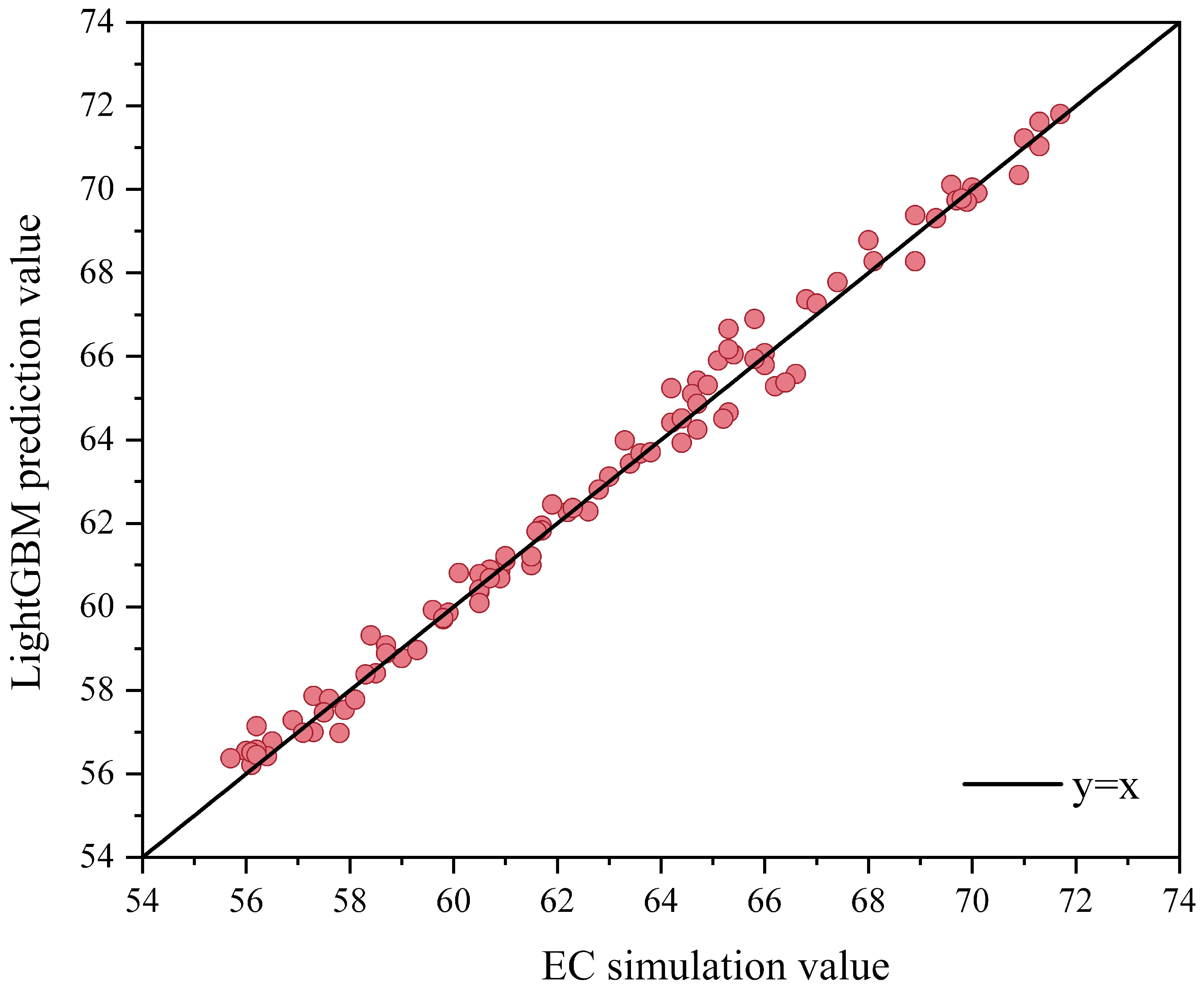
Figure 7 illustrates the regression performance of the LightGBM model in predicting energy consumption (EC). The scatterplot compares the tested EC values (x-axis) with the predicted EC values (y-axis) generated by the LightGBM model. The results demonstrate a strong linear relationship between the predicted and true values. This indicates that the LightGBM model achieves high predictive accuracy and effectively captures the relationship between the input features and energy consumption. The clustering of points along the diagonal further supports the model’s stability and reliability in predicting energy consumption across the dataset.

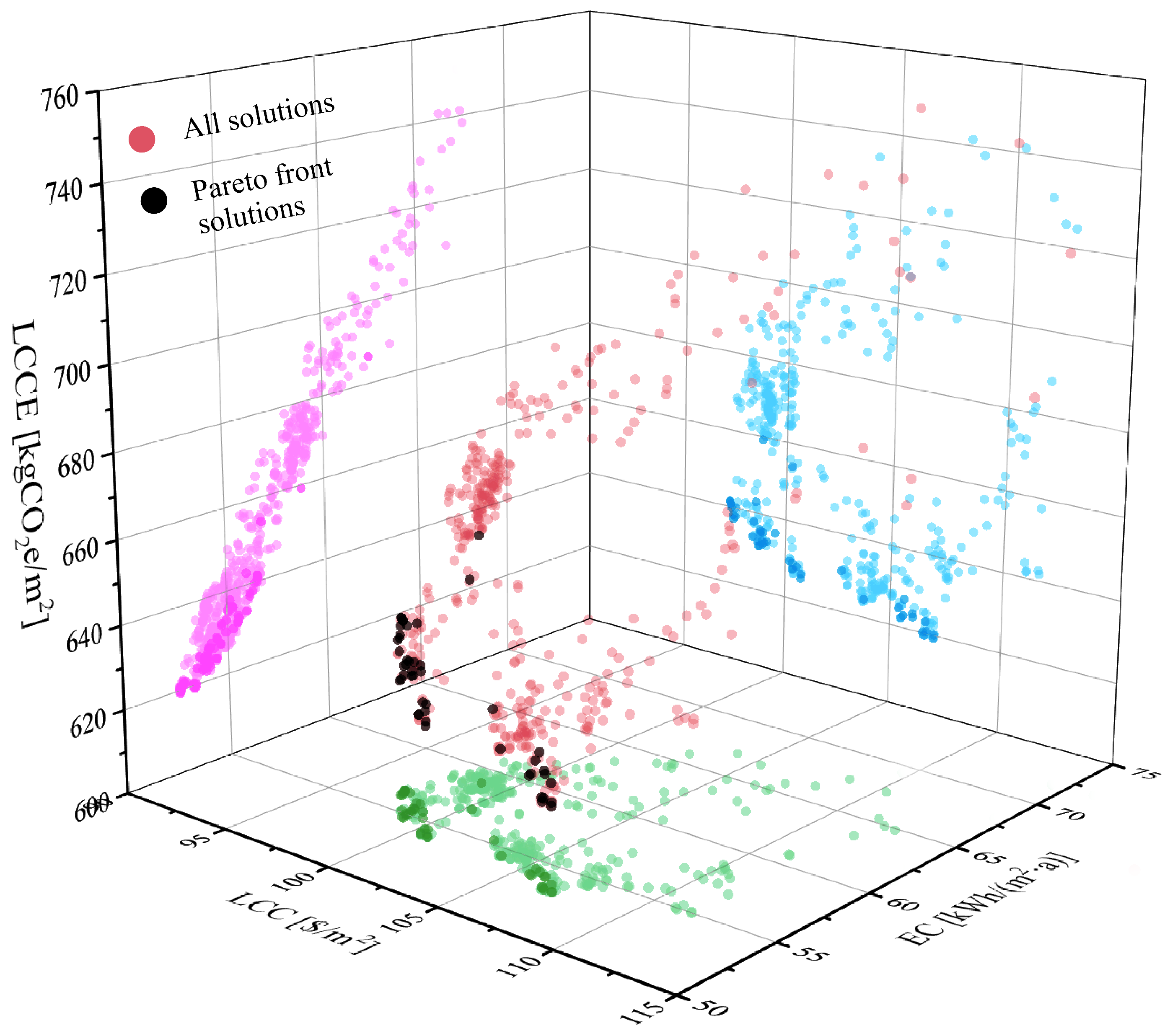
4.3. The Optimal Pareto Front Solution Sets

The optimization procedure used to create the model and the run results are described below. Eight design variables and 1.44 × 10⁷ combinatorial designs were evaluated in the case study. After 63 generations, the Pareto solutions successfully converged in less than 3 min. This study used the Intel Core i9-13950HX processor for training. The machine learning surrogate model significantly shortened the required time, making the optimization process a viable approach in the context of engineering practice.

Figure 8 shows the optimization results and Pareto front solutions, illustrating the Pareto front for minimizing energy consumption, carbon emissions, and life-cycle costs. Each solution represents an optimized building envelope design that balances the three objectives. As anticipated, trade-offs are evident between the objectives. The dispersion of solutions is influenced by the case study’s characteristics and the notable differences in the market prices and embodied carbon emissions of building envelope materials.

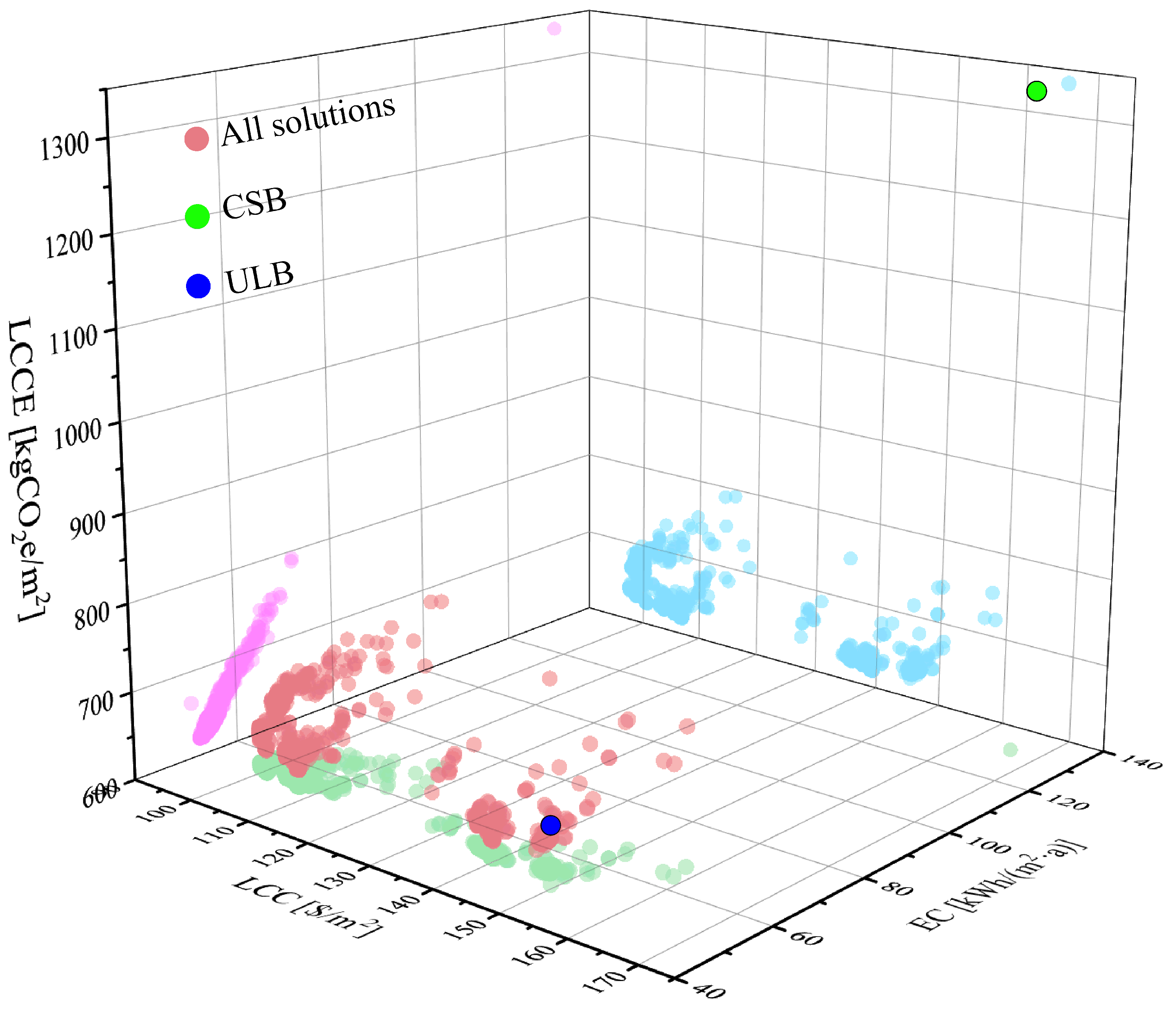
As shown in

Table 7. Comparison of single-objective solutions with the case study building and ultra-low-energy building.

Design Solutions		CSB	ULB	Minimal EC	Minimal LCCE	Minimal LCC
Insulation type		EPS	XPS	XPS	EPS	EPS
Thickness [mm]	${\mathrm{Wall}}_N$	100	300	300	220	300
	${\mathrm{Wall}}_S$	100	300	300	160	300
	${\mathrm{Wall}}_{E/W}$	100	300	260	280	260
	Roof	200	300	240	220	300
Glazing type	${\mathrm{Win}}_N$	Single-plane	W8	W8	W8	W8
	${\mathrm{Win}}_S$	Single-plane	W8	W7	W4	W7
Shading [mm]		0	1500	0	0	0
EC [kWh/${\mathrm{m}}^2·\mathrm{a}$]		131.60	51.20	52.59	52.63	56.53
LCCE [${\mathrm{kgCO}}_2\mathrm{e}/{\mathrm{m}}^2$]		1335.24	663.59	620.24	619.32	641.40
LCC [$/${\mathrm{m}}^2$]		165.85	149.25	139.07	139.39	97.24

, a comparative analysis was performed on the design solutions pertaining to the different energy efficiency standards, namely the case study building (CSB) and ultra-low-energy building (ULB), with the solutions corresponding to the three minimal objectives derived from the Pareto solutions. The CSB model represents the original design retrofitted based on the local energy efficiency design standard [51], and the ULB model is derived from the latest local energy efficiency design standard for ultra-low-energy residential buildings [71]. The values of all the design variables for the renovation strategies, as well as the corresponding EC, LCCE, and LCC values, are listed.

Table 8. Comparison between minimal single-objective optimization results, case study building, and ultra-low-energy building.

Design Solutions		Minimal EC	Minimal LCCE	Minimal LCC
Compared with CSB	EC	−60.04%	−60.01%	−57.04%
	LCCE	−53.55%	−53.62%	−51.96%
	LCC	−16.15%	−15.96%	−41.36%
Compared with ULB	EC	2.71%	2.79%	10.41%
	LCCE	−6.53%	−6.67%	−3.34%
	LCC	−6.82%	−6.61%	−34.84%

presents a comparison between the minimal single-objective optimization results, case study building, and ultra-low-energy building. Compared with the CSB model, the minimum energy consumption, life-cycle carbon emission, and cost schemes all achieved significant reductions. The three indicators were reduced to varying degrees, reflecting considerable energy savings, emission reductions, and cost advantages. Compared with the ULB model, the minimum energy consumption scheme in the Pareto solution also reduced energy consumption, carbon emissions, and life-cycle costs to varying degrees. The minimum carbon emission and life-cycle cost schemes significantly reduced carbon emissions and life-cycle costs by decreasing the use of building envelope materials, thereby achieving win-win economic and environmental benefits.

Table 9. The ranking of optimal solutions and relative closeness values.

Relative Closeness	A	B	C	D	E
$D_i^{+}$	2.6837	6.6658	8.3124	8.3525	8.6695
$D_i^{-}$	10.4990	6.0726	6.7315	5.8794	5.8662
$C_i$	0.7964	0.4767	0.4475	0.4131	0.4036

presents the top five solutions derived using the entropy-weighted TOPSIS method, evaluated against the criteria of minimizing EUI, LCCE, and LCC. With equal weights of 0.33 assigned to each criterion, the analysis identified solutions exhibiting the highest relative closeness values, signifying their proximity to the ideal solution while maintaining substantial separation from the negative ideal solution. The top-ranked solution achieved a relative closeness of 0.7964, followed sequentially by solutions with relative closeness values of 0.4767, 0.4475, 0.4131, and 0.4036. These rankings underscore the balanced integration of all criteria in the evaluation process, demonstrating the method’s ability to prioritize Pareto-optimal solutions effectively. The findings highlight the utility of entropy-weighted TOPSIS as a robust tool for informed decision making in multi-criteria optimization scenarios.

As shown in Figure 9 and

Table 10. Top five multi-objective optimization solutions.

Design Solutions		CSB	ULB	A	B	C	D	E
Insulation type		EPS	XPS	XPS	EPS	EPS	EPS	EPS
Thickness [mm]	${\mathrm{Wall}}_{\mathrm{N}}$	100	300	220	220	300	280	300
	${\mathrm{Wall}}_{\mathrm{S}}$	100	300	160	160	160	160	160
	${\mathrm{Wall}}_{\mathrm{E}/\mathrm{W}}$	100	300	260	260	260	260	260
	Roof	200	300	220	220	220	220	240
	${\mathrm{Win}}_{\mathrm{N}}$	Single-plane	W8	W3	W7	W8	W8	W8
	${\mathrm{Win}}_{\mathrm{S}}$	Single-plane	W8	W5	W4	W8	W7	W7
Shading [mm]		0	1500	0	0	0	0	0
EC [kWh/${\mathrm{m}}^2·\mathrm{a}$]		131.6	51.2	62.42	58.83	54.65	54.91	54.64
LCCE [${\mathrm{kgCO}}_2\mathrm{e}/{\mathrm{m}}^2$]		1335.24	663.59	686.54	659.21	627.73	630.20	627.88
LCC [$/${\mathrm{m}}^2$]		165.85	149.25	114.50	98.83	144.66	134.79	135.16

, in comparison to the CSB model, all selected optimal solutions resulted in average energy savings of 56.62%, reductions in carbon emissions of 51.60%, and 24.27% decreases in life-cycle costs. In comparison to the ULB model, all selected optimal solutions resulted in a significant reduction in carbon emissions and life-cycle costs by 2.60% and 15.85%, respectively, despite slightly higher energy consumption.

The majority of optimal solutions recommended EPS as the primary insulation material for the building envelope, which is attributed to its relatively low incremental cost and acceptable performance.

Across all selected solutions, the insulation thickness on the south-facing wall was reduced to 160 mm, a noticeable decrease compared to the ULB model. This adjustment reflects the lower energy demand for the south-facing wall, given its higher solar exposure and heat-gain potential. Similarly, the east and west walls were recommended to have a reduced insulation thickness of 260 mm, as these orientations have a minimal overall impact on energy performance. In contrast, the north-facing wall was suggested to maintain a 280–300 mm thickness for enhanced thermal performance. However, reducing the north wall insulation to 220 mm could significantly lower life-cycle carbon emissions (LCCE) at the expense of energy efficiency, leading to higher life-cycle costs (LCC). This trade-off arises because, in this case study, energy costs constitute a substantial portion of the total 30-year life-cycle costs.

The optimization also highlights the importance of window selection. Solutions C, D, and E recommended using high-performance windows (W7 or W8) with triple-glazed, high-transmission Low-E glass. These windows help minimize life-cycle costs and carbon emissions while maintaining energy efficiency. Conversely, solution B recommended using lower-cost windows (W4 or W5, double-glazed), which increase annual energy consumption by 14.90% compared to the ULB benchmark. However, over a 30-year life cycle, this approach significantly reduces life-cycle costs (33.78%) and achieves a marginal reduction in life-cycle carbon emissions (0.66%) while also minimizing the initial investment for renovation materials.

In addition, the overhang depth for south-facing shading was inappropriate, aligning with the findings of the sensitivity analysis. The primary advantage of south-facing shading is that it reduces a minor portion of the summer cooling load. However, the overhang depth is excessive, increasing the energy used for lighting and winter heating. Furthermore, this approach may have a detrimental impact on the environment due to the considerable CEF value of the shading material, which does not contribute to reducing carbon emissions.

Overall, the results illustrate a balanced approach, where selecting insulation materials, thickness, and window types can be tailored to meet specific objectives, such as minimizing lifecycle carbon emissions, reducing costs, or maintaining high energy efficiency.

5. Conclusions

The present study provides a valuable illustration of the efficacy of automated machine learning, in conjunction with the NSGA-II algorithm, in the domain of multi-criteria decision making for the energy-saving retrofitting of residential buildings. The research results reveal that the utilization of a surrogate model can lead to a substantial reduction in optimization time, facilitating rapid and effective analysis and prediction of the effects of diverse energy-saving renovation strategies and identifying the optimal balance among total energy demand, life-cycle carbon emissions, and cost targets. Among the four machine learning algorithms evaluated, the light gradient boosting machine algorithm emerged as the most efficient and accurate model for predicting building energy performance.

Through the metaheuristic algorithm and entropy-weighted decision-making mechanism, the obtained Pareto front results, compared to the original design of the case study building, which followed the national energy efficiency design code, showed significant improvements in all three objectives after optimization. The optimal solutions reduced energy consumption by 56.62%, carbon emissions by 51.60%, and life-cycle cost by 24.27%. This highlights the necessity of further retrofitting existing buildings that have already met the national energy efficiency standard from both an energy-saving and life-cycle environmental perspective. Compared to the ultra-low-energy building energy standard, all selected optimal solutions significantly reduced energy emissions by 2.60% and the life-cycle cost by 15.85%.

The present study contributes significantly to building energy conservation in two respects: Firstly, it proposes a novel framework that integrates a machine learning surrogate model with a heuristic optimization algorithm and entropy-weighted decision-making mechanism. This novel framework introduces original methodologies for the multi-criteria evaluation process in energy-saving renovation for existing residential buildings. The novel methods simplify the steps of model selection and hyperparameter adjustment, enhancing the prediction model’s accuracy. Secondly, the optimal solution can assist residents in optimizing building energy use, facilitating the transition to fossil fuel alternatives, and reducing dependency on traditional energy sources. From economic and environmental viewpoints, these optimal solutions are highly suitable for future renovation strategies that promote sustainable and cost-effective building performance improvements.

This study also has limitations that are worth noting. As climate change progresses, long-term building renovation strategies must incorporate projections of future climatic conditions to ensure the durability and efficacy of implemented solutions. Rising temperatures, changing weather patterns, and shifting heating and cooling demands necessitate a climate-responsive approach to retrofitting. For example, in future climate scenarios (e.g., 2050 and 2080), indoor thermal comfort will likely become a critical factor in colder regions, necessitating a re-evaluation of existing retrofit standards and the integration of renewable energy systems, such as photovoltaic panels, to achieve net-zero-energy performance while mitigating carbon emissions. Future studies will focus on conducting urban-scale building energy analyses for residential neighborhoods under projected climate conditions. This broader scope will allow for the development of optimized retrofit strategies at both the individual building and community levels, ensuring that renovation efforts align with the evolving needs of urban areas in response to climate change. Such efforts will enhance energy efficiency and improve urban resilience and adaptability to long-term environmental challenges.