Abstract
Partial discharge (PD) detection plays an important role in online condition monitoring of electrical equipment and power cables. However, the noise of PD measurement will significantly reduce the performance of the detection algorithm. In this paper, we focus on the study of a PD noise reduction algorithm based on improved singular value decomposition (SVD) and multivariate variational mode decomposition (MVMD) for white Gaussian noise (WGN) and periodic narrowband interference signal noise. The specific noise reduction algorithm is divided into three noise reduction processes: The first noise reduction completes the suppression of narrowband interference in the noisy PD signal by the SVD algorithm with the guidance signal. The guidance signal is composed of a sinusoidal signal of the accurately estimated narrowband interference frequency component, and the amplitude is twice the maximum amplitude of the noisy PD signal. The second noise reduction decomposes the noisy PD signal after filtering the narrowband interference signal into k optimal intrinsic mode function by the MVMD after parameter optimization. By calculating the kurtosis value of each intrinsic mode function, it is determined whether it is the PD dominant component or the noise dominant component, and the noise dominant component is subjected to 3σ filtering to obtain the reconstructed PD signal. The third noise reduction uses a new wavelet threshold algorithm to denoise the reconstructed PD signal to obtain the denoised PD signal. The overall noise reduction algorithm proposed in this paper is compared with some existing methods. The results show that this method has a good effect on reducing the noise of PD signals measured in simulation and field.
1. Introduction
Partial discharge (PD) may occur when high voltages are applied across insulators with defects, which has been widely used for online monitoring [1,2]. However, due to the complex and harsh field environment, the PD signal detected online is often accompanied by strong electromagnetic interference [3]. It is difficult to extract pure PD signals. Therefore, it is very important to effectively suppress the noise in the PD signal.
1.1. Relevant Works
The background noise in PD detection mainly includes white noise and periodic narrowband noise [4]. Because the energy of white noise is evenly distributed at all frequencies, the wavelet coefficients of white noise decrease gradually with the increase in the wavelet decomposition scale, so the wavelet transform has a better removal effect on white noise [5,6]. In [7], a wavelet noise reduction method based on ant colony algorithm optimization is proposed. Using continuous derivative threshold function and Ant Colony Optimization (ACO), the global optimum threshold is found, and then the PD signal noise reduction is realized. However, the joint algorithm has obvious shortcomings in time and efficiency. In [8], adaptive dual-tree complex wavelet transform (ADTCWT) is used for PD signal noise reduction. The threshold value of the two-tree complex wavelet is determined by using the adaptive singular value decomposition method, and then the noise reduction is realized. However, the improved system still has oscillation error and will lose the edge of the signal [9]. Paper [9] proposed wavelet threshold and total variation theory for PD signal noise reduction. Through the combination of these two algorithms, the oscillation error can be reduced without the introduction of visible stair error. However, the selection of wavelet base function, wavelet threshold and decomposition level is largely dependent on human experience [10]. Paper [11] directly determines the decomposition layer for noise reduction through the spectral kurtosis diagram of the PD signal, thus avoiding the setting of the threshold coefficient, the parent wavelet and the number of decomposition layers. The results show that this method can remove white noise more effectively. In addition, the modal decomposition method has also received some attention in recent years due to its advantages of no preset basis function and strong adaptability. In [12], a PD signal noise reduction method based on new adaptive ensemble empirical mode decomposition (NAEEMD) is proposed. The noise reduction is accomplished by using a threshold criterion which combines the white Gaussian noise (WGN) spectrum and the mean cycle of energy density. However, the noise reduction method based on EMD or NAEEMD is often unable to eliminate the problem of modal aliasing and endpoint effect. In [13], S_VMD and Sdr_SampEn are used for PD signal noise reduction. The optimal modal parameter k of the VMD algorithm is determined by the Spearman correlation coefficient, and the noise reduction is completed by combining the spatial correlation recursive sample entropy criterion of each intrinsic mode function (IMF) and the wavelet threshold method. However, the Spearman coefficient can only ensure that the noisy PD signal is completely decomposed of the VMD algorithm, and the accurate extraction of PD signal characteristics in the decomposition process is not considered. Paper [14] proposed a noise reduction method to optimize MVMD parameters through image information entropy. Image information entropy is combined with the Pearson correlation coefficient to optimize MVMD modal parameter k to complete noise reduction. It can be seen that when k = 8, the PD signal has the greatest degree of certainty under this decomposition method, and its noise content is relatively small. However, a fixed empirical value is selected for the penalty factor, which is difficult to be universal for the decomposition of noisy PD signals. Moreover, when the content of narrowband interference in the signal is large, the noise reduction effect is not significant.
Narrowband interference signals usually have specific frequency components and high power levels. When the frequency components of narrowband interference are similar to PD signals, EMD, MVMD and other methods may cause modal aliasing, which affects the accurate extraction of PD signals. Therefore, a separate narrowband interference signal filtering method is worth studying. Singular value decomposition (SVD) has a good effect on removing narrowband interference in noisy PD signals [15,16]. After determining the singular value number of narrowband interference by Fourier transform power spectrum, paper [17] effectively eliminates periodic narrowband interference by SVD. Paper [18] proposed to construct a Hankel matrix for SVD of noisy PD signals to realize the separation of narrowband interference subspace and PD signal subspace, so as to complete narrowband interference suppression. However, the reliability of using artificial selection of large singular values to distinguish narrowband interference subspace and PD signal subspace is poor, and it may cause some subspaces of the PD signal to be eliminated. Paper [19] used a K-means clustering algorithm to adaptively distinguish narrowband interference subspace and PD signal subspace. However, the suppression effect on small-amplitude narrowband interference is not further considered. In addition, paper [20] uses the adjustable resolution of the generalized S transform to invert the main frequency part of the PD signal to filter out periodic narrowband noise. However, the selection of adjustment factors α and β is based on experience, and the algorithm has poor adaptability.
1.2. Problems of the Existing Methods
Through the research and analysis of common noise reduction algorithms at home and abroad, some technical difficulties in existing noise reduction methods can be summarized:
(1) When the traditional SVD is used to suppress the narrowband interference, it is difficult to determine the number of singular values of the narrowband interference. If it is not determined properly, it is easy to cause the PD singular value to be eliminated, thus affecting the narrowband interference suppression effect. In addition, when the narrowband interference amplitude is small, the singular value of the narrowband interference may intersect with the PD singular value, and the narrowband interference suppression effect becomes worse.
(2) In the process of iterative decomposition, EMD and EEMD algorithms are prone to modal aliasing and endpoint distortion, which leads to low timeliness of the algorithm and inaccurate feature extraction. If the problem of modal aliasing cannot be eliminated, there will be a large amount of residual noise in the denoised PD signal.
1.3. Contributions
Aiming at some technical difficulties in existing noise reduction methods, this paper proposes improved singular value decomposition (ISVD) and multivariate variational mode decomposition (MVMD) for PD signal noise reduction. Work is performed with respect to the following three aspects:
(1) An adaptive method for accurately determining the amount of narrowband interference is proposed. The total amount of narrowband interference and partial discharge is determined by the good time–frequency aggregation of frequency slice wavelet transform (FSWT) and the small threshold method, and then the amount of narrowband interference is accurately determined by the deviation criterion, which solves the problem that it is difficult to determine the amount of narrowband interference in the method of SVD suppression of narrowband interference.
(2) The improved Rife method is introduced into PD noise reduction research. By shifting the signal frequency to the center region of two adjacent quantization frequencies, the improved Rife method can effectively reduce the estimation error of the narrowband interference signal frequency. The guided signal constructed by this method can effectively suppress the narrowband interference signal in the noisy PD signal even when the narrowband interference amplitude is small.
(3) The marine predator algorithm (MPA) considering minimum average envelope entropy (MAEE) is introduced to optimize the decomposition mode number k and penalty factor α of MVMD. After MPA optimization, the multivariate variational mode decomposition algorithm can decompose the PD characteristic signal with the maximum degree of certainty as the goal, so as to accurately decompose the noisy PD signal.
2. Partial Discharge Signal
2.1. The Simulation Model of PD Signals
A large number of papers and field experiments have proved that PD signals can usually be characterized by four kinds of mathematical models [14,21]. In this paper, three kinds of simulated PD signals are selected: double exponential decay function y1(t), double exponential oscillation decay function y2(t) and single exponential decay function y3(t). The expressions are shown as follows:
where A1, A2 and A3 is the signal amplitude. τ1, τ2 and τ3 are the attenuation coefficients, while fc1 and fc2 are the oscillation center frequency. And the sampling time is 40 μs. The specific parameters of the simulated PD signal are shown in Table 1.

Table 1.
PD simulation parameter settings.
The simulation software used in this paper is MATLAB 2022a. The sampling frequency of the analog signal is 50 MHz. Three types of PD pulse models are introduced, as shown in Figure 1a. y1 appears at N1 = 250, y2 appears at N2 = 650 and y3 appears at N3 = 1325. In order to simulate the noise interference of the PD signal in the actual field, a Gaussian WGN signal with an SNR of −1 dB was superimposed on the pure PD signal shown in Figure 1a.
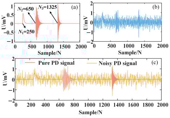
Figure 1.
Simulated PD signal. (a) Pure PD signal; (b) narrowband interference; (c) noisy PD signal.
In addition, there is often a problem of narrowband interference and PD signal aliasing in the actual detection of PD signals. The narrowband interference shown in Figure 1b was superimposed on the pure PD signal, as shown in (4). The specific parameters of narrowband interference are shown in Table 2.
Table 2.
Specific parameter settings.
In (4), Ai, fi and φi represent amplitude, frequency and initial phase angle of narrowband interference.
The PD signal with superimposed noise is shown in Figure 1c, which shows that the pure PD signal has been greatly disturbed by the noise and cannot be extracted.
2.2. Evaluation Criteria for Noise Reduction Effect
In order to evaluate the noise reduction effect of different algorithms, three indexes are introduced for the simulated signal [22] and two indexes are introduced for the field-measured signal [13].
(1) Signal-to-noise ratio (SNR) reflects the ratio of the effective signal to noise. The larger the SNR value, the smaller the residual noise, which is expressed as (5).
(2) Normalized correlation coefficient (NCC) reflects the degree of relatedness of the noise-reduced signal and the pure signal. An NCC value closer to 1 signifies a higher degree of correlation, indicating that the noise-reduced signal closely resembles the pure signal, which is expressed as (6).
(3) Root mean square error (RMSE) reflects the deviation between the denoised signal and the pure signal. The smaller the RMSE value, the smaller the error in amplitude and frequency between the noise-reduced signal and the pure signal, which is expressed as (7).
In (5)–(7), Ssignal is the pure signal, Sdenoised is the denoised signal and N is the number of sampling points.
(4) In the field detection, since the pure PD signal is unknown, the noise reduction effect cannot be judged by SNR, NCC and RMSE. Therefore, in this paper, the Noise Reduction Ratio (NRR) is applied to assess the effectiveness of noise reduction, which is expressed as:
In (8), σ1 and σ2 represent the standard deviations of the field-measured signal and the denoised signal.
(5) ARR evaluates the noise reduction effect from the amplitude of the PD waveform, which is expressed as
In (9), and are the amplitude of the field-measured signal and the noise reduction signal, respectively.
3. Theory Analysis
3.1. FSWT Algorithm
FSWT is a new method of time–frequency analysis proposed by Yan Zhonghong et al. [23]. This method has higher time–frequency resolution and can describe the non-stationary process of the signal delicately, which is suitable for the noise reduction research of PD signals.
The FSWT of a noisy PD signal in the frequency domain can be expressed as
In (10), t is the signal time, is the frequency value, is a constant, is the estimated frequency, * represents a conjugate, is the FFT transform result of the frequency slice function and is the FFT transform result of the noisy PD signal. It can be seen from paper [24] that for the PD signal, has the better time–frequency concentration, so this paper has been selected for its frequency slice function.
Compared with some popular time–frequency analysis methods, STFT limits its time–frequency resolution due to the fixed-window function. The scale of the wavelet basis function of continuous wavelet transform cannot be adjusted according to the frequency distribution of the signal. The center of the time frequency window is not the frequency of the signal, and there is a frequency measurement error [25]. The time–frequency analysis of noisy PD signals is carried out, and the transformation results of several popular time–frequency analysis methods are shown in Figure 2.
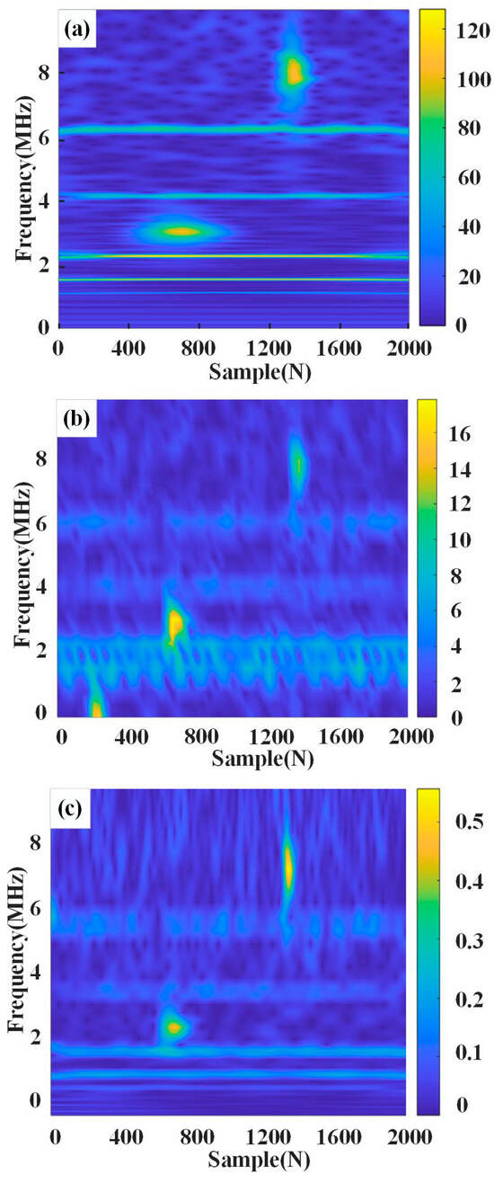
Figure 2.
Comparison of transformation results of different time–frequency analysis methods for noisy PD signals. (a) FSWT; (b) STFT; (c) CWT.
It can be seen from Figure 2 that the time–frequency resolution of the STFT result is poor, and it is difficult to judge the amount of narrowband interference. The time–frequency resolution of the CWT result is slightly better, but the PD signal and the narrowband interference signal are seriously overlapped. The results of FSWT can see clearly the time and frequency characteristics of each signal. The narrowband interference signal has the characteristics of long duration and high intensity, while the frequency distribution of the PD signal is wide and has a time range. These features can be applied to extract the amount of narrowband interference skillfully.
3.2. Skewness Criterion
Skewness is a measure of the direction and degree of skew in data distribution., as shown in (11). The narrowband interference signal obeys the normal distribution, and its skewness value is equal to 0, in theory. However, due to the existence of spectrum leakage, its skewness value is generally less than 0, and the time spectrum distribution has a negative deviation. However, the partial discharge signal obviously deviates from the normal distribution and has a certain time range. The skewness is often greater than 0, and the time spectrum distribution has a positive deviation. Therefore, the skewness value of the time spectrum corresponding to each peak frequency point can be used to distinguish the narrowband interference signal from the partial discharge signal.
3.3. MPA Optimized MVMD
The MVMD algorithm is an extension of the VMD algorithm from one-dimensional to multi-dimensional. By establishing a constrained variational model expression, the consistency of multi-channel data component frequency in the signal decomposition process is guaranteed.
The multi-channel signal is decomposed into k components with the same center frequency and minimized total bandwidth. The corresponding constrained variational optimization problem is expressed as:
In (12), t is time, is the original signal, k is the number of intrinsic modes, is the kth mode of the c channel and is the center frequency of k intrinsic modes.
The Lagrange multiplication operator is introduced to transform (12) from a constrained problem to an unconstrained problem. The associated augmented Lagrange function is illustrated in (13).
The unconstrained problem is solved using the alternating direction multiplier algorithm, with the center frequency update given by (14), completing the adaptive decomposition of multivariate signals.
The modal number k in the MVMD algorithm determines the precision of the decomposition. If the k value is too large, there will be pseudo components in the IMF component. If the k value is too small, it will lead to modal aliasing. The penalty factor α in the MVMD algorithm determines the bandwidth of the IMF component. If the α value is too large, it will affect the fidelity of the reconstructed data. If the α value is too small, it will make some components contain other components. Therefore, the determination of k and α is very important for the decomposition effect of MVMD. In order to solve the above problems, this paper proposes to use the MPA algorithm to optimize MVMD decomposition parameters k and α.
MPA is a meta-heuristic optimization algorithm proposed in 2020 [26], which is derived from the optimal foraging strategy in marine organisms. It searches for the optimal solution by simulating the process of predator preying on prey.
In the MPA framework, the sea represents the global scope of the optimization problem, the elite predator matrix represents the optimum solution in the global range and the prey matrix is the optimum solution obtained in the current iteration. On the basis of the complex interaction of predator and prey, the MPA iteration process is divided into four key links:
(1) Population initialization: the MPA pass (x) randomly determines the initial position in the feasible region and starts the optimization process, as in (15).
In (15), represents the upper bound of the search space, while represents the lower bound. is a random number that falls within the interval [0, 1].
(2) Population optimization iteration consists of three iterative stages: initial, middle and final stages to update the population’s moving step size and position.
(3) The effect of eddy current and artificial fish-gathering device: By simulating the dual effects of ocean eddy current and an artificial fish collection device on the distribution and behavior of marine biological populations in a real marine environment, MPA greatly reduces the probability of a population falling into local optimum by integrating the secondary population renewal mechanism.
(4) Marine memory update: The fitness function value of the prey matrix is calculated, and the elite matrix is updated accordingly. If the convergence requirement is met, the iteration ends, and vice versa.
The specific process of MPA optimizing MVMD parameters is shown in Figure 3:
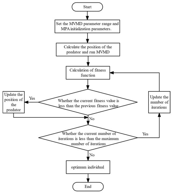
Figure 3.
MPA algorithm optimization of MVMD flow chart.
Envelope entropy is a reflection of the sparseness of a signal. Smaller envelope entropy indicates stronger signal sparsity, higher PD signal certainty and less noise. The average envelope entropy represents the mean of the envelope entropy of all IMF components decomposed by MVMD. The IMFs set with the smallest AEE have the highest degree of determination, which can improve the quality of the noise reduction of the PD signal effectively. Therefore, the MAEE is used as the fitness function to optimize k and α of MVMD, so as to realize the effective decomposition of the PD contaminated signal. The fitness function is defined as follows:
In (16), and are the optimal parameters and is envelope entropy of each modal component , which is calculated by (17) and (18).
In (17) and (18), N is the number of sampling points, is the normalized form of and is the envelope signal of each modal component after Hilbert transform.
In order to verify the effectiveness of AEE as the fitness function, WGN with a step size of 1 dB and from −10 dB to 20 dB is superimposed, respectively, on the pure PD signal in Figure 1a. The input parameter k of MVMD is set to 6, and the α is set to 3000. The value of AEE at each step size is obtained as shown in Figure 4.
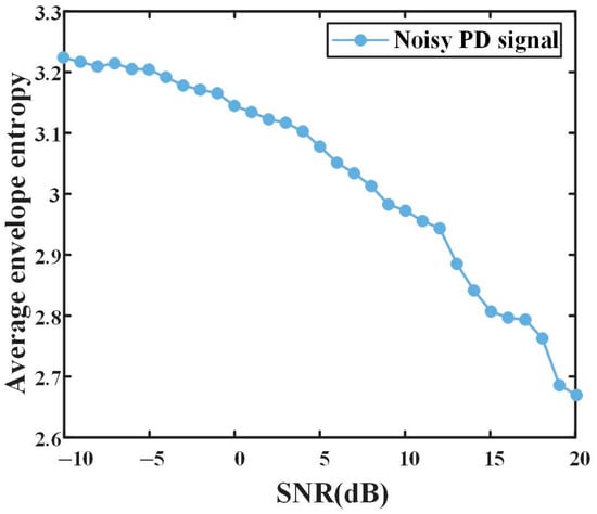
Figure 4.
AEE of different SNRs.
Figure 4 shows AEE decreases as PD signal SNR increases, indicating more certain discharge signals have smaller AEE values.
3.4. Kurtosis Criterion
Kurtosis is a measure of the steepness or sharpness of the data distribution, as shown in (18). Since the WGN and narrowband interference signal intervals obey the normal distribution, and the PD signal intervals obviously deviate from the normal distribution, the kurtosis value of each IMF obtained by the decomposition of MVMD is suitable for the diagnosis of PD defect signals.
In order to study the application of the kurtosis value in accurately distinguishing PD feature information and noise interference components in noisy PD signals, paper [14] calculated the kurtosis mean of sinusoidal and double exponential decay signals under different signal-to-noise ratios (the number of calculations under each signal-to-noise ratio is 30 times). As a result, the kurtosis mean of sinusoidal signal at 0 dB is about 2.90, while the kurtosis mean of double exponential decay signal y2 at 0 dB is about 3.20. In order to filter out as much WGN as possible, in this paper, an IMFn component with a kurtosis value greater than 3.2 is defined as the PD dominant component, and an IMFn component with a kurtosis value less than or equal to 3.2 is defined as the noise dominant component.
In (19), μ represents the mean of , σ represents the standard deviation of and N is the number of sampling points.
3.5. 3σ Criterion
The basic idea of the 3σ criterion is that the random error obeying the normal distribution belongs to a certain interval, as shown in (20). And the error beyond this interval is a gross error.
The main components of the noise dominant component are WGN and narrowband interference signals. Since both WGN and narrowband interference signals obey the normal distribution of N (0, σ2), it can be considered that the WGN and narrowband interference signals obtained by MVMD decomposition are still in the interval of (μ − 3σ, μ +3σ), while the PD signal deviates significantly from the normal distribution, which is not in this interval; that is, the PD signal can be regarded as a gross error. Therefore, the PD signal can be identified by three criteria, and the WGN and narrowband interference signals in the dominant component of the noise can be filtered reversely.
4. Narrowband Interference Suppression Algorithm Based on SVD with Guidance Signal
The first noise reduction obtains the constituent elements of the guidance signal through FSWT and the improved Rife method. Through the SVD algorithm with the guidance signal, the noisy PD signal after suppressing the narrowband interference will be obtained.
4.1. Acquisition of the Amount of Narrowband Interference
To accurately obtain the amount of narrowband interference in noisy PD signals, Figure 5 shows FSWT’s frequency–amplitude mean curve, with peaks indicating the center frequencies of interference and PD signals. The yellow line in Figure 5 is the threshold obtained by the smaller threshold method.
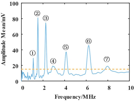
Figure 5.
Frequency–amplitude mean curve.
At the same time, combined with the classical threshold method, a smaller threshold method is introduced to filter WGN. The expression of the smaller threshold method is shown in (21).
In (21), N is the sampling data point and is the standard deviation of the signal. In order to ensure that the corresponding frequency peaks of the PD signal and the narrowband interference can be obtained at the same time, is usually taken as 0.1~0.5. Based on the large difference in the amplitude of the narrowband interference selected in this paper, is taken as 0.4. All narrowband interference frequency peaks and PD signal center frequency peaks can be obtained by a smaller threshold method.
In order to further distinguish the frequency of the two signals, the skewness of each peak frequency in Figure 5 is acquired, as shown in Table 3. From Table 3, it can be seen that the skewness value of peak points 1, 2, 3, 5 and 6 is less than 0, and it is determined that peak points 1, 2, 3, 5 and 6 correspond to the center frequency of narrowband interference, and the number of the narrowband interference is 5.
Table 3.
Skewness value of peak frequency.
4.2. Accurate Estimation of Narrowband Interference Frequency
In order to accurately estimate the frequency of narrowband interference, this paper introduces an improved Rife method based on the frequency–amplitude mean curve of FSWT [27].
The Rife method has high accuracy when the estimated frequency is located in the central region of two adjacent quantization frequencies, but the error may be larger than DFT when it is located near the quantization frequency point [28]. The improved Rife method uses the frequency shift technology to shift the signal frequency to the two adjacent quantized frequency center regions at one time, and then uses the Rife algorithm to estimate the frequency. The high precision and stable frequency estimation performance is obtained in the whole frequency band.
According to the principle of the improved Rife method, this paper moves the frequency of the original signal to δ approaching 0.5, and then the frequency of the signal after the frequency shift is accurately estimated by the Rife method, which reduces the estimation error of the whole frequency range. The algorithm is detailed as follows:
(1) In the frequency–amplitude mean curve of FSWT, the serial number corresponding to the peak spectral line of the narrowband interference frequency and the serial number of the sub-amplitude spectral line are obtained, and the amplitude corresponding to the spectral line is found: , .
(2) Calculate the correction value , as shown in (22).
(3) Obtain the estimated frequency of the narrowband interference. The calculation of is given by the following:
In (23), is the sampling frequency and is the number of sampling points.
(4) According to the estimated frequency , the frequency shift of the spectral line in and is carried out. The frequency shift distance is given in (24), and the peak value and of the spectral line in and after the frequency shift is obtained.
(5) Step (2) and Step (3) are carried out again to obtain the accurate frequency estimation of the narrowband interference signal.
This improved Rife method is used to estimate the narrowband interference frequency of the noisy PD signal in Figure 1c. The estimation results are shown in Table 4.
Table 4.
Results of narrowband interference frequency obtained by each method.
According to Table 4, the improved Rife method can estimate the narrowband interference frequency well. At the same time, its calculation is simple, enhancing efficiency and fitting for PD online monitoring.
4.3. SVD for Narrowband Interference Suppression
SVD is an important signal separation method. By singular value decomposition and selective reconstruction of the Hankel matrix of the noisy PD signal, the narrowband interference signal can be effectively suppressed. The specific steps are as follows:
(1) Set the noisy PD signal X according to the following:
In (26), n(k) is the periodic narrowband interference signal; p(k) is the PD signal; and k = 1, 2, …, N, N is the number of sampling points.
Construct Hankel matrix for sampling series X as follows:
Matrix A is a matrix of , and its rank is r.
(27) can be further expressed as:
In (28), is the PD signal subspace and is the narrowband interference subspace.
(2) Singular value decomposition of matrix A:
In (29), and are left and right orthogonal eigenvector matrices, respectively; and is a diagonal matrix, , where is the singular value of the matrix , which is arranged in descending order.
(3) Reconstruct the PD signal.
According to a large number of papers [18], narrowband interference signals correspond to large singular values, and each narrowband interference frequency corresponds to two non-zero singular values. Therefore, after obtaining the number m of narrowband interference from the frequency–amplitude mean curve of FSWT, narrowband interference suppression can be achieved by setting the first 2m singular values to zero. The reconstructed PD signal is shown in (30).
4.4. SVD with Guidance Signal
As the narrowband interference amplitude decreases, the corresponding singular value also decreases, and the aliasing area between the narrowband and PD subspaces in-creases, worsening the interference suppression effect. Therefore, how to realize the effective filtering of singular values corresponding to narrowband interference with small amplitude is also an important problem to be studied [29].
In order to ensure that the small amplitude narrowband interference in the SVD can still be accurately filtered out, this paper introduces the idea of increasing the narrowband interference amplitude by constructing the guidance signal from paper [29]. The specific steps of SVD with guidance signals are as follows:
(1) Perform FSWT on noisy PD signal X to adaptively obtain the number of narrowband interference m.
(2) Use the improved Rife method to accurately estimate the frequency of narrowband interference.
(3) Construct the guidance signal.
The expression of the guidance signal is shown in (31)
In (31), represents the maximum amplitude of the noise signal and represents the estimated frequency of the narrowband interference obtained by the improved Rife method.
(4) Add guidance signal g(t) to the noisy PD signal to obtain the mixed signal m(t), and m(t) is constructed within the Hankel matrix for SVD decomposition.
(5) Set the first 2m singular values to 0, and then the PD signal after narrowband interference suppression can be obtained by reconstructing the signal.
A noise reduction performance evaluation of traditional SVD methods and the proposed method for the noisy PD signal shown in Figure 1c is shown in Table 5, comparing the suppression effect of the narrowband interference by calculating the three indexes of SNR, NCC and RMSE. On this basis, the narrowband interference amplitude Ai in the noisy PD signal is transformed equally to verify its impact on the noise reduction method.
Table 5.
Noise reduction performance evaluation of different methods for different narrowband interference amplitude signals.
According to Table 5, ISVD is the most ideal in each evaluation index. The specific performance is as follows: the SNR of the noise-reduced PD signal is the largest, the NCC is the closest to 1 and the RMSE is the smallest, which represents the least residual noise content in the noise-reduced PD signal, the smallest error in amplitude and frequency and the highest similarity in waveform with the pure PD signal.
Additionally, as narrowband interference amplitude decreases, the traditional SVD method’s suppression effect worsens, while the proposed method in this paper remains effective.
5. MPA-Optimized MVMD and Improved Wavelet Threshold Noise Reduction Method
5.1. MPA for Parameter Optimization of MVMD
The second noise reduction uses MPA-optimized MVMD to decompose the noisy PD signal, filtering out narrowband interference and combining the 3σ criterion to obtain the reconstructed PD signal. The following is the MPA parameter setting:
(1) Selection of population size: The population size directly affects the search ability and computational efficiency of the MPA algorithm. The larger population size can increase the coverage of the search space, but it will also reduce the computational efficiency. After many experiments, the influence of different population sizes on the comprehensive performance of the optimization algorithm is compared. In this paper, the population size is 15.
(2) Determination of the search space boundary: The mode number k and the penalty factor α determine the accuracy of the decomposition and the bandwidth of the IMF component. The definition of the search space boundary is also extremely important. Paper [30] determined the value of k by observing the center frequency of each IMF decomposed of the cable partial discharge signal at different values (k = 2, 3, 4, 5, 6, 7). The results show that when the value of k is 6, the VMD algorithm effectively decomposes the frequency component of the PD signal and avoids decomposing too many high-frequency components. Considering the difference between the partial discharge signal model and its noise characteristics, in order to realize the full decomposition of the noisy partial discharge signal as much as possible, this paper sets the search space boundary of k as [2,15]. In paper [31], the sum of the kurtosis values of each IMF is used as the objective function, and the Beetle Antennae Search optimization algorithm is used to optimize the selection of the penalty factor. The results show that when k is 5, the penalty factor of the fifth-layer IMF component is 3850, which can decompose the PD characteristic signal most effectively. Considering the k value search space set in this paper, the search space boundary of the penalty factor is set as [100, 15,000].
(3) The determination of the number of modes k and the penalty factor value α: From Figure 4, it can be seen that with the increase in SNR, the average envelope entropy of the noisy PD signal gradually decreases. Therefore, with the minimum average envelope entropy value as the objective function, the noisy PD signal can decompose the PD characteristic signal with the greatest degree of certainty. Therefore, taking (15) as the objective function and using MPA to optimize the noisy PD signal, the optimal values of the modal number k and the penalty factor can be obtained.
The optimization results of MPA are shown in Figure 6. At the same time, the parameters of MVMD are optimized by particle swarm optimization (PSO) and the sparrow search algorithm (SSA), respectively. To guarantee the fairness of the experiment, the population size of the three algorithms is set to 15, the maximum number of iterations is set to 20, the search space of the modal number k is [2, 15] and the search space of the quadratic penalty factor α is [100, 15,000]. The two parameters of the individual learning factor and the social learning factor of the PSO algorithm are set to 1.5; the warning value of SSA is ST = 0.7, and the number of discoverers and alerters is 30% and 50% of the population size, respectively. The effect coefficient of the fish aggregation device in MPA is set to 0.2.
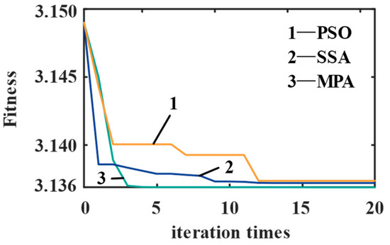
Figure 6.
Optimization results of different optimal algorithms.
From Figure 6, the MAEE of MPA is 3.1369, which appears in the sixth generation. After searching, the parameter k is 6, and the parameter α is 6981. Therefore, k in MVMD is set to 6, while α is set to 981. The input parameters are used to perform MVMD decomposition on the PD signal that filters out narrowband interference signals.
In addition, the SSA algorithm converges faster than the PSO algorithm, but the SSA algorithm is falls easily into the local optimum. The PSO algorithm has strong global search ability, but the convergence speed is slow. The MPA algorithm has a small number of iterations, a fast convergence speed and strong global search ability, and its optimization results are closer to the global optimal value. In summary, the optimization ability of the MPA algorithm is better than that of the PSO algorithm and SSA algorithm. Using MPA to optimize the core parameters of MVMD can significantly reduce the subjectivity of the decomposition structure and improve the decomposition effect.
5.2. Improvement of Wavelet Threshold Noise Reduction
The third noise reduction denoises the reconstructed PD signal via the improved wavelet threshold algorithm to obtain the final denoised PD signal. The improved wavelet threshold algorithm is shown as follows:
(1) The selection of wavelet basis: Selecting the appropriate wavelet basis can effectively extract the characteristics of PD signals. According to paper [32], the threshold noise reduction method based on the db7 wavelet has a good noise reduction effect on the field data, and the db7 mother wavelet is very similar to the PD pulse current signal collected by the high-frequency current sensor. In addition, paper [33] gives the maximum NCC value and corresponding SNR of four PD simulation signals under dbN (N = 2, 3, …,12) noise reduction. The results show that db7 has better noise reduction performance for four PD simulation signals. Therefore, the db7 wavelet is selected as the wavelet basis function in this paper.
(2) Selection of decomposition scale: The noisy PD signal from Figure 1c is used, and the SNR is set to 4 dB. The SNR value of the noise-reduced signal under different decomposition layers is calculated. When the decomposition layers are taken as 1, 2, 3, 4, 5, 6, 7, 8 and 9, respectively, the SNR value of the noise-reduced signal is 6.404, 8.632, 9.826, 10.239, 10.762, 11.077, 11.120, 11.178 and 11.056. According to this trend, it can be seen that the noise reduction signal has the highest SNR when the decomposition scale is eight. Therefore, the eight-layer db7 wavelet decomposition method is selected in this paper.
(3) The improvement of the wavelet threshold and the threshold function: The improved threshold is shown in (32).
In (32), is the improved wavelet threshold, N is the number of sampling points, σ is the standard deviation of the noisy PD signal and represents the number of wavelet decomposition layers.
It can be seen that wavelet decomposition layer i is introduced into the wavelet threshold so that the PD signal at each level can be better extracted. The improved threshold function is expressed in (33).
In the formula, is the wavelet coefficient and is the improved wavelet coefficient.
For the purposes of comparing the characteristics of the improved threshold function and the soft and hard threshold function, is taken, as shown in Figure 7.
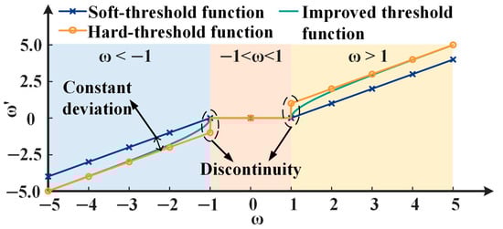
Figure 7.
Comparison of three threshold functions.
Figure 7 shows that after the hard threshold function is processed, there is a discontinuity at , which makes the noise-reduced signal oscillate and lack the smoothness of the original signal. After the soft threshold function is processed, although it is continuous at , there is a large constant deviation between the processed signal and the original signal. The improved threshold function can quickly approach the hard threshold function, while overcoming the discontinuity of the hard threshold function and the constant deviation of the soft threshold function. The exponential attenuation wavelet threshold function is suitable for the PD signal waveform, which is helpful for extracting the features of the PD signal.
The comparison of different threshold functions for the noisy PD signal can be seen in Figure 8. The evaluation index can be seen in Table 6.
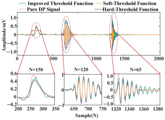
Figure 8.
Noise reduction results of different threshold functions.
Table 6.
Noise-reduced performance evaluation of different threshold functions.
According to Figure 8, the improved threshold function has the best noise reduction effect on the PD signal. The noise-reduced PD signal is most similar to the pure PD signal, with the smallest amplitude error and less residual noise. The PD signal obtained by the soft threshold function and hard threshold function has a large amplitude error and a certain degree of distortion.
In Table 6, the signal obtained via the improved threshold function has the largest SNR and NCC value and the smallest RMSE value. Obviously, the improved threshold function is superior to the other two threshold functions.
6. Simulation and Analysis
The process of the overall noise reduction method in this paper is shown in Figure 9.
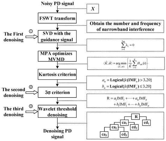
Figure 9.
Flow chart of the overall noise reduction method in this paper.
Based on Figure 9, The noise reduction methods in this paper are detailed as follows:
Step (1): The amount of narrowband interference is adaptively determined by the FSWT frequency–amplitude mean graph. If the number of the narrowband interference is 0, the second step is skipped and the third step is performed.
Step (2): The narrowband interference frequency is determined by the improved Rife method. On the basis of determining the amount and frequency of narrowband interference, the guidance signal is constructed, and the guidance signal is added to the noisy PD signal. The narrowband interference signal is filtered by setting the singular value to zero, and the obtained waveform is shown in Figure 10. According to Figure 10, the ISVD method can better suppress the narrowband interference signal.
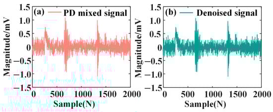
Figure 10.
Noise reduction results of narrowband interference. (a) PD mixed signal without adding narrowband interference; (b) signal after noise reduction from narrowband interference.
Step (3): After the optimal mode number k and penalty factor α are optimized by MPA, the PD signal (filtered narrowband interference) is decomposed with MVMD, and the obtained IMFn waveform can be seen in Figure 11. According to Figure 11, the MVMD algorithm can effectively extract the waveform characteristics of the PD signal, and the obtained IMFn component has good physical meaning.
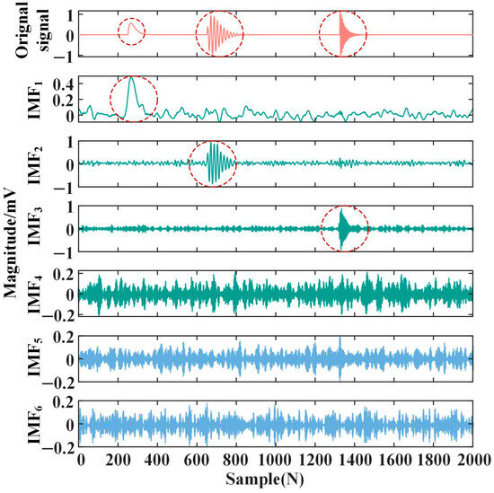
Figure 11.
IMFn of the noisy PD signal.
Step (4): The kurtosis of each modal component of IMF1 ~ IMF6 is calculated, respectively, as shown in Table 7.
Table 7.
Kurtosis value of imfn.
From Table 7, the kurtosis values of IMF1–IMF4 are greater than 3.2; others are less than the threshold. Therefore, IMF1–IMF4 are classified as PD characteristic information.
Step (5): According to the size of the kurtosis, the characteristics of the modal components are determined. According to the calculation results, IMF1–IMF4 are the PD-dominant components, while IMF5 and IMF6 are the noise-dominant components. Therefore, the 3σ criterion is used to filter IMFn from the noise-dominant components. The filtering results are shown in Figure 12. It can be seen from Figure 12 that the 3σ criterion preserves the gross error belonging to the PD signal and basically suppresses the WGN and narrowband interference signals.
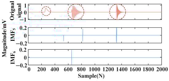
Figure 12.
The filtering results of the 3σ criterion.
Step (6): The reconstructed PD signal R is obtained by adding the noise-dominant component after filtering via the 3σ criterion and the PD characteristic information. The calculation of R is shown in (34).
In (34), , and , where is a logical judgment function, which satisfies the condition to return 1; is the calculation of kurtosis; is the standard deviation of IMFn; and is the mean value of IMFn.
Step (7): The improved wavelet threshold function is used to denoise R, and the noise-reduced PD signal is obtained.
In addition, the noise reduction effects of noisy PD analog signals under the same conditions are compared via Spearman Variational Mode Decomposition (S_VMD) [13], Image Information Entropy and MVMD (IIE-MVMD) [14], and SVD and EWT [18].
According to the principles of each method, S_VMD and IIE-MVMD do not add narrowband interference suppression steps. Though SVD-EWT can suppress narrowband interference, its effect is weak when the interference amplitude is low. Thus, the proposed method in this paper has unique advantages in narrowband interference suppression.
In addition, the modal parameter k of VMD in S_VMD only considers the thoroughness of decomposition and does not consider the accurate extraction of PD feature signals. IIE-MVMD deeply considers the setting of modal parameter k, but the penalty factor α still uses a fixed empirical value. In this paper, the MPA algorithm considering the MAEE is adopted, which can extract the characteristics of PD pulse signals to the greatest extent on the basis of adaptively obtaining k and α values. SVD-EWT adopts the noise reduction strategy of truncating and retaining PD. Though this strategy can maximally remove white noise, precisely locating PD start and end positions is challenging, and its noise reduction reliability needs further consideration. Finally, the improved wavelet threshold method proposed in this paper can eliminate white noise to the greatest extent on the basis of retaining the PD characteristic signal.
The results of different methods can be seen in Figure 13.
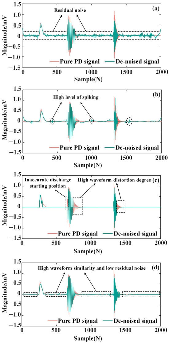
Figure 13.
Noise reduction results of different methods in Simulated PD signals. (a) S_VMD; (b) IIE-MVMD; (c) SVD-EWT; (d) ISVD-MVMD.
According to Figure 13, the residual noise content of the signal denoised by S_VMD is large, and the noise reduction effect is not ideal. The noise reduction effect of IIE-MVMD is obviously improved, but there is still some spiking. Although SVD-EWT is used to segment and denoise the PD signal, and the removal effect of residual noise is significant, the starting position of the PD signal has shifted to a certain extent, which will affect the diagnosis and evaluation of defects. ISVD-MVMD can make the noise-reduced PD signal and the pure PD signal keep the waveform consistent as much as possible; the residual noise content is small, so the PD signal can eliminate narrowband interference and WGN as much as possible without distortion.
The spectrograms of a pure PD signal and a PD signal denoised by the above four methods are obtained, respectively, as shown in Figure 14.
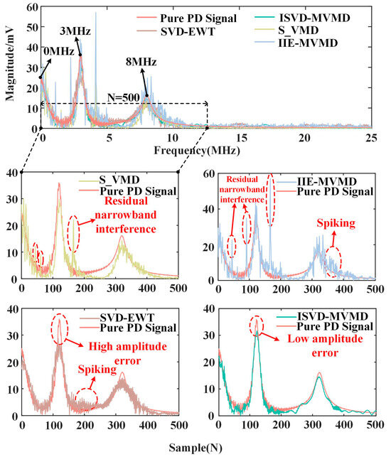
Figure 14.
Spectrum analysis after noise reduction of the PD signals.
In Figure 14, the useful information of the PD signal is mainly concentrated at 0 Hz, 3 MHz and 8 MHz. S_VMD and IIE-MVMD retain the waveform characteristics of the pure PD signal more completely, but the suppression effect on narrowband interference and WGN is general. SVD-EWT successfully suppresses narrowband interference by singular value decomposition, and the noise reduction effect on WGN is also good, but the PD signal has certain distortion and a large amplitude error. ISVD-MVMD successfully suppresses the periodic narrowband interference and WGN of the PD signal, and in the spectrum distribution, the distribution of the noise-reduced PD signal is basically the same as that of a pure PD signal.
Through the calculation of the three indicators of SNR, NCC and RMSE, the noise reduction effects of the above four methods are further compared. The results can be seen in Table 8.
Table 8.
Noise reduction performance evaluation of different methods.
It can be seen from Table 8 that the evaluation indexes of ISVD-MVMD are the most ideal. The SNR value of the noise-reduced PD signal is the largest, at about 13.0791, the NCC value is the closest to 1, at about 0.9769, and the RMSE value is the closest to 0, at about 0.0326.
Furthermore, in order to evaluate the running efficiency of the proposed algorithm, the running efficiency index of the algorithm is constructed by SNR, NCC, RMSE and algorithm duration, as shown in (35). For the field-measured PD signal, the algorithm operation efficiency index is constructed by NRR, ARR and algorithm duration, as shown in (36). The time-consuming and operating efficiency indicators of different algorithms are shown in Table 9.
Table 9.
Comparison of duration and operating efficiency indicators of Simulated PD signals for different algorithms.
From Table 9, it can be seen that the algorithm time of this method is smaller than that of the S_VMD method and slightly larger than that of the IIE-MVMD method and SVD-EWT method. However, due to the good noise reduction performance, the algorithm efficiency of this method is obviously better than the other algorithms.
For the purposes of studying the noise reduction effect of ISVD-MVMD on the noisy PD signal under different SNRs, WGN with SNRs of −3, 0 and 3 dB and narrowband pulses with the same parameters are superimposed on the pure PD signal shown in Figure 1a. Through the calculation of SNR, NCC and RMSE, the noise reduction effects of the above four methods are further compared. The results are shown in Table 10.
Table 10.
Noise reduction performance evaluation under different SNRs.
According to Table 10, the three indicators of ISVD-MVMD perform best under WGN with different SNRs.
7. Field Test
To further verify the effectiveness of the proposed method in reducing the noise of field PD signals, the proposed method is used to denoise the PD signals measured in the field, and the results are compared with S_VMD, IIE-MVMD and SVD-EWT.
7.1. Online Monitoring System Based on the Pulse Current Method
The online monitoring system based on the pulse current method is composed of a high-frequency current transformer (HFCT), a signal conditioning module, a high-frequency acquisition module and an industrial computer. The schematic diagram of the system is shown in Figure 15. By installing an HFCT on the cable grounding line to collect the partial discharge current pulse signal, the signal output via an HFCT is transmitted to the signal conditioning module through the high-frequency double-shielded coaxial cable for filtering and amplification. The signal is sent to the industrial computer through the high-speed data acquisition card for signal processing and analysis. Among them, the current transformer uses a broadband high-frequency current transformer produced by a company in Xi’an, with a maximum bandwidth of 100 Mhz. The acquisition card uses a QT7126 board, and the upper limit of the sampling rate is 3.2 GS/s. Some field devices are shown in Figure 16.
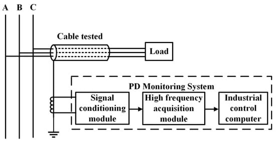
Figure 15.
Online monitoring system diagram.
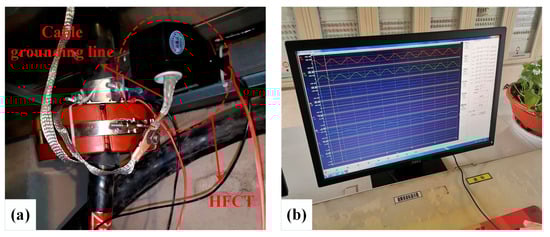
Figure 16.
Field monitoring equipment. (a) HFCT; (b) industrial control computer.
7.2. Field-Measured PD Signal
A 6 kV MYJV cross-linked polyethylene cable with a length of about 250 m from a 110 kV substation to a coal-washing plant in a coal mine in Shanxi Province was detected as having partial discharge. The field-measured PD signal can be seen in Figure 17a. With the aim of fully verifying the noise reduction effect of different methods, multiple narrowband interference signals with amplitudes of 0.5 mV, 1 mV and 1.5 mV and frequencies of 1 MHz, 1.5 MHz and 2.2 MHz are added, as shown in Figure 17b.
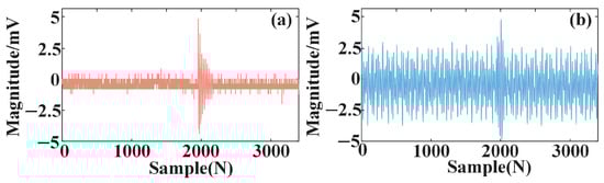
Figure 17.
Field data. (a) Field-measured PD signal; (b) field-measured PD signal with narrowband interference.
S_VMD, IIE-MVMD, SVD-EWT and ISVD-MVMD are applied to denoise the field-measured signal, and the noise reduction results can be seen in Figure 18.
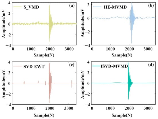
Figure 18.
Noise reduction results of different methods in field-measured PD signals. (a) S_VMD; (b) IIE-MVMD; (c) SVD-EWT; (d) ISVD-MVMD.
According to Figure 18, there is still residual noise after noise reduction by S_VMD, which will affect the defect diagnosis and location of subsequent cables. The waveform residual noise after noise reduction by IIE-MVMD and SVD-EWT is small, but the PD signal waveform distortion is more serious. After noise reduction by ISVD-MVMD, the WGN and narrowband interference signals can be suppressed to the greatest extent, and the PD waveform characteristics after noise reduction are obvious.
The calculation results of the NRR and the ARR of the field-measured PD signal can be seen in Table 11.
Table 11.
Noise reduction performance evaluation of field-measured data.
According to Table 11, the NRR value of the PD signal denoised by ISVD-MVMD is 4.5008, which is the largest among different noise reduction methods. This shows that the PD signal obtained by ISVD-MVMD has the least residual noise content. The ARR value is 0.2017, which is only slightly larger than the SVD-EWT. However, compared with SVD-EWT, ISVD-MVMD retains the waveform characteristics of the PD signal completely, and the PD signal is easy to identify. The high NRR value and the low ARR value indicate that the noise reduction effect is good. Therefore, this method is also superior to the noise reduction effect of the actual collected PD signal in the field measurement. The time-consuming and operating efficiency indicators of the algorithm are shown in Table 12.
Table 12.
Comparison of duration and operating efficiency indicators of field-measured PD signals for different algorithms.
It can be seen from Table 12 that the algorithm time of this method is close to that of the IIE-MVMD method and the SVD-EWT method, which is much smaller than that of the S_VMD method. Through the construction of the algorithm operation efficiency index, the algorithm operation efficiency of this method is the highest, which has certain advantages for the noise reduction situation with a large amount of data.
8. Conclusions
In this paper, ISVD and MVMD for PD signal noise reduction are proposed. Through the analysis of the simulated and field-measured signals, the effect of the noise reduction method in this paper is verified, and the following conclusions are drawn:
(1) The SVD algorithm with a guidance signal is proposed. The elements of the guidance signal are adaptively obtained by FSWT and the improved Rife method, and the guidance signal is added to the noisy PD signal to complete the narrowband interference suppression. At the same time, the various indicators of this method are better than the traditional SVD narrowband interference suppression method, even in the case of small narrowband interference amplitude.
(2) MPA considering MAEE is used to realize the automatic optimization of MVMD modal decomposition number k and penalty factor α. The optimal decomposition of the noisy PD signal is realized, and the modal aliasing phenomenon is overcome. PD feature information can be accurately extracted to improve the accuracy of PD detection.
(3) Through the wavelet threshold introduced by decomposition layer i and the new exponential attenuation threshold function, the fitting effect of the PD signal is enhanced and a better noise reduction effect is achieved. Through the noise reduction of simulated and field PD signals, the SNR, NCC and RMSE indexes of the overall noise reduction method in this paper are better than SVMD, IIE-MVMD and SVD-EWT, and the efficiency of the algorithm is the best.
Although the method proposed in this paper has better noise reduction performance, the algorithm takes a long time. The complexity of the algorithm will be further improved in the future, thus reducing the time consumption of the algorithm.
Author Contributions
Conceptualization, J.C. and Y.W.; Methodology, J.C., Y.W., W.Z. and Y.Z.; Software, W.Z. and Y.Z.; Validation, W.Z. and Y.Z.; Writing—original draft, J.C.; Writing—review & editing, J.C.; Supervision, Y.W.; Funding acquisition, Y.W. All authors have read and agreed to the published version of the manuscript.
Funding
This work was supported in part by “the Fundamental Research Funds for the Central Universities (Ph.D. Top Innovative Talents Fund of CUMTB)”, and in part by the National Natural Science Foundation of China under Grant 52474188.
Institutional Review Board Statement
Not applicable.
Informed Consent Statement
Not applicable.
Data Availability Statement
The original contributions presented in this study are included in the article. Further inquiries can be directed to the corresponding author.
Conflicts of Interest
The authors declare no conflict of interest.
References
- Shams, M.A.; Anis, H.I.; El-Shahat, M. Denoising of Heavily Contaminated Partial Discharge Signals in High-Voltage Cables Using Maximal Overlap Discrete Wavelet Transform. Energies 2021, 14, 6540. [Google Scholar] [CrossRef]
- Chen, J.; Yan, Y.; Zhao, K.; Zhu, M.; Wang, L.; Lu, Y.; Hou, Z.; Li, H. Improved Double-Sided Partial Discharge Location Method for High-Voltage Cables via Pulse-Injected Time Synchronization and Variational Mode Decomposition. IEEE Trans. Instrum. Meas. 2025, 74, 3504315. [Google Scholar] [CrossRef]
- Wang, Y.; Chen, P.; Zhao, Y.; Sun, Y. A Denoising Method for Mining Cable PD Signal Based on Genetic Algorithm Optimization of VMD and Wavelet Threshold. Sensors 2022, 22, 9386. [Google Scholar] [CrossRef]
- Zhong, J.; Liu, Z.; Bi, X. Partial Discharge Signal Denoising Algorithm Based on Aquila Optimizer–Variational Mode Decomposition and K-Singular Value Decomposition. Appl. Sci. 2024, 14, 2755. [Google Scholar] [CrossRef]
- Hua, X.-C.; Mu, H.-B.; Jin, L.-F.; Ji, Y.-H.; Zhan, J.-Y.; Shao, X.-J.; Zhang, G.-J. A Novel Adaptive Parameter Optimization Method for Denoising Partial Discharge Ultrasonic Signals. IEEE Trans. Dielectr. Electr. Insul. 2023, 30, 2734–2743. [Google Scholar] [CrossRef]
- Xu, H.; Zhu, X.; Jiang, X.; Geng, H.; Ayubi, B.I.; Zhang, L. Equilibrium Optimizer-Based Variational Mode Decomposition Method for Partial Discharge Denoising. In Proceedings of the 2022 4th International Conference on Smart Power & Internet Energy Systems (SPIES), Beijing, China, 9–12 December 2022; pp. 1289–1294. [Google Scholar]
- Jiang, T.; Yang, X.; Yang, Y.; Chen, X.; Bi, M.; Chen, J. Wavelet method optimised by ant colony algorithm used for extracting stable and unstable signals in intelligent substations. CAAI Trans. Intell. Technol. 2021, 7, 292–300. [Google Scholar] [CrossRef]
- Ghorat, M.; Gharehpetian, G.B.; Latifi, H.; Hejazi, M.A. A New Partial Discharge Signal Denoising Algorithm Based on Adaptive Dual-Tree Complex Wavelet Transform. IEEE Trans. Instrum. Meas. 2018, 67, 2262–2272. [Google Scholar] [CrossRef]
- Tang, J.; Zhou, S.; Pan, C. A Denoising Algorithm for Partial Discharge Measurement Based on the Combination of Wavelet Threshold and Total Variation Theory. IEEE Trans. Instrum. Meas. 2020, 69, 3428–3441. [Google Scholar] [CrossRef]
- Sahnoune, M.A.; Zegnini, B.; Seghier, T.; Flah, A.; Kanan, M.; Prokop, L.; El-Bayeh, C.Z. Noise Source Effect on the quality of Mother Wavelet Selection for Partial Discharge Denoising. IEEE Access 2024, 12, 132729–132743. [Google Scholar] [CrossRef]
- Zhong, J.; Bi, X.; Shu, Q.; Zhang, D.; Li, X. An Improved Wavelet Spectrum Segmentation Algorithm Based on Spectral Kurtogram for Denoising Partial Discharge Signals. IEEE Trans. Instrum. Meas. 2021, 70, 3514408. [Google Scholar] [CrossRef]
- Jin, T.; Li, Q.; Mohamed, M.A. A Novel Adaptive EEMD Method for Switchgear Partial Discharge Signal Denoising. IEEE Access 2019, 7, 58139–58147. [Google Scholar] [CrossRef]
- Xh, M.; Kong, W.D.; Li, Z.Q.; Wang, W.S.; Bao, J.W. A denoising method for a partial discharge signal based on S_VMD and Sdr_SampEn. Power Syst. Prot. Control 2022, 50, 29–38. [Google Scholar]
- Wang, X.; Wang, X.; Gao, J.; Tian, Y.; Kang, Q.; Zhang, F.; Liu, W. A Denoising Method for Cable Partial Discharge Signals Based on Image Information Entropy and Multivariate Variational Mode Decomposition. IEEE Trans. Instrum. Meas. 2024, 73, 3500415. [Google Scholar] [CrossRef]
- Ashtiani, M.; Shahrtash, S. Partial discharge de-noising employing adaptive singular value decomposition. IEEE Trans. Dielectr. Electr. Insul. 2014, 21, 775–782. [Google Scholar] [CrossRef]
- Abdel-Galil, T.K.; El-Hag, A.H.; Gaouda, A.M.; Salama, M.M.A.; Bartnikas, R. De-noising of partial discharge signal using eigen-decomposition technique. IEEE Trans. Dielectr. Electr. Insul. 2008, 15, 1657–1662. [Google Scholar] [CrossRef]
- Lei, Z.; Wang, F.; Li, C. A Denoising Method of Partial Discharge Signal Based on Improved SVD-VMD. IEEE Trans. Dielectr. Electr. Insul. 2023, 30, 2107–2116. [Google Scholar] [CrossRef]
- Zhong, J.; Bi, X.; Shu, Q.; Chen, M.; Zhou, D.; Zhang, D. Partial Discharge Signal Denoising Based on Singular Value Decomposition and Empirical Wavelet Transform. IEEE Trans. Instrum. Meas. 2020, 69, 8866–8873. [Google Scholar] [CrossRef]
- Xu, Y.; Jiang, J.; Tang, K.; Zhang, T.; Luo, J.; Xie, M. A Method of Suppressing Narrow-band Interference in Partial Discharge Based on Hankel Matrix and Singular Value Decomposition. Power Syst. Technol. 2020, 44, 2762–2769. [Google Scholar]
- Wang, S.; He, Y.; Yin, B.; Zeng, W.; Li, C.; Ning, S. Multi-Resolution Generalized S-Transform Denoising for Precise Localization of Partial Discharge in Substations. IEEE Sens. J. 2021, 21, 4966–4980. [Google Scholar] [CrossRef]
- Wu, Z.; Zhang, Z.; Zheng, L.; Yan, T.; Tang, C. The Denoising Method for Transformer Partial Discharge Based on the Whale VMD Algorithm Combined with Adaptive Filtering and Wavelet Thresholding. Sensors 2023, 23, 8085. [Google Scholar] [CrossRef] [PubMed]
- Chaudhuri, S.; Ghosh, S.; Dey, D.; Munshi, S.; Chatterjee, B.; Dalai, S. Denoising of partial discharge signal using a hybrid framework of total variation denoising-autoencoder. Measurement 2023, 223, 113674. [Google Scholar] [CrossRef]
- Yan, Z.; Miyamoto, A.; Jiang, Z.; Liu, X. An overall theoretical description of frequency slice wavelet transform. Mech. Syst. Signal Process. 2010, 24, 491–507. [Google Scholar] [CrossRef]
- Zhang, Y.; Liu, M.; Huang, N. Application of Frequency Slice Wavelet Transform in Partial Discharge Signal Analysis. High Volt. Eng. 2015, 41, 2283–2293. [Google Scholar]
- Liu, S.B.; Lu, C.; Yu, J.L.; Wang, L.X. Application of Hilbert-Huang Transform in Pattern Recognition for Partial Discharge of Transformers. Proc. CSEE 2008, 28, 114–119. [Google Scholar]
- Faramarzi, A.; Heidarinejad, M.; Mirjalili, S.; Gandomi, A.H. Marine Predators Algorithm: A nature-inspired metaheuristic. Expert Syst. Appl. 2020, 152, 113377. [Google Scholar] [CrossRef]
- Wang, H.; Zhao, G. Improved Rife Algorithm for Frequency Estimation of Sinusoid Wave. Signal Process. 2010, 26, 1573–1576. [Google Scholar]
- Rife, D.; Boorstyn, R. Single tone parameter estimation from discrete-time observations. IEEE Trans. Inf. Theory 1974, 20, 591–598. [Google Scholar] [CrossRef]
- Rao, X.; Zhou, K.; Wang, X.; Li, M.; Huang, Y.; Xie, M. Suppression of Narrow-band Noise of Partial Discharge Based on Improved SVD Algorithm. High Volt. Eng. 2021, 47, 705–713. [Google Scholar]
- Ma, X.; Zhu, H.; Liu, Z.; Zhang, D. An adaptive threshold value noise suppression method for detecting partial discharge of power cables based on variational mode decomposition. Power Syst. Prot. Control 2019, 47, 145–151. [Google Scholar]
- Xiao, S.; Chen, B.; Shen, D.; Chen, H. Application of improved VMD and threshold algorithm in partial discharge denoising. J. Electron. Meas. Instrum. 2021, 35, 206–214. [Google Scholar]
- Mei, L.; Quan, H. A Study on the Online Insulation Monitoring System for High Voltage Cables Based on Double CPUs. J. Chongqing Electr. Power Coll. 2017, 22, 20–23, 44. [Google Scholar]
- Wan, L.; Zhang, X.; Xie, Y.; Tang, J. Constructing dbN complex wavelets for PD signal denoise. Electr. Power Autom. Equip. 2007, 19–23, 37. [Google Scholar] [CrossRef]
Disclaimer/Publisher’s Note: The statements, opinions and data contained in all publications are solely those of the individual author(s) and contributor(s) and not of MDPI and/or the editor(s). MDPI and/or the editor(s) disclaim responsibility for any injury to people or property resulting from any ideas, methods, instructions or products referred to in the content. |
© 2025 by the authors. Licensee MDPI, Basel, Switzerland. This article is an open access article distributed under the terms and conditions of the Creative Commons Attribution (CC BY) license (https://creativecommons.org/licenses/by/4.0/).