Controlled Fault Current Interruption Scheme for Improved Fault Prediction Accuracy

Abstract

To enhance the accuracy and efficiency of controlled fault current interruption (CFI) in short-circuit current processing within power systems, a half-cycle elimination prediction algorithm and a double-sampling CFI sequence method are proposed in this study. By analyzing the non-periodic and periodic components of short-circuit currents, the half-cycle elimination method and fast Fourier transform are utilized to compute these two components, respectively. The double-sampling CFI sequence approach is designed to fully utilize the response and waiting times of relay protection. Following the first sampling to estimate the target zero-crossing point, the remaining response and waiting times are allocated for a second sampling and recalculation to enhance the precision of zero-crossing prediction. MATLAB R2023a is employed to conduct multi-scenario simulations, and the algorithm’s performance is evaluated using actual recorded waveform data. The results demonstrate that the proposed algorithm accurately predicts the target zero-crossing point after a short circuit, with a computational error of less than 0.2 ms. Furthermore, the double-sampling sequence method is shown to improve the accuracy of open-circuit zero-crossing point calculations by an order of magnitude. This work provides a novel technical approach for the fast and precise handling of short-circuit faults in power systems.

1. Introduction

Among the various types of power system faults, short-circuit accidents are the most prominent. This abnormal state will produce a short-circuit current far in excess of the rated value, and the thermal effect and arcing phenomenon triggered by it have significant destructive power. Especially noteworthy is the fact that the instantaneous release of the fault point of a huge amount of energy will not only cause permanent damage to the electrical device, but will likely cause fire and other secondary disasters. Therefore, short-circuit faults are a key type of accident to prevent in the field of industrial safety [1,2]. In addition, the repulsive electromagnetic forces generated by short-circuit currents can cause serious damage to power equipment, especially transformers, resulting in radial and axial insulation damage, bushing failure, and tank rupture [3,4,5]. In current industry practice, short-circuit faults are mainly predicted by transient characteristics, and some restrictive measures are taken to reduce the hazards of short-circuit faults [6,7]. When a short circuit occurs in a power system, the current will rise to ten or even hundreds of times its original value in a few microseconds, jeopardizing the safe operation of the power system [8,9]. Therefore, it is of great significance to quickly and accurately calculate the short-circuit current parameters and predict the short-circuit current over the zero point to complete the CFI (controlled fault current interruption) to ensure the safe and stable operation of the power system, as well as to reduce the damage caused by short-circuit faults [10,11]. In addition, there are interference problems, such as noise and harmonics in the actual power system, that also test the anti-harmonic and anti-noise abilities of the prediction algorithm [12].

Research on predicting short-circuit current crossing points by identifying short-circuit current waveform parameters is scarce, and most studies have limitations. The authors of [13,14] used the least squares method to identify the short-circuit current parameters, but the algorithm ignores the effect of harmonic factors and has a large error. The study in [15] used an improved half-wave Fourier algorithm to process the current signal, but the algorithm does not take into account the effect of noise in testing and does not have a practical application value. The study in [16] proposes a safe point algorithm, which reacts quickly but does not take into account the attenuation of the DC component of the fault current. The current model is too simple and the over-zero point prediction accuracy is low. The authors of [17] propose an LSTM-based short-circuit current over-zero prediction method, but the calculation time of this method is too long and cannot meet the requirements of response speed in the field.

In this paper, we propose an innovative half-cycle elimination method combining RLS (recursive least squares) and FFT (fast Fourier transform) to meet the stringent requirements of CFI for computational accuracy and speed. The core of the method lies in the utilization of the property that the values of sinusoidal functions are opposite to each other when the phase difference is half a cycle, which determines the independent identification of the parameters of the non-periodic component and the periodic component of the short-circuit current. Specifically, this paper adopts the RLS method to calculate the parameters of the non-periodic components in real time, so as to determine the real-time prediction of the short-circuit current, while the periodic components are calculated using FFT. The advantages of the recursive least squares method can be fully utilized, i.e., it is good at fitting linear data, and of the fast Fourier algorithm, which is good at calculating sinusoidal quantities. The algorithm is tested in MATLAB using simulation data and recorded waveform data, and the results show the advantages of the algorithm in terms of accuracy.

After successfully calculating the target breaking point, the sequence of CFI is the key to realize the controlled switching of the short-circuit current. The CFI sequence adopted in most of the current studies is relatively simple, and the main idea is to pre-calculate the opening zero-crossing point before the relay protection action and to determine the waiting time by combining the breaking time with the arc ignition time [18]. However, this type of sequence often does not fully utilize the relay protection response time and waiting time. To address this problem, this paper proposes a double-sampling controlled switching sequence. The first calculation is completed before the relay protection response time, and the target zero-crossing point is obtained through the first sampling calculation. Secondly, on the basis of retaining a certain degree of redundancy, the short-circuit current is continued to be sampled and calculated by utilizing the remaining relay protection response time and waiting time to improve the accuracy of the calculation of the target zero-crossing point, which is obtained in the final iteration result, before finally being combined with the breaking time and the arcing time to calculate the breaking signal issuance time to complete the CFI.

Finally, the method proposed in this paper is compared with articles applying least squares and Fourier algorithms, and the results can fully prove the superiority of the method and sequence.

2. Short-Circuit Current Prediction Algorithm

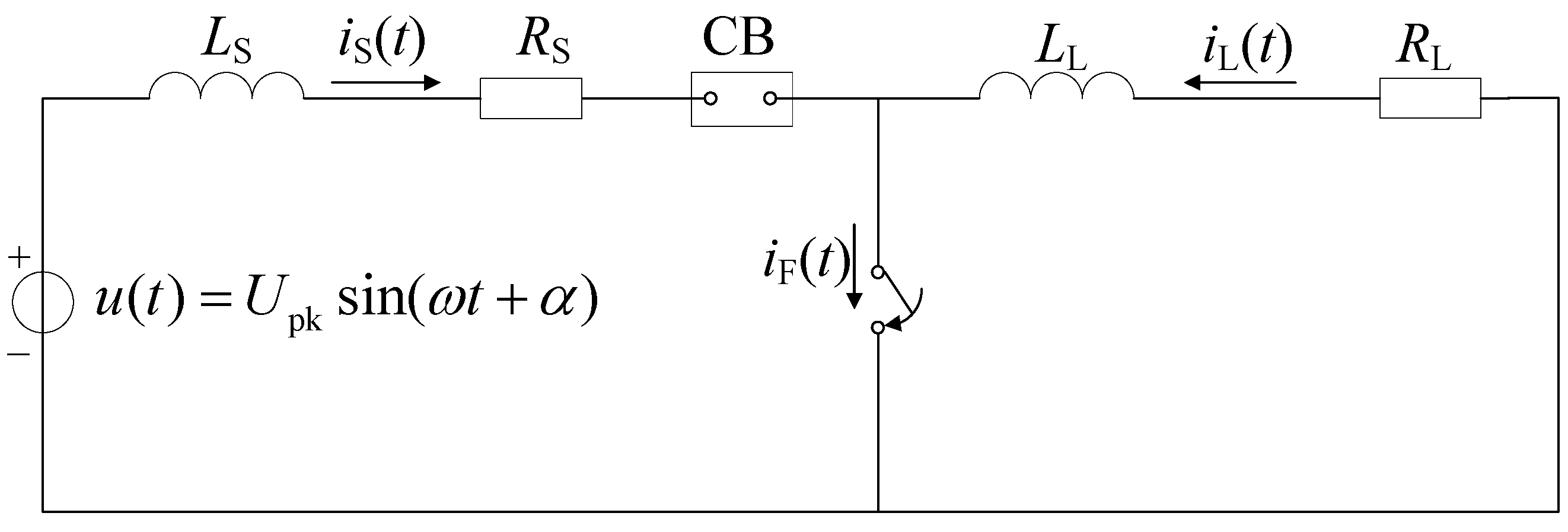
2.1. Short-Circuit Current Model

The short-circuit situation in a high-voltage power system can be analyzed equivalently using a single-phase short-circuit fault model, as shown in Figure 1.

In the figure, CB is the circuit breaker; $u(t)$ is the voltage of the ideal voltage source; $U_{\mathrm{pk}}$ is the peak voltage; $\omega$ is the angular frequency; $\alpha$ is the phase angle of the voltage at the moment of short circuit; $j\omega L_S+R_S$ is the fault impedance of the power supply side; $j\omega L_{\mathrm{L}}+R_{\mathrm{L}}$ is the fault impedance of the load side; $i_s(t)$ is the short-circuit current of the supply side; $i_{\mathrm{L}}(t)$ is the short-circuit current of the load side; and $i_{\mathrm{F}}(t)$ is the short-circuit current to ground.

If a short-circuit occurs at the moment t = 0, by applying both Kirchhoff’s law and the Rasch transform, the time-domain expression for the short-circuit current on the power supply side can be found as follows [19,20]:

$$i_{\mathrm{s}}(t)=X_1\cdot \sin \left(\omega t+X_2\right)+X_3\cdot {\mathrm{e}}^{-{\displaystyle \frac{t}{X_4}}}$$

(1)

Among

$$\left\{\begin{array}{l}{X}_1=I_{\mathrm{pk}}\\ X_2=\alpha -\varphi \\ X_3=i(0)-I_{\mathrm{pk}}\cdot \sin (\alpha -\varphi )\\ X_4=\tau \end{array}\right.$$

(2)

Equation (1) can be viewed as a superposition of the periodic component $I_{\mathrm{pk}}\cdot \sin (\omega t+\alpha -\varphi )$ and the non-periodic component $\left[i(0)-I_{\mathrm{pk}}\cdot \sin (\alpha -\varphi )\right]\cdot {\mathrm{e}}^{-t/\tau }$, where $i(0)$ is the current value at the initial moment of the fault, $\tau$ is the time constant of the faulted circuit, and $\varphi$ is the voltage–current phase difference.

If the effect of the third and fifth harmonics in the grid is considered, the short-circuit current coefficient expression is as follows:

$$\begin{array}{cc}\hfill i(t)& =X_1\cdot \sin \left(\omega t+X_2\right)+X_3\cdot {\mathrm{e}}^{-{\displaystyle \frac{t}{X_4}}}\hfill \\ & +X_5\cdot \sin \left(3\omega t+X_6\right)\\ & +X_7\cdot \sin \left(5\omega t+X_8\right)\end{array}$$

(3)

2.2. Half-Cycle Elimination Method

In the short-circuit current expression, the period component is a sinusoidal function. According to the properties of sinusoidal functions, two sinusoidal functions differing in phase by half a period have opposite function values.

$$\sin \left(\omega t+X_2+T_1/2\right)=-\sin \left(\omega t+X_2\right)$$

(4)

Similarly, when the third and fifth harmonics differ in phase by half a fundamental cycle, their corresponding sinusoidal function values change to the opposite number.

$$\left\{\begin{array}{l}\sin \left(3\omega t+X_6+T_1/2\right)=-\sin \left(3\omega t+X_6\right)\\ \sin \left(5\omega t+X_8+T_1/2\right)=-\sin \left(5\omega t+X_8\right)\end{array}\right.$$

(5)

The sinusoidal term can be eliminated by adding the short-circuit current to the data with a difference of half a cycle. If the superposition of the short-circuit current data with a difference of half a cycle is expressed in $I(t)$, the non-periodic part of the superposition after addition can be deduced as follows:

$$\begin{array}{cc}\hfill I(t)& =i_{\mathrm{s}}(t)+i_{\mathrm{s}}(t+{\displaystyle \frac{T_1}{2}})\hfill \\ & =X_3{\mathrm{e}}^{-{\displaystyle \frac{t}{X_4}}}+X_3{\mathrm{e}}^{-{\displaystyle \frac{t+T_1/2}{X_4}}}\\ & =X_3{\mathrm{e}}^{-{\displaystyle \frac{t}{X_4}}}+X_3\left({\mathrm{e}}^{{\displaystyle \frac{-T_1}{2X_4}}}\times {\mathrm{e}}^{-{\displaystyle \frac{t}{X_4}}}\right)\\ & =X_3\left(1+{\mathrm{e}}^{-{\displaystyle \frac{T_1}{2X_4}}}\right){\mathrm{e}}^{-{\displaystyle \frac{t}{X_4}}}\end{array}$$

(6)

For ease of calculation, both sides of the equal sign of Equation (6) can be obtained by taking the logarithm after taking the absolute value at the same time, as follows:

$$\ln (I(t))=\ln (\left|X_3\right|(1+{\mathrm{e}}^{-{\displaystyle \frac{T_1}{2X_4}}}))-{\displaystyle \frac{t}{X_4}}$$

(7)

After transforming Equation (6) into the form of an exponential function to Equation (7) in the form of a primary function, RLS is applied to find the values of its parameters; this has a small amount of computation and occupied storage space and has real-time processing capability [21]. The formula for RLS is as follows:

$$\left\{\begin{array}{l}\widehat{\theta }(k+1)=\widehat{\theta }(k)+K(k+1)\left[y(k+1)-{\phi }^T(k+1)\widehat{\theta }(k)\right]\hfill \\ K(k+1)={\displaystyle \frac{P(k)\phi (k+1)}{1+{\phi }^T(k+1)P(k)\phi (k+1)}}\hfill \\ P(k+1)=\left[I-K(k+1){\phi }^T(k+1)\right]P(k)\hfill \end{array}\right.$$

(8)

where $\widehat{\theta }(k+1)$ is the latest estimation vector, $\widehat{\theta }(k)$ is the previous estimation, $\phi (k)$ is the regression vector at moment $k$, $K(k+1)$ is the gain vector, $P(k+1)$ is the covariance matrix of the error, and the initial values are set to $\widehat{\theta }(0)=0$, $P(0)=\alpha I$, where $\alpha ={10}^6\sim {10}^{10}$.

Equation (7) can be expressed as $y=ax+b$, since only $t$ is a variable in it:

$$\left\{\begin{array}{l}a=\ln \left(\left|X_3\right|\left(1+{\mathrm{e}}^{-{\displaystyle \frac{T_1}{2X_4}}}\right)\right)\\ b=-{\displaystyle \frac{1}{X_4}}\end{array}\right.$$

(9)

Then, the values of $a$ and $b$ can be found using RLS, and the values of the coefficients to be determined, $X_3$ and $X_4$, can be found after the derivation and substitution of $T_1=20\mathrm{ms}$ into Equation (7).

$$\left\{\begin{array}{l}{X}_3=\mathrm{sign}(I(t))\cdot {\displaystyle \frac{a}{1+{\mathrm{e}}^{b\times 0.01}}}\\ X_4=-{\displaystyle \frac{1}{b}}\end{array}\right.$$

(10)

where the $\mathrm{sign}(I(t))$ function is a symbolic function, representing the positive and negative of $I(t)$, so as to complete the calculation of the parameters of the short-circuit current non-periodic component. The steps for calculating the periodic component are as follows: First, compute the DC component and subtract it from the sampled data to obtain the periodic component. Next, extract half a cycle of data. Then, take the opposite values of the extracted data to generate the latter half-cycle, forming a complete cycle. Finally, apply the fast Fourier transform (FFT) algorithm to calculate the amplitude and phase of the periodic component.

After calculating the parameters of the short-circuit current, since the short-circuit current data are discrete points, it is not possible to directly obtain the time coordinates of the current over-zero point, so the time coordinates of the over-zero point are obtained by linear interpolation.

As shown in Figure 2, when the half-cycle elimination method is used to calculate the short-circuit current, prediction failure occurs under special fault phase angles. In this case, the periodic component is basically correct, but the time constant in the non-periodic component is calculated incorrectly, leading to a rising value of the predicted short-circuit current.

The reason for this fault is that it is too much affected by noise at special phase angles. At the special fault phase angle, the coefficient $X_3$ before the non-periodic component is approximated to 0, which means that there is no non-periodic component, and at this time, using RLS to calculate a nonexistent quantity is severely affected by noise. For this case, the judgment threshold is set as follows:

$$I_{\mathrm{THR}}=1.3\max (\mathrm{abs}(i_{\mathrm{sam}}))$$

(11)

where $I_{\mathrm{THR}}$ is the threshold current and $i_{\mathrm{sam}}$ is the sampling current.

If the absolute value of the predicted current $i_{\mathrm{pre}}$ is greater than the threshold current $i_{\mathrm{THR}}$, then it is judged that the above problem has occurred; at this point, the non-periodic component is considered to be 0, and the fast Fourier algorithm is used directly to calculate the amplitude and phase of the periodic component.

Coefficient 1.3 is an empirical value derived from a large number of experiments. This coefficient should take into account the influence of noise; if this coefficient is set too small, it will lead the algorithm to misjudge and think that an error has occurred when there is no computational error. Therefore, ignoring the DC attenuation component will lead to a decrease in the computational accuracy. If it is set too large, it will lead to failure in solving the problem of prediction failure under special phase angle threshold conditions.

3. Validation of Half-Cycle Elimination Prediction Algorithm

3.1. Simulation Verification of Over-Zero Prediction Accuracy

In order to test the prediction accuracy of the half-period elimination method, this paper firstly adopts the simulation method to test, and sets the basic parameters as $\varphi =40°$, $\alpha =110°$, $i\left(0\right)=1$, and $I_{\mathrm{pk}}=5$; rhe time constant is set to 45 ms, according to the standard time constant [22]. In order to simulate the actual working conditions, the sampling frequency is set as 10 kHz, 40 dB of noise are added, and the sampling time is set to 15 ms. Each test is simulated 10,000 times. The underlying expression can be represented by Equation (12).

$$i_{\mathrm{test}}(t)=5\cdot \sin (100\mathsf{\pi }t+70°)+(1-5\cdot \sin (70°))\cdot {\mathrm{e}}^{-{\displaystyle \frac{t}{0.045}}}$$

(12)

Considering the relay protection response time, opening time, and optimal arc burning time, the target zero-crossing point is set to be the sixth zero-crossing point after the occurrence of a short circuit, and the error between the target zero-crossing point time predicted by the algorithm and the actual zero-crossing point is analyzed. The test items and parameter ranges are shown in

Table 1. Test items and test scope.

Test Items	Test Scope
Time constant	1~100 ms
Sampling frequency	1~100 kHz
Fault phase angle	1~360°
Sampling time	12~20 ms

, and the test results are shown in Figure 3, Figure 4, Figure 5 and Figure 6.

The analytical simulation test results show that the half-cycle elimination method exhibits good prediction accuracy and reliability under different operating conditions. The prediction error for the sixth over-zero point after a fault is consistently controlled within 0.2 ms with the addition of 40 dB noise, a sampling frequency of 10 kHz or more, and a sampling time of more than 15 ms.

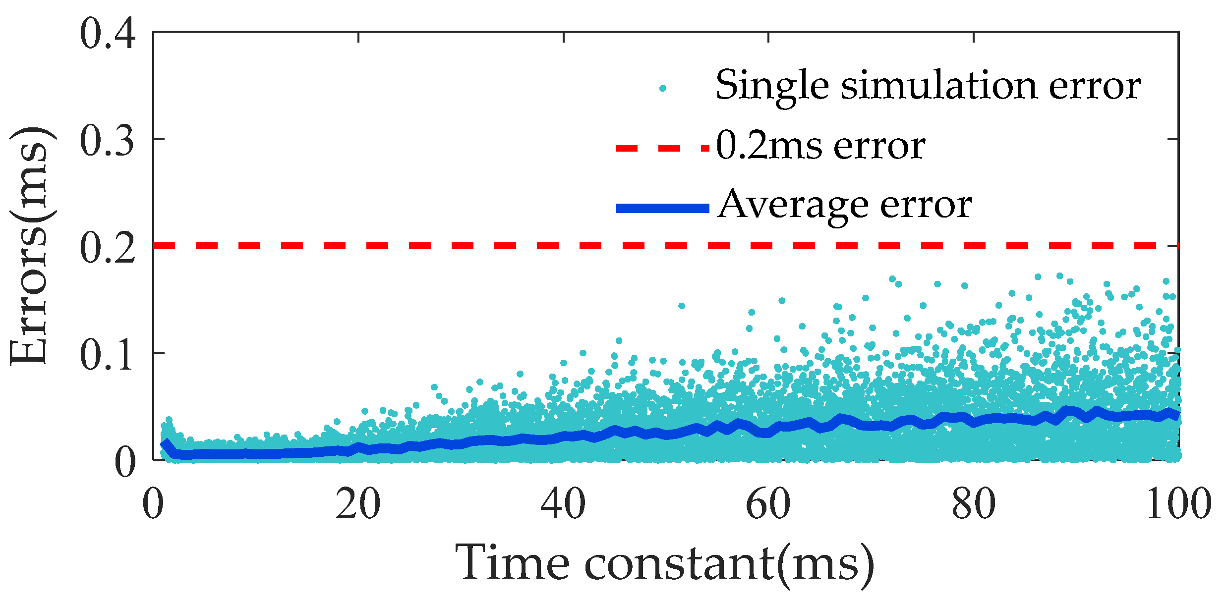
• The effect of the time constant on prediction error: The test shows that the prediction error increases gradually with the increase in time constant, but the error remains within 0.2 ms in the range of 100 ms.
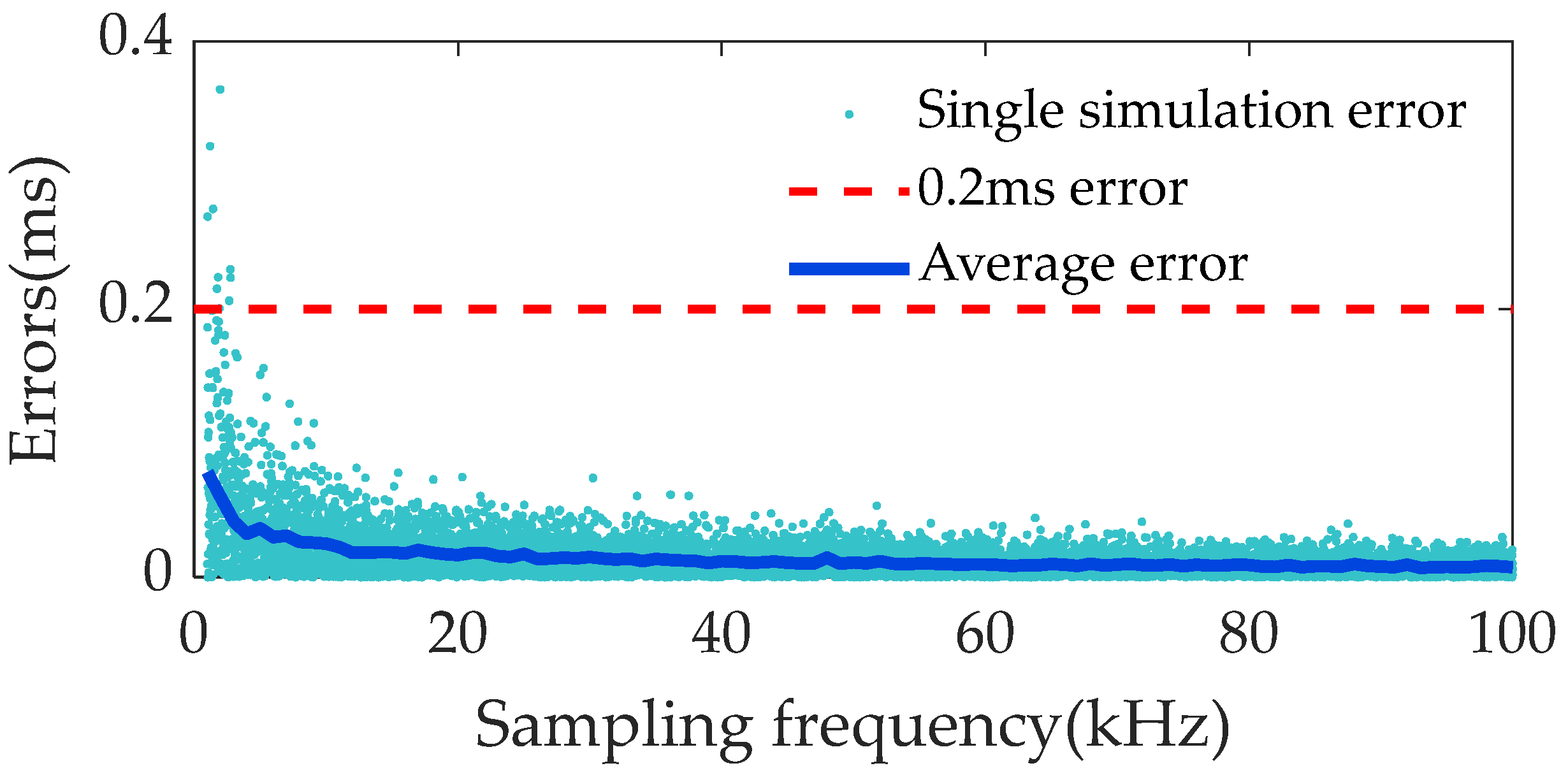
• Sampling frequency on prediction accuracy: Sampling frequency significantly affects the prediction accuracy. When the frequency is increased from 10 kHz to higher, the error is further reduced, and the improvement in accuracy tends to level off above 40 kHz, which verifies the positive effect of high frequency sampling on the accuracy of the algorithm.
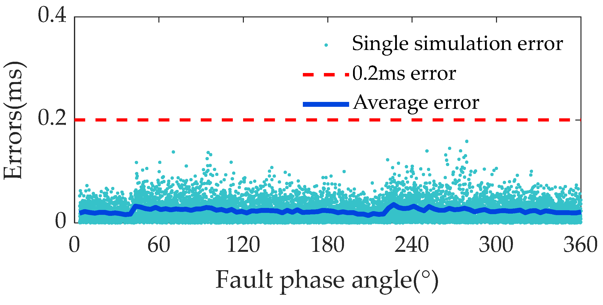
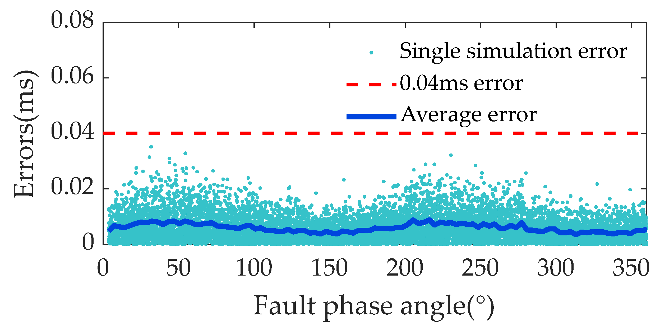
• Influence of fault phase angle: The test covers a range of fault phase angles from 1° to 360°, and the prediction errors fluctuate at specific phase angles; however, they are all within 0.2 ms, which indicates that the algorithm has a strong adaptability in dealing with different phase angles.
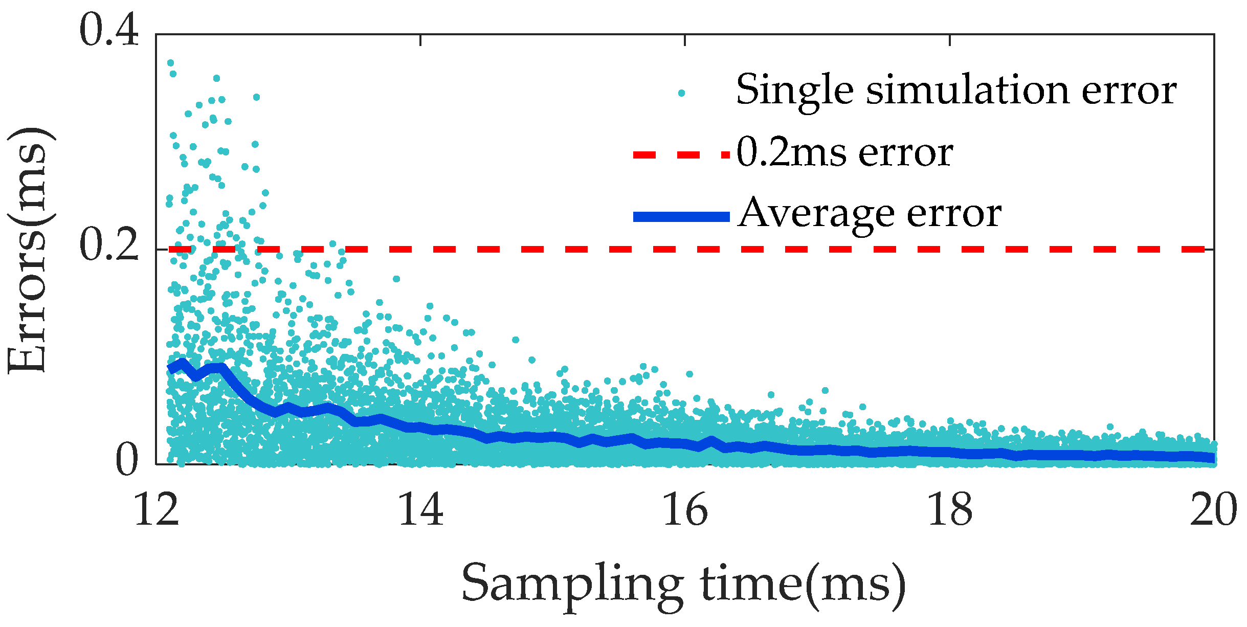
• Sampling time constraints: Too short a sampling time affects the algorithm’s accuracy, but when the sampling time exceeds 17 ms, the error stabilizes and is sufficient to meet the needs of engineering applications at 15 ms.

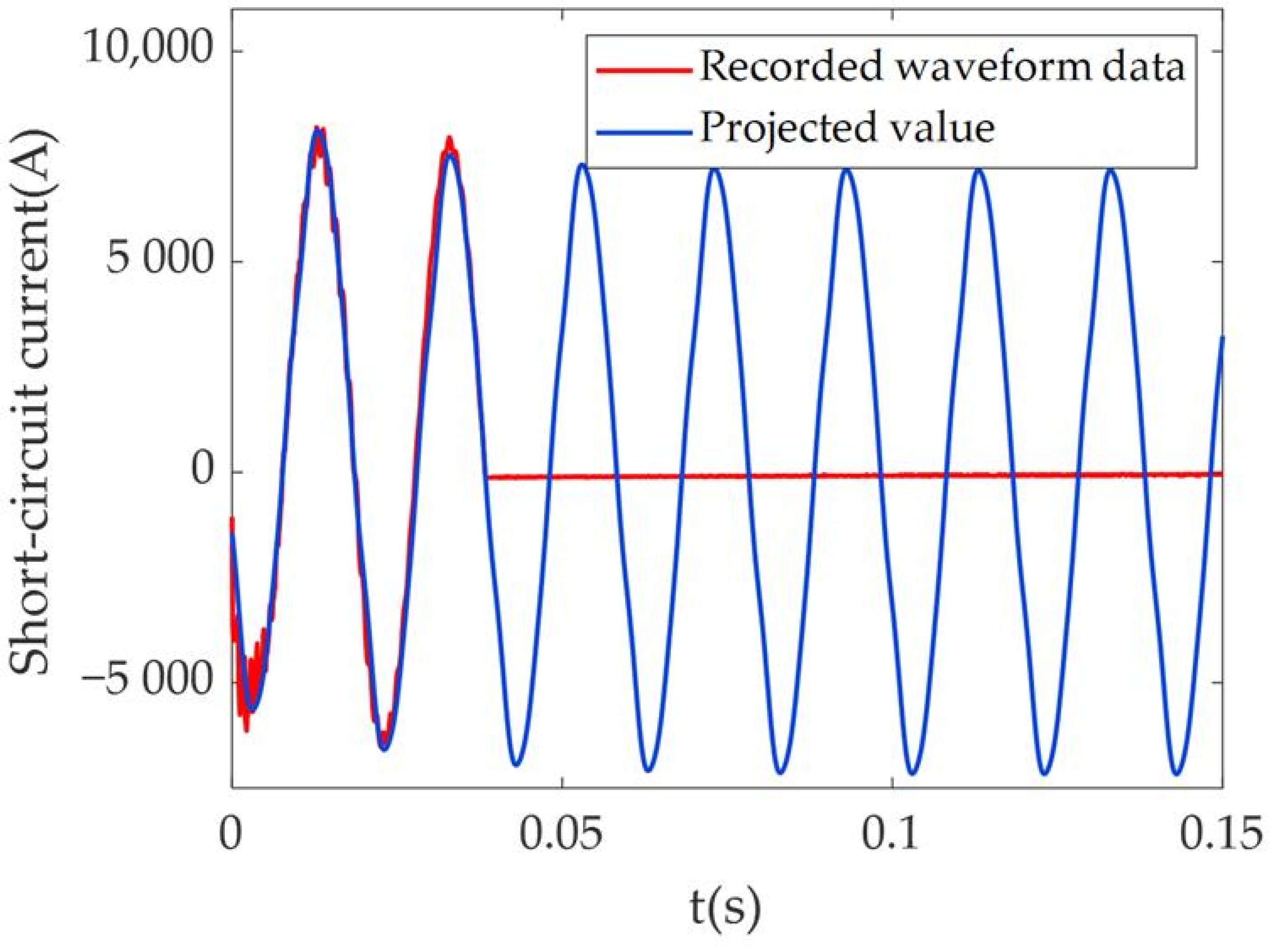
3.2. Validation of Recorded Waveform Data

The proposed algorithm was evaluated using recorded waveform data from a short-circuit fault incident in the China Southern Power Grid (CSG). Figure 7 demonstrates the prediction performance under 15 ms sampling conditions, where the predicted short-circuit current from the algorithm (blue solid line) shows strong agreement with the actual fault current (red solid line). The fault initiation occurred at t = 0 ms, with successful clearance achieved at 38.4 ms. Notably, the computational error for the fourth current zero-crossing point post-fault was measured at 0.077 ms. This precision satisfies the accuracy requirements specified in the CFI guidelines for zero-crossing point determination, particularly in critical power system protection applications.

4. Controlled Fault Current Interruption Sequence

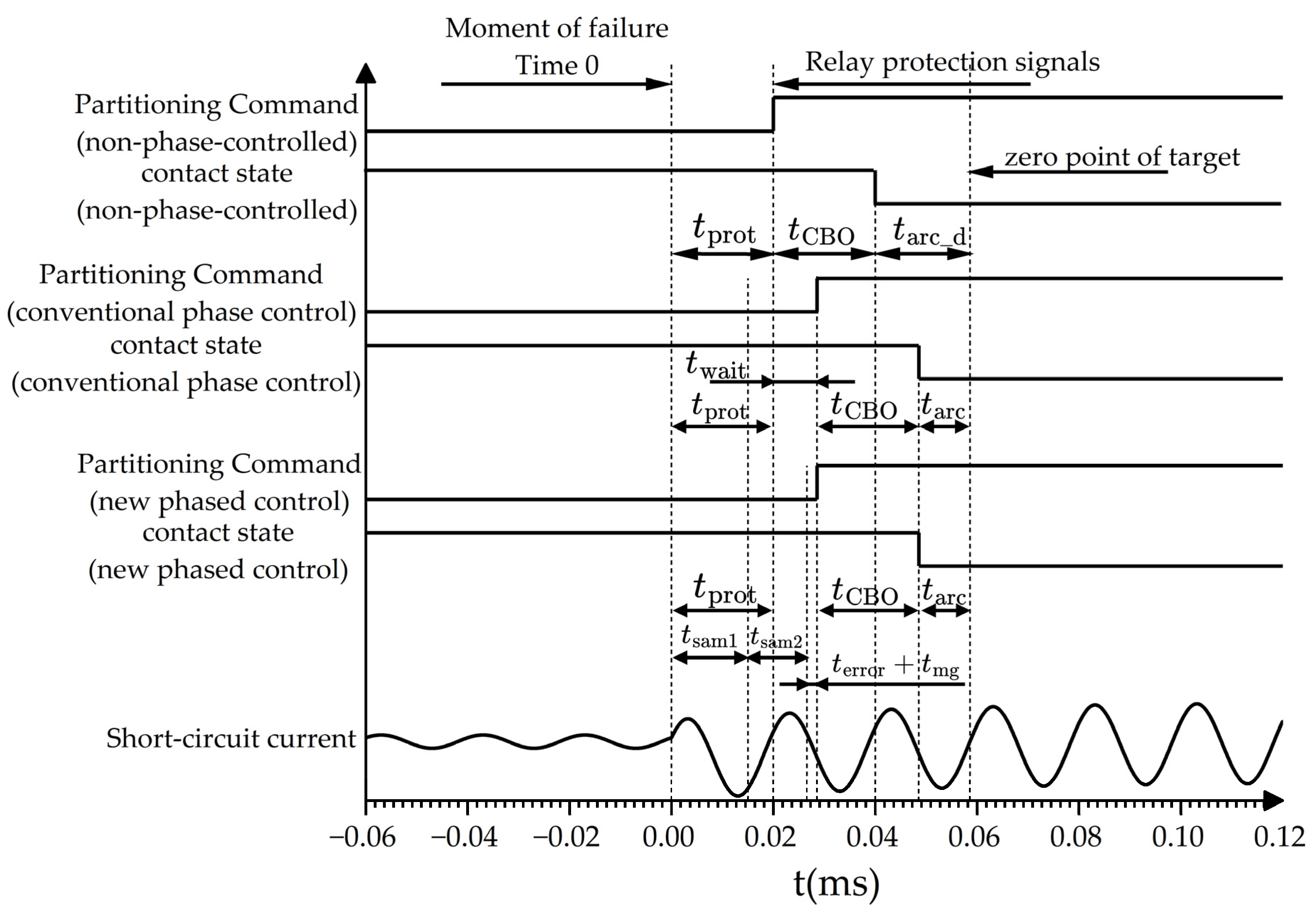
4.1. Double-Sample Time Interruption Sequence

In the case of non-phase-controlled interruption, the circuit breaker triggers the opening action after the relay protection time, the contacts begin to break after the breaker tripping time, and the arc is extinguished at current zero after the arcing time.

In conventional controlled fault current interruption sequences, after a fault occurs, the relay protection system is required to calculate the time coordinates of the target zero-crossing point within its response time [18]. Subsequently, the necessary waiting time is determined by combining the circuit breaker’s opening time and the minimum arc ignition time. However, this sequence can lead to a waiting time of up to about 10 ms, resulting in wasted sampling data during the waiting time.

In view of this, this study proposes a controlled fault current interruption sequence based on double-sampling. The sequence is based on the results of one calculation of the traditional sequence, using the waiting time with the remaining relay protection response time to continue optimizing the target zero calculation accuracy and reset the waiting time to complete the CFI. The specific steps are as follows:

• Set the first sampling time $t_{\mathrm{sam}1}$ within the response time of the relay protection, and use the data during this time to complete the calculation of the first target zero-crossing point $t_{\mathrm{zero}1}$.
• In order that the second calculation will not result in a negative waiting time, combine the results of the batch simulation to obtain the maximum error $t_{\mathrm{error}}$ of the first target zero-crossing point calculation, while considering the algorithm’s time margin $t_{\mathrm{mg}}$, to calculate the time interval $[t_{\mathrm{sample}1}{t}_{\mathrm{zero}1}-t_{\mathrm{mg}}-t_{\mathrm{error}}]$ of the supplementary data required for the second calculation.
• Based on the results of the first calculation, use the supplementary data to complete the second calculation before the calculation time threshold $t_{\mathrm{deadline}}=t_{\mathrm{zero}1}-t_{\mathrm{error}}$, to obtain the final confirmation of the target over-zero point $t_{\mathrm{zero}2}$. The upper limit of the time interval of the supplementary data to the second waiting time between the signals issued by the controlled switching device improves the accuracy of the calculation of the target over-zero point.
• If the first calculation fails, use the supplementary data to calculate the maximum error $t_{\mathrm{wait}2}$ of the first target over-zero point calculation.
• If the first calculation fails, issue a switching command at the end of the relay protection response time. If the second calculation fails, input $t_{\mathrm{zero}1}$ to the controlled switching device to realize controlled switching.

The sequence comparison of double-sampling time interruption with conventional controlled fault current interruption and non-phase-controlled interruption is shown in Figure 8.

The figure assumes that the target zero point calculated by the conventional controlled fault current interruption sequence and double-sampling time interruption sequence are error-free; then, the waiting time $t_{\mathrm{wait}2}$ after the completion of the second calculation in the double-sampling time CFI sequence is equal to the sum of $t_{\mathrm{error}}$ and $t_{\mathrm{mg}}$. Under the actual working condition, the double sampling time CFI sequence will calculate a more accurate zero coordinate $t_{\mathrm{zero}2}$ than the traditional sequence, and then wait time $t_{\mathrm{wait}2}=t_{\mathrm{zero}2}-(t_{\mathrm{sam}1}+t_{\mathrm{sam}2})$; after the upper limit of the supplementary data interval $t_{\mathrm{zero}1}-t_{\mathrm{mg}}-t_{\mathrm{error}}$, wait for $t_{\mathrm{wait}2}$ to issue a gate command to complete the controlled fault current interruption function.

4.2. Analysis of the Integrated Application of the Half-Cycle Elimination Method with Double-Sampling Time Interruption Sequences

In Section 2.2, the half-cycle elimination method introduced allows subsequent calculations to be updated based on the previous results by employing the recursive least squares method. This method, in combination with the double-sampling-based fault current interruption sequence, is able to fully utilize the waiting time and the remaining relay protection response time to further enhance the calculation accuracy of the non-periodic component parameters through RLS. The computational flow of the combination of the two is shown in Figure 9.

The waiting time is mainly caused by the mismatch between the target phase and the sequence of the breaking time and the arc burning time, etc. Therefore, the performance of the combination of the half-cycle elimination method and the double-sampling time CFI sequence should be evaluated for different fault phase angles when testing the performance of the half-cycle elimination method and the double-sampling time CFI sequence. The test is conducted using the same parameter settings as reported in Section 2.1, and the results are shown in Figure 10.

The results show that the half-cycle elimination method combined with the controlled fault current interruption sequence with double-sampling time improves the accuracy of the calculation of the target AC zero by an order of magnitude compared to the method combined with the conventional controlled fault current interruption sequence.

Table 2. Sampling time and error comparison of different zero prediction algorithms.

Method Name	Sampling Time	Inaccuracies
Adaptive RLS Algorithm [18]	15 ms	0.4 ms
Improved Half-wave Fourier Algorithm [23]	10 ms + 2 sampling points	1 ms
WLMS Algorithm [24]	10 ms	1 ms
Half-cycle elimination method	15 ms	0.2 ms
Half-cycle elimination method with double-sampling sequence	15 ms	0.04 ms

shows the sampling time required by several different zero prediction algorithms and their corresponding zero prediction errors, from which it can be seen that the half-cycle elimination method has a higher prediction accuracy. In addition, the half-cycle elimination method with double-sampling sequence can achieve a huge improvement in prediction accuracy without increasing the sampling time.

5. Conclusions

• A half-period elimination method is innovatively proposed in this paper to accurately predict the zero-crossing point of short-circuit currents. The periodic and non-periodic components are separated, and the recursive least squares method combined with fast Fourier transform is applied to enable the real-time and precise prediction of short-circuit currents.
• Simulation and recording tests are carried out for the half-period elimination method, and the results show that the prediction error of the sixth zero-crossing point of the algorithm is less than 0.2 ms under the conditions of adding 40 dB noise, a sampling frequency of more than 10 kHz, and a sampling time of more than 15 ms, which is of practical value.
• In order to solve the time-wasting problem that may occur in the traditional controlled fault current interruption sequence, this paper further develops a double-sampling controlled fault current interruption sequence. The sequence optimizes the calculation process of the target over-zero point and improves the accuracy and timeliness of prediction through two-stage sampling and calculation. Experimental results show that the sequence can significantly improve the accuracy of over-zero point prediction and effectively reduce the waiting time of the system.

References

1. Kasikci, I. Short Circuits in Power Systems: A Practical Guide to IEC 60909-0; John Wiley & Sons: Hoboken, NJ, USA, 2018. [Google Scholar]
2. Tleis, N.D. Power Systems Modelling and Fault Analysis: Theory and Practice; Newnes: New South Wales, Australia, 2008. [Google Scholar]
3. Yadav, S.; Suman, G.K.; Mehta, R.K. Study of electromagnetic forces on windings of high voltage transformer during short circuit fault. In Proceedings of the 2020 3rd International Conference on Energy, Power and Environment: Towards Clean Energy Technologies, Sydney, Australia, 20–22 April 2021; pp. 1–5. [Google Scholar]
4. Kothavade, J.U.; Kundu, P. Investigation of electromagnetic forces in converter transformer. In Proceedings of the 2021 IEEE 2nd International Conference on Smart Technologies for Power, Energy and Control (STPEC), Noida, India, 29–31 July 2021; pp. 1–6. [Google Scholar]
5. Kodama, Y.; Otani, K. Short-Circuit Point Estimation Method for Distribution Lines Using Smart-Meters. IEEJ Trans. Electr. Electron. Eng. 2024, 19, 1976–1986. [Google Scholar] [CrossRef]
6. Zhang, Y.; Pei, X.; Li, Z.; Zhou, P. Short-circuit current limiting control strategy for single-phase inverter based on adaptive reference feedforward and third harmonic elimination. IEEE Trans. Power Electron. 2021, 37, 5320–5332. [Google Scholar] [CrossRef]
7. Zhang, T.; Zhou, Q.; Bian, X. Research on Electromagnetic Characteristics of Interturn Short Circuit in Three Phase Transformers. In Proceedings of the 2024 3rd International Conference on Energy, Power and Electrical Technology (ICEPET), Beijing, China, 26–28 April 2024; pp. 1039–1043. [Google Scholar]
8. Glover, J.D.; Overbye, T.J.; Sarma, M.S. Power System Analysis & Design; Cengage Learning: Boston, MA, USA, 2017. [Google Scholar]
9. Jyothi, M.N.; Upadhayay, P.; Reddy, M.D.K.; Rishitha, N. Comparison of Restricted Earth Fault Current Devices for Various Earthing Systems Using ETAP Software. In Proceedings of the 2024 10th International Conference on Advanced Computing and Communication Systems (ICACCS), Coimbatore, India, 19–21 January 2024; pp. 535–540. [Google Scholar]
10. Xingjian, W.; Jing, S.; Hongkun, C. Short Fault Current Zero Point Drift and Phase-Controlled Interruption Strategy in Three-Phase Power Transmission Lines. In Proceedings of the Annual Conference of China Electrotechnical Society, Chengdu, China, 8–10 December 2023; pp. 46–55. [Google Scholar]
11. Li, L.; Wang, D.; Yang, H.; Xiang, B.; Ma, F.; Yu, J.; Li, Y.; Liu, Z. Short-Circuit Fault Current Phase-Controlled Switching Method Based on Fast Vacuum Circuit Breaker. In Proceedings of the 2024 7th International Conference on Electric Power Equipment-Switching Technology (ICEPE-ST), Shenzhen, China, 19–21 April 2024; pp. 228–231. [Google Scholar]
12. Wen, H.; Zhang, J.; Yao, W.; Tang, L. FFT-based amplitude estimation of power distribution systems signal distorted by harmonics and noise. IEEE Trans. Ind. Inform. 2017, 14, 1447–1455. [Google Scholar] [CrossRef]
13. Peng, H.; Zhu, L.; Mo, W.; Wang, Y.; He, Q.; Wu, X. Zero-crossing Prediction of Short-circuit Current Using Recursive Least Square Algorithm. In Proceedings of the 2020 5th Asia Conference on Power and Electrical Engineering (ACPEE), Bangkok, Thailand, 16–18 March 2020; pp. 1360–1364. [Google Scholar]
14. Chen, Q.; Zhang, G.; Liu, J.; Geng, Y.; Wang, J. Study on fast early detecting and rapid accurate fault parameters estimation method for short-circuit fault. In Proceedings of the 2017 4th International Conference on Electric Power Equipment-Switching Technology (ICEPE-ST), Shenzhen, China, 3–5 November 2017; pp. 509–513. [Google Scholar]
15. Cao, J.; Zhao, Y.; Zhang, N.; Wang, W.; Wang, D. A research on zero-cross point forecast method of short circuit current. In Proceedings of the 2017 IEEE 2nd Advanced Information Technology, Electronic and Automation Control Conference (IAEAC), Chengdu, China, 24-26 November 2017; pp. 2385–2389. [Google Scholar]
16. Poltl, A.; Frohlich, K. A new algorithm enabling controlled short circuit interruption. IEEE Trans. Power Deliv. 2003, 18, 802–808. [Google Scholar] [CrossRef]
17. Huang, L.; Zhang, L.; Hu, Y.; Yang, H.; Xiang, B.; Yao, X. Fast prediction method of short-circuit current zero based on an algorithm of long short term memory [J/OL]. High Volt. Eng. 2023, 12, 1–10. [Google Scholar] [CrossRef]
18. Huang, Z.; Zhang, D.; Zou, J.; Dong, W. Design of control system for controlled fault interruption based on adaptive RLS algorithm. High Volt. Eng. 2016, 42, 3214–3220. [Google Scholar] [CrossRef]
19. Xiongying, D.; Zhihui, H.; Rui, L. Comparison between two methods of zero-cross point prediction for controlled fault current interruption. High Volt. Electr. Appl. 2011, 47, 5–9. [Google Scholar] [CrossRef]
20. de Metz-Noblat, B.; Dumas, F.; Poulain, C. Calculation of short-circuit currents. Cah. Tech. 2005, 158, 1–32. [Google Scholar]
21. Benesty, J.; Paleologu, C.; Gänsler, T.; Ciochină, S.; Benesty, J.; Paleologu, C.; Gänsler, T.; Ciochină, S. Recursive least-squares algorithms. In A Perspective on Stereophonic Acoustic Echo Cancellation; Springer: Berlin/Heidelberg, Germany, 2011; pp. 63–69. [Google Scholar] [CrossRef]
22. Bai, Y.; Li, S.; Chen, W.; Wu, T.; Zhou, L. Study on the time constant of DC component and its influence on short-circuit breaking capacity of circuit breaker. In Proceedings of the 2018 IEEE 4th Information Technology and Mechatronics Engineering Conference (ITOEC), Chengdu, China, 14–16 December 2018; pp. 1929–1932. [Google Scholar]
23. Luo, C.-j.; Yuan, Z.; Yin, X.-G.; He, J.-J.; Chen, X.-S.; Pan, Y. Zero-cross point prediction of short circuit current for phase controlled interruption based on improved half-wave Fourier algorithm. High Volt. Appar. 2012, 48, 1–6. [Google Scholar] [CrossRef]
24. Fang, C.; Lin, M.; Li, W. Investigation on controlled fault current interruption of high voltage circuit breaker based on WLMS algorithm. High Volt. Appar. 2009, 45, 40–43. [Google Scholar] [CrossRef]
Figure 1. Single-phase short-circuit model.
Applsci 15 03106 g001
Figure 2. Schematic diagram of prediction failure.
Applsci 15 03106 g002
Figure 3. Zero prediction error versus time constant.
Applsci 15 03106 g003
Figure 4. Zero prediction error versus sampling frequency.
Applsci 15 03106 g004
Figure 5. Zero point prediction error versus fault phase angle.
Applsci 15 03106 g005
Figure 6. Zero prediction error versus sampling time.
Applsci 15 03106 g006
Figure 7. Recovered waveform of fault recording data.
Applsci 15 03106 g007
Figure 8. Comparison of the CFI on–off sequence with dual sampling time.
Applsci 15 03106 g008
Figure 9. Flowchart of half-cycle elimination method with double-sampling time interrupt sequence.
Applsci 15 03106 g009
Figure 10. Effect of half-cycle elimination method with double-sampling sequence calculation.
Applsci 15 03106 g010