A Temporal Convolutional Network–Bidirectional Long Short-Term Memory (TCN-BiLSTM) Prediction Model for Temporal Faults in Industrial Equipment

Abstract

Traditional algorithms and single predictive models often face challenges such as limited prediction accuracy and insufficient modeling capabilities for complex time-series data in fault prediction tasks. To address these issues, this paper proposes a combined prediction model based on an improved temporal convolutional network (TCN) and bidirectional long short-term memory (BiLSTM), referred to as the TCN-BiLSTM model. This model aims to enhance the reliability and accuracy of time-series fault prediction. It is designed to handle continuous processes but can also be applied to batch and hybrid processes due to its flexible architecture. First, preprocessed industrial operation data are fed into the model, and hyperparameter optimization is conducted using the Optuna framework to improve training efficiency and generalization capability. Then, the model employs an improved TCN layer and a BiLSTM layer for feature extraction and learning. The TCN layer incorporates batch normalization, an optimized activation function (Leaky ReLU), and a dropout mechanism to enhance its ability to capture multi-scale temporal features. The BiLSTM layer further leverages its bidirectional learning mechanism to model the long-term dependencies in the data, enabling effective predictions of complex fault patterns. Finally, the model outputs the prediction results after iterative optimization. To evaluate the performance of the proposed model, simulation experiments were conducted to compare the TCN-BiLSTM model with mainstream prediction methods such as CNN, RNN, BiLSTM, and A-BiLSTM. The experimental results indicate that the TCN-BiLSTM model outperforms the comparison models in terms of prediction accuracy during both the modeling and forecasting stages, providing a feasible solution for time-series fault prediction.

1. Introduction

With the rapid development of industrialization and intelligent technologies, modern industrial equipment and mechanical systems are increasingly evolving towards greater complexity, precision, and integration. These systems are widely applied in fields such as manufacturing, transportation, energy production, and intelligent logistics, playing an indispensable role in ensuring the efficient operation of the national economy and social activities [1]. However, as system complexity and operational loads continue to increase, the probability of faults and their unpredictability also rise. This not only poses significant challenges to the safe operation of equipment but may also lead to substantial economic losses and safety risks [2].

Unexpected failures of industrial equipment are phenomena that are difficult to completely avoid, and their impacts often go beyond production downtime, potentially causing cascading system damage. For instance, in the field of energy production, issues such as turbine blade wear, cracks, or excessive vibrations can significantly reduce power generation efficiency and even lead to catastrophic shutdown accidents. In the transportation sector, abnormal temperature rises or fatigue cracks in train bearings may become critical triggers for operational failures, thereby endangering passenger safety [3]. Consequently, ensuring the safe and efficient operation of mechanical systems has become a core requirement for modern industrial development. To achieve this, the timely prediction of potential equipment failures and the implementation of preventive maintenance measures have become critical technological approaches to mitigate operational risks and control maintenance costs [4].

The core of fault prediction technology lies in real-time monitoring of the operating states of industrial equipment to establish a mapping relationship between equipment characteristics and health conditions. This enables the prediction of potential fault modes and the estimation of fault occurrence times. In recent years, this field has garnered significant attention from both industry and academia, achieving rapid advancements in areas such as intelligent manufacturing, the Industrial Internet of Things (IIoT), and Prognostics and Health Management (PHM). However, traditional fault diagnosis methods—such as rule-based periodic maintenance or diagnostic analysis relying on human expertise—often exhibit considerable limitations when dealing with complex and diverse industrial equipment. These limitations arise mainly due to the following distinctive challenges associated with modern industrial equipment:

• High Complexity: Industrial equipment typically consists of multiple highly coupled subsystems, with operating states characterized by strong nonlinearity and dynamic coupling. This makes it challenging to accurately describe the overall system behavior using simple physical models.
• High Dynamism: Industrial equipment operates in complex and ever-changing environments, and its operating parameters (e.g., vibration, temperature, and current) fluctuate significantly over time. Traditional static analysis methods struggle to capture these dynamic variations effectively.
• Fault Concealment: Certain potential faults (e.g., early-stage cracks and minor wear) have minimal impact on the operational state in their initial stages, making them difficult to detect through conventional monitoring techniques.

To address the aforementioned challenges, machine learning and deep learning technologies offer novel research avenues for fault prediction in complex equipment. These techniques can automatically extract critical features from massive sensor data and construct nonlinear, multi-layered fault prediction models. Monitoring data from industrial equipment are typically presented as time-series data, encompassing various physical quantities collected by multiple sensors, such as vibration signals, current, voltage, and temperature. These data are characterized by high dimensionality, nonlinearity, and noise interference, making it difficult for traditional methods to model them comprehensively. The complexity of equipment structures and operating conditions results in fault patterns with multiple mechanisms (e.g., mechanical wear, fatigue, overloading, and nonlinear vibrations) and interactions between fault modes, complicating their analysis and prediction. In practical industrial scenarios, fault data are typically scarce and unevenly distributed. Healthy state data dominate the datasets, while fault state data are often limited and insufficient. This imbalance poses challenges for training models that can effectively recognize and predict faults.

Current research methods for time-series fault prediction can be broadly divided into two categories: statistical model-based methods and artificial intelligence (AI)-based methods.

• Statistical Model-Based Methods. These methods use linear or nonlinear regression models to analyze the relationships between equipment operating parameters and potential faults, building predictive models based on historical data. One of the main advantages of these methods is their simplicity, ease of implementation, and, importantly, their transparency and interpretability. This makes them not only easier to implement but also more likely to be accepted as effective prediction tools. However, their performance can be limited when handling large datasets with complex relationships [5]. For example, traditional time-series statistical models can effectively capture the temporal dependencies of faults. However, they generally assume linearity in the data, which limits their ability to address nonlinear issues [6,7].
• AI-Based Methods. Machine learning methods can extract features from large historical datasets, enabling the recognition of complex, nonlinear fault patterns and improving prediction accuracy. However, these approaches often require extensive manual feature selection and extraction, which can be time-consuming and labor-intensive [8]. Expert systems, on the other hand, can make quick predictions and decisions for specific fault patterns, but they rely heavily on domain experts’ knowledge and experience, which limits their scalability and generalizability [9]. Long short-term memory (LSTM) networks, specifically designed to handle sequential data, have demonstrated strong capabilities in capturing long-term dependencies in time-series data. By leveraging mechanisms for memory retention and forgetting, LSTMs dynamically adjust the focus on prior information, resulting in more accurate fault predictions [10,11,12]. However, LSTM models are sensitive to noise, and their learning capacity may be adversely affected when processing data with significant noise levels. Given the inherent limitations of both statistical model-based and AI-based approaches, hybrid predictive models have emerged as a promising solution. These models combine the strengths of different methods, offering more accurate and stable prediction performance compared to standalone models [13].

To enhance the accuracy and stability of industrial equipment fault prediction, this paper proposes a hybrid predictive model based on the temporal convolutional network (TCN) and bidirectional long short-term memory network (BiLSTM). The main contributions of this study are summarized as follows:

• A novel TCN-BiLSTM hybrid model is proposed, which integrates the ability of BiLSTM to capture bidirectional dependencies in time-series data with the efficient multi-scale temporal feature extraction capability of TCN. This combination improves the model’s ability to process complex time-series data.
• The proposed model incorporates techniques such as batch normalization, dropout, and an optimized Leaky ReLU activation function into the network structure. These enhancements effectively mitigate the vanishing and exploding gradient problems in deep networks, significantly improving the training efficiency and stability of the model.
• The model leverages the Optuna framework for hyperparameter optimization, enabling the selection of optimal parameters tailored to different datasets. This approach enhances the model’s generalization capability across diverse applications.

In addition to the performance during the modeling phase, the predictive phase is equally critical for evaluating the practical value of fault prediction algorithms. During the predictive phase, models often encounter previously unseen data distributions, while observation data in industrial scenarios are frequently accompanied by noise, uncertainty, and unknown error structures. Therefore, a successful predictive model must not only exhibit strong modeling capabilities but also effectively handle noise interference and observational errors during the predictive phase to ensure the robustness and reliability of its predictions.

The proposed TCN-BiLSTM model leverages multi-scale temporal feature extraction and bidirectional sequential dependency modeling, giving it the theoretical and practical ability to address complex observational errors. Furthermore, the network design incorporates techniques such as batch normalization, Leaky ReLU activation functions, and residual connections. These mechanisms significantly mitigate the impact of noise during the predictive phase and enhance the model’s adaptability to unseen data distributions.

2. TCN-BiLSTM Predictive Model

2.1. TCN Model Architecture

TCN is a temporal convolutional network specifically designed for time-series data processing. Compared to traditional Convolutional Neural Networks (CNNs), TCN introduces causal convolutions to ensure that the output at any given time step does not depend on future time steps, preserving the temporal order of the data. Furthermore, through the use of dilated convolutions, TCN can effectively expand its receptive field without increasing the number of parameters, allowing it to capture long-range dependencies within sequences. The basic structure of the dilated convolutions model is illustrated in Figure 1. The receptive field regions of the TCN with different dilation factors (d = 4, d = 2, and d = 1) are also depicted.

The calculation formulas for the causal convolution in TCN are shown as follows:

$$y(t)={\displaystyle \sum _{k=0}^{K-1}f(k)\cdot x(t-d\cdot k)}$$

(1)

In this equation, x(t) denotes the input sequence, f represents the convolutional kernel, K is the kernel size, y(t) is the output sequence, and d is the dilation rate.

To mitigate the overfitting issue in the network and enhance its performance, learning efficiency, and accuracy, techniques such as batch normalization, activation functions, and dropout are commonly used. Additionally, to ensure connection stability in deep TCN networks, residual connections are introduced. Combined with other methods, these form the residual module, which further optimizes the performance of TCN.

In this study, Leaky ReLU is employed as the activation function instead of the traditional ReLU. Leaky ReLU retains a small slope on the negative axis, allowing some negative values to pass through. This prevents the issue of completely inactive neurons for negative inputs, which is commonly observed with ReLU. Leaky ReLU is more adaptive to time-series data with uneven feature distributions. The formula is expressed as follows:

$$f(x)=\left\{\begin{array}{l}x,x>0\\ ax,x\le 0\end{array}\right.$$

(2)

In this formula, x represents the input value, and “a” denotes the slope for the negative input region. The ax part indicates that when the input x is negative, the output will be the product of the input value x and the constant “a”. Here, “a” is a small constant, typically set to 0.01, which ensures that there is still a slight output even for negative inputs. This prevents neurons from becoming “dead”—that is, not activating at all—when faced with negative input.

2.2. BiLSTM Model Architecture

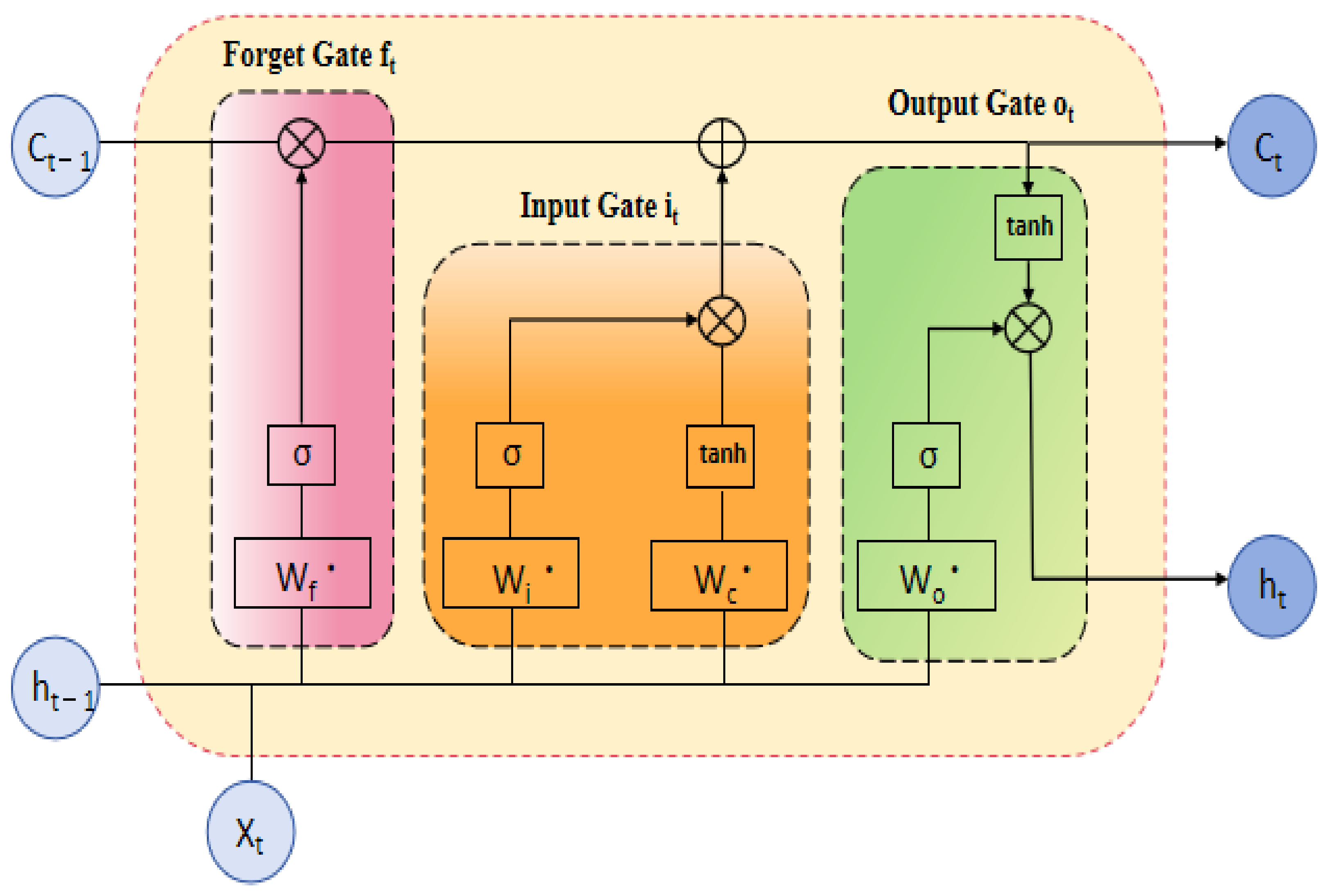
LSTM (long short-term memory) is a specialized type of recurrent neural network (RNN) designed for processing and predicting sequential data. Its core lies in the gating mechanism, which regulates the flow of information through the forget gate, input gate, and output gate [14]. These gates work together to manage the storage of short-term and long-term memory via the hidden state and cell state. By addressing the vanishing gradient problem inherent in standard RNNs [15], LSTMs are particularly effective in learning from long sequences. The specific structure of a single-layer LSTM cell is illustrated in Figure 2 [16].

In LSTM, the sigmoid function plays a crucial role in regulating the flow of information by mapping input values to a range of (0, 1). This enables the normalization of outputs for each neuron and helps determine the extent to which different pieces of information are stored or forgotten within the network. Due to these characteristics, the sigmoid function is well suited as the activation function in the gating mechanism.

$$\sigma (x)={\displaystyle \frac{1}{1+e^{-x}}}$$

(3)

In this equation, σ represents the sigmoid activation function.

The hidden state reflects the “memory” of sequential data at the current time step. By being updated iteratively, it dynamically extracts and retains features relevant to the current prediction task.

$$h_t^l=o_t^l\cdot \tanh (C_t^l)$$

(4)

In the equation, l represents the number of LSTM layers, C_t represents the cell state, and tanh represents the hyperbolic tangent activation function, which ensures that the generated hidden state is constrained within the range of [−1, 1].

The forget gate often functions to regulate the proportion of past information retained, determining the extent to which information from the cell state C_t−1 at the previous time step is preserved.

$$f_t^l=\sigma (W_f^l\cdot [h_{t-1}^l,x_t]+b_f^l)$$

(5)

In the equation, W_f represents the weight matrix of the forget gate, and b_f represents the bias matrix of the forget gate.

The input gate is responsible for determining the information to be updated in the cell state.

$$i_t^l=\sigma (W_i^l\cdot [h_{t-1}^l,x_t]+b_i^l)$$

(6)

In this equation, W_i represents the weight matrix of the input gate, and b_i represents the bias matrix of the input gate.

Meanwhile, at each time step, the candidate cell state is computed based on the current input vector x_t and the hidden state h_t−1 from the previous time step.

$${\tilde{C}}_t^l=\tanh (W_c^l\cdot [h_{t-1}^l,x_t]+b_c^l)$$

(7)

In this equation, W_c represents the weight matrix of the cell state, and b_c represents the bias matrix of the cell state.

The cell state is updated through the operations of the forget gate and the input gate.

$$C_t^l=f_t^l\cdot C_{t-1}^l+i_t^l\cdot {\tilde{C}}_t^l$$

(8)

Finally, the output gate is computed.

$$o_t^l=\sigma (W_o^l\cdot [h_{t-1}^l,x_t]+b_o^l)$$

(9)

In this equation, W_o represents the weight matrix of the output gate, and b_o represents the bias matrix of the output gate.

In fault prediction, early signs of certain faults may emerge at later time steps, which standard LSTM models may fail to capture. If LSTM considers both forward and backward information at each time step, it can significantly enhance the model’s ability to capture contextual information and improve the accuracy of equipment fault prediction. Moreover, considering that fault manifestations may become more complex in certain scenarios, stacking multiple layers of bidirectional LSTM allows each layer to learn features at different levels, enabling deeper feature extraction.

This paper proposes a deep bidirectional long short-term memory network model. On the basis of standard LSTM, the model incorporates a backward LSTM and employs a stacked structure. The architecture of the proposed model is shown in Figure 3.

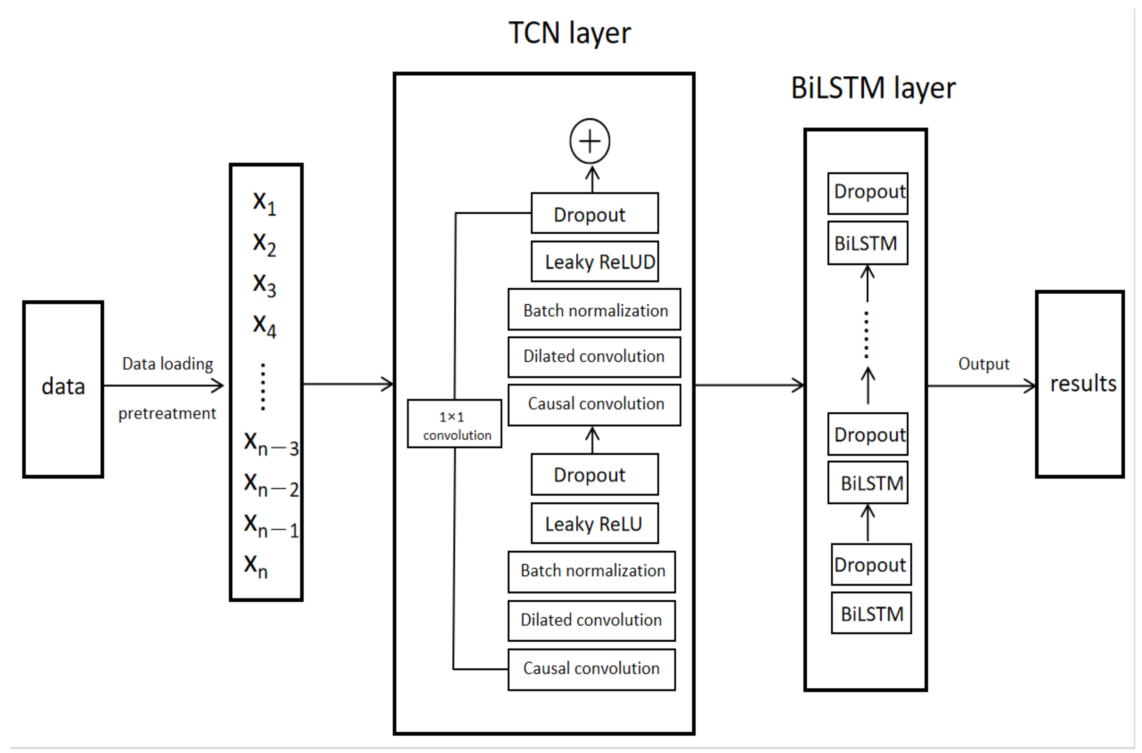
2.3. TCN-BiLSTM Prediction Method

The structure of the TCN-BiLSTM model is mainly divided into three components: the data preprocessing module, the TCN layer, and the BiLSTM layer. The detailed architecture of the model is illustrated in Figure 4.

In practical industrial applications, the predictive phase of a model often encounters challenges such as unmodeled noise, observational errors, and uneven data distributions in industrial sensor data. The proposed model, through its design and mechanisms, not only enhances its capability during the modeling phase but also improves its robustness during the predictive phase.

The TCN layer serves as the first core component of the model, specifically designed for feature extraction from time-series data. To enhance the model’s performance, the TCN layer adopts the following technical designs:

• Causal Convolution: Causal convolution in TCN is one of its core features, ensuring that the output at each time step only depends on the current and past time steps. This means that future time steps (potential sources of noise) do not influence the prediction of the current time step, thereby preventing future information from interfering with the model’s training and reducing the risk of noise propagating to subsequent time steps.
• Dilated Convolution: Dilated convolution increases the receptive field of the convolution, enabling the model to capture longer temporal dependencies without adding more parameters. Dilated convolution helps reduce the impact of noise on short time scales, thereby allowing the model to more stably capture key dynamic changes in long time series. When dealing with industrial time-series data, noise typically manifests as high-frequency signals. Dilated convolution effectively diminishes the interference of high-frequency noise, allowing the model to focus more on the long-term trends of the sequence rather than on local random fluctuations.
• Leaky ReLU Activation Function: Compared to the traditional ReLU activation function, the Leaky ReLU activation function maintains a small slope for negative inputs, effectively preventing the “dying neuron” problem. Noisy data often contain negative values, and Leaky ReLU can effectively mitigate the impact of noise on the network, allowing the neural network to continue training effectively even in the presence of noise. This enhances the model’s robustness and its ability to capture nonlinear features.
• Dropout: By randomly dropping out a portion of neurons during training, dropout effectively combats overfitting and enhances the model’s generalization capabilities. This technique “turns off” a random subset of neurons during each iteration, reducing dependencies between neurons and improving the model’s ability to adapt to unseen data. Dropout is a simple yet powerful regularization method commonly used in deep neural networks, particularly in deeper architectures, to significantly boost performance.
• Batch Normalization: Batch normalization normalizes the inputs to each layer by adjusting their mean to 0 and variance to 1, thus mitigating the internal covariate shift and improving model stability. This technique accelerates convergence during training, alleviates the vanishing gradient problem, and enhances the stability of the training process. Additionally, batch normalization can act as a form of regularization, reducing the risk of overfitting.

Additionally, to facilitate efficient information flow and alleviate the gradient vanishing problem in deep networks, the TCN layer incorporates a 1×1 convolutional residual connection mechanism, ensuring smooth feature propagation between the input and output.

Building on the deep features extracted by the TCN layer, the BiLSTM layer further models the time-series data. Compared to traditional LSTM, BiLSTM captures bidirectional dependencies in the time series, providing a more comprehensive understanding of the dynamic characteristics of fault data. Since minority class faults typically have fewer samples and may occur at specific time points, BiLSTM can capture these critical pieces of information through its bidirectional structure, thereby enhancing the detection capability for minority class faults. By stacking multiple layers, the BiLSTM enhances its capacity to learn complex fault patterns. Moreover, for different application scenarios, the model leverages hyperparameter optimization (based on the Optuna framework) to fine-tune critical parameters such as the number of hidden units, learning rate, and regularization, effectively improving the model’s robustness and adaptability.

Both the TCN and BiLSTM layers in this model are designed as multi-layer structures. By conducting hyperparameter optimization tailored to specific problems, the model not only utilizes the TCN layer to capture multi-scale temporal features but also employs the BiLSTM layer to further extract long-term dependencies from the data. This complementary deep learning framework integrates features across different levels, significantly enhancing the model’s generalization and overall adaptability.

3. Simulation Experiments

3.1. Simulation Data

To validate the effectiveness and superiority of the proposed hybrid model, simulation experiments were conducted to evaluate its performance. The experiments were implemented based on the TensorFlow deep learning framework. The detailed experimental environment configuration is presented in

Table 1. Experimental environment configuration.

Environment	Specifications
Operating System	Windows11 (Version 22H2)
CPU	13th Gen Intel(R) Core(TM) i9-13900HX 2.20 GHz
GPU	NVIDIA GeForce RTX 4080
Memory	32 GB
Software	Visual Studio 2022 (Version 17.5.4)
Language	Python 3.9.12
CUDA	11.7.1

.

The AI4I 2020 Predictive Maintenance Dataset was used as the test dataset for this experiment. This dataset reflects real-world predictive maintenance scenarios, consisting of a total of 100,000 samples, 8 features, and 6 labels. The 8 features include UID, product ID, air temperature, process temperature, rotational speed, torque, and tool wear. The 6 labels represent different types of failures, which include overall failure, tool wear failure, heat dissipation failure, power failure, overstrain failure, and random failure.

Specific details of the fault types are summarized in

Table 2. Fault descriptions.

Fault Label	Description
Machine Failure	This indicates whether the equipment has experienced any failure.
Tool Wear Failure	Failure occurs when the equipment reaches the end of its tool wear lifespan or requires replacement.
Heat Dissipation Failure	Failure is caused by inadequate heat dissipation due to the equipment’s condition and temperature.
Power Failure	Failure occurs when the equipment’s power exceeds the power supply threshold.
Overstrain Failure	Failure is caused by excessive mechanical strain on the equipment.
Random Failure	Failure occurs due to random, unpredictable factors.

.

To validate the effectiveness of the proposed model, the dataset was divided into a training set and a testing set in a ratio of 80% to 20%. Specifically, 80,000 samples were randomly selected for model training, while the remaining 20,000 samples were used to evaluate the model’s performance. The datasets used for training and testing are contiguous in the time domain. This partitioning strategy ensures that the training data are sufficient for the model to learn effectively, while also leaving enough samples in the testing set to comprehensively assess the model’s generalization ability.

During the training phase, the training set was used to optimize the model’s parameters, ensuring that the model learns the mapping relationship between input features and output labels. The testing set, on the other hand, was utilized to evaluate the model’s performance on unseen data, validating its practical applicability and robustness. The random partitioning of the dataset eliminates potential biases caused by manual selection, thereby ensuring the fairness and reliability of the evaluation process [17,18].

In the experimental design, multiple operational variables of equipment (e.g., temperature, rotational speed, torque, etc.) were monitored to enable fault prediction. Binary fault labels (0 indicating normal operation; 1 indicating fault occurrence) were employed as supervisory signals to guide the training and testing processes of the model, thereby evaluating its predictive capability and real-world performance.

Table 3. Partial real predictive maintenance data.

UID	Product ID	Type	Air Temperature [k]	Process Temperature [k]	Rotational Speed [rpm]	Torque [Nm]	Tool Wear [min]
1	M14860	M	298.1	308.6	1551	42.8	0
2	L47181	L	298.2	308.7	1408	46.3	3
3	L47182	L	298.1	308.5	1498	49.4	5
4	L47183	L	298.2	308.6	1433	39.5	7
5	L47184	L	298.2	308.7	1408	40	9
6	M14865	M	298.1	308.6	1425	41.9	11
7	L47186	L	298.1	308.6	1558	42.4	14
8	L47187	L	298.1	308.6	1527	40.2	16
9	M14868	M	298.3	308.7	1667	28.6	18

presents information on a subset of samples from the dataset.

3.2. Data Preprocessing

Data preprocessing is a critical step in ensuring the performance of models, particularly when handling complex time-series data and equipment fault prediction tasks. In this study, detailed preprocessing of raw industrial operation data was conducted to enhance the model’s adaptability to data features and its generalization ability to unseen data. The preprocessing steps include handling missing values, encoding categorical features, feature scaling, and label transformation, all aimed at optimizing data quality and laying a solid foundation for subsequent model training.

During data loading, the dataset underwent a comprehensive examination to ensure its completeness and consistency. Missing values were addressed using the median imputation method. For intermittent missing data commonly found in industrial datasets, the median imputation method helps mitigate the influence of outliers on data distribution, ensuring data stability. By filling in missing values, the continuity of time-series data was preserved, preventing potential adverse effects on model training caused by missing entries.

The median imputation method demonstrates strong generalizability and can effectively fill in missing information across different industrial datasets, particularly when handling sensor data with missing values [19].

The dataset also contained several categorical features (e.g., product ID and equipment type) that needed to be converted into numerical formats for deep learning models. This study employed label encoding, which maps each categorical feature to an integer value rather than its original string representation. Label encoding is widely applicable in industrial equipment fault prediction and effectively handles various types of categorical data [20].

To ensure comparability across features on the same scale, Min-Max scaling was applied to numerical features, normalizing their values to the [0, 1] range. By normalizing the features, all attributes were optimized on a uniform scale. Feature scaling is a commonly used technique for processing various time-series data, including physical quantities such as machine temperature, rotational speed, current, and voltage. Proper scaling ensures the model can efficiently utilize information from each feature.

For target labels, One-Hot encoding was employed, transforming each category label into a binary vector. One-Hot encoding effectively converts discrete categorical data into a numerical format that can be understood by the model. In industrial equipment fault prediction, different fault types often have distinct characteristics. By using One-Hot encoding, the model can process each fault category independently, thus improving prediction accuracy and classification performance [21].

The preprocessing steps adopted in this study exhibit strong generalizability. The imputation techniques, feature scaling, and encoding methods utilized here are not only suitable for this dataset but can also be applied to other time-series fault datasets. A robust data preprocessing pipeline can significantly improve data quality and, consequently, the model’s performance.

3.3. Model Implementation

In this experiment, categorical cross-entropy was adopted as the performance evaluation metric for the model. Categorical cross-entropy is a commonly used loss function for multi-class classification tasks and is designed to measure the divergence between the predicted probability distribution and the actual target distribution. The formulation is expressed as follows:

$$L=-{\displaystyle \frac{1}{N}}{\displaystyle \sum _{i=1}^N{\displaystyle \sum _{j=1}^C{y}_{ij}\log (\widehat{y_{ij})}}}$$

(10)

where N represents the total number of samples, C is the total number of classes, y_ij denotes the true label for sample i belonging to class j (1 for belonging and 0 for not belonging), and $\widehat{y_{ij}}$ denotes the normalized predicted probability distribution for the same. By minimizing the categorical cross-entropy loss, the model predictions can be made closer to the true distribution, thereby improving classification accuracy.

The experimental results of the models were evaluated and analyzed using Precision, Recall, and F1 Score as evaluation metrics. These metrics provide a comprehensive assessment of model performance from different perspectives.

Precision measures the proportion of true positive predictions among all samples predicted as positive by the model. It reflects the accuracy of the model, indicating its reliability in correctly identifying positive samples. A higher Precision value demonstrates that the model makes fewer false positive predictions. Recall evaluates the proportion of true positive predictions among all actual positive samples. It reflects the sensitivity or coverage of the model, indicating its ability to correctly identify as many positive samples as possible. A higher Recall value signifies that the model misses fewer actual positive cases. The F1 Score represents the harmonic mean of Precision and Recall, providing a balanced metric that considers both false positives and false negatives. It represents a comprehensive indicator that is particularly useful when there is an imbalance between the number of positive and negative samples. A higher F1 Score represents that the model achieves a better trade-off between Precision and Recall.

$$Precision={\displaystyle \frac{TP}{TP+FP}}$$

(11)

$$Recall={\displaystyle \frac{TP}{TP+FN}}$$

(12)

$$F1=2\times {\displaystyle \frac{Precision\times Recall}{Precision+Recall}}$$

(13)

In these equations, TP (true positive) represents the number of samples correctly predicted as positive and FP (false positive) represents the number of samples incorrectly predicted as positive.

To optimize the model’s performance, a systematic adjustment and evaluation of the hyperparameters were conducted, which significantly enhances the model’s accuracy and generalization ability while avoiding overfitting and underfitting. To ensure improved accuracy and generalization capability for complex time-series data, this study employed an automated hyperparameter tuning approach based on the Optuna optimization framework to systematically optimize the key hyperparameters of the TCN-BiLSTM model [22,23]. The detailed optimization process is as follows:

• Hyperparameter Selection: Critical hyperparameters for both the TCN and BiLSTM layers were identified, including kernel size, dilation factor, number of hidden layer units, learning rate, dropout rate, and activation function type. These hyperparameters significantly influence the learning capacity and performance of the model. For instance, the kernel size and dilation factor determine the receptive field of the TCN, while the number of hidden units and dropout rate affect the BiLSTM’s ability to model long-term dependencies and the model’s resistance to overfitting.
• Automated Optimization: Using the Optuna framework, automated search and tuning of the aforementioned hyperparameters were conducted. A target function was created (i.e., the loss value on the validation set), and Bayesian optimization was employed to dynamically adjust the search space during each iteration. This approach gradually approximates the global optimum by leveraging feedback from the target function, overcoming the inefficiencies associated with traditional grid search or random search methods.
• Evaluation and Validation: For every set of hyperparameter configurations, the resulting model was evaluated on the validation set to ensure robust performance not only on the training set but also on unseen data. Cross-validation techniques were employed to further mitigate the risks of overfitting or underfitting.

The key hyperparameters for the internal structure of the TCN-BiLSTM model are summarized in

Table 4. Hyperparameter optimization range.

No.	Hyperparameter	Search Range
1	Number of TCN Layers	1–10
2	Number of BiLSTM Layers	1–10
3	batch_size	16, 32, 64
4	Dropout Rate	0.1–0.5
5	Number of Hidden Neurons	8–128
6	Dilation Factor	1–16
7	Kernel Size	1–10
8	Learning Rate	0.0001–1

. Batch size refers to the number of training examples processed in a single forward and backward pass. It is a crucial hyperparameter that affects training efficiency, convergence speed, and model generalization. Larger batch sizes may accelerate computation but could reduce model generalization, while smaller batch sizes may improve generalization at the cost of slower training.

3.4. Analysis of Model Hyperparameters

Taking categorical_crossentropy as the training error metric for the experiments, 20,000 samples were randomly selected from the dataset for hyperparameter tuning to ensure both training efficiency and accuracy. For each combination of hyperparameters, the model was trained for 10 iterations. After conducting 50 rounds of hyperparameter optimization experiments on the training set, the historical optimization curve was created and is shown in Figure 5, while the hyperparameter optimization results are illustrated in Figure 6.

The scatter points in Figure 5 represent the results of each optimization attempt, while the red curve indicates the best result achieved at each iteration. As the number of optimization iterations increases, the combination and adjustment of different hyperparameters gradually improve the model’s performance. Specifically, the training error is reduced from a maximum of 0.335 to 0.134, achieving a 60% reduction. This demonstrates that the hyperparameter optimization process significantly enhances the model’s performance on the given dataset.

In Figure 6, the deeper the color, the smaller the training error, indicating better performance. The horizontal and vertical axes represent the seven hyperparameters used in the model’s training process. Based on the hyperparameter optimization results, the optimal hyperparameter combination for this dataset is summarized in

Table 5. Hyperparameter optimization results.

No.	Hyperparameter	Search Result
1	Number of TCN Layers	4
2	Number of BiLSTM Layers	3
3	batch_size	32
4	Dropout Rate	0.19
5	Number of Hidden Neurons	98
6	Dilation Factor	13
7	Kernel Size	4
8	Learning Rate	0.00089

.

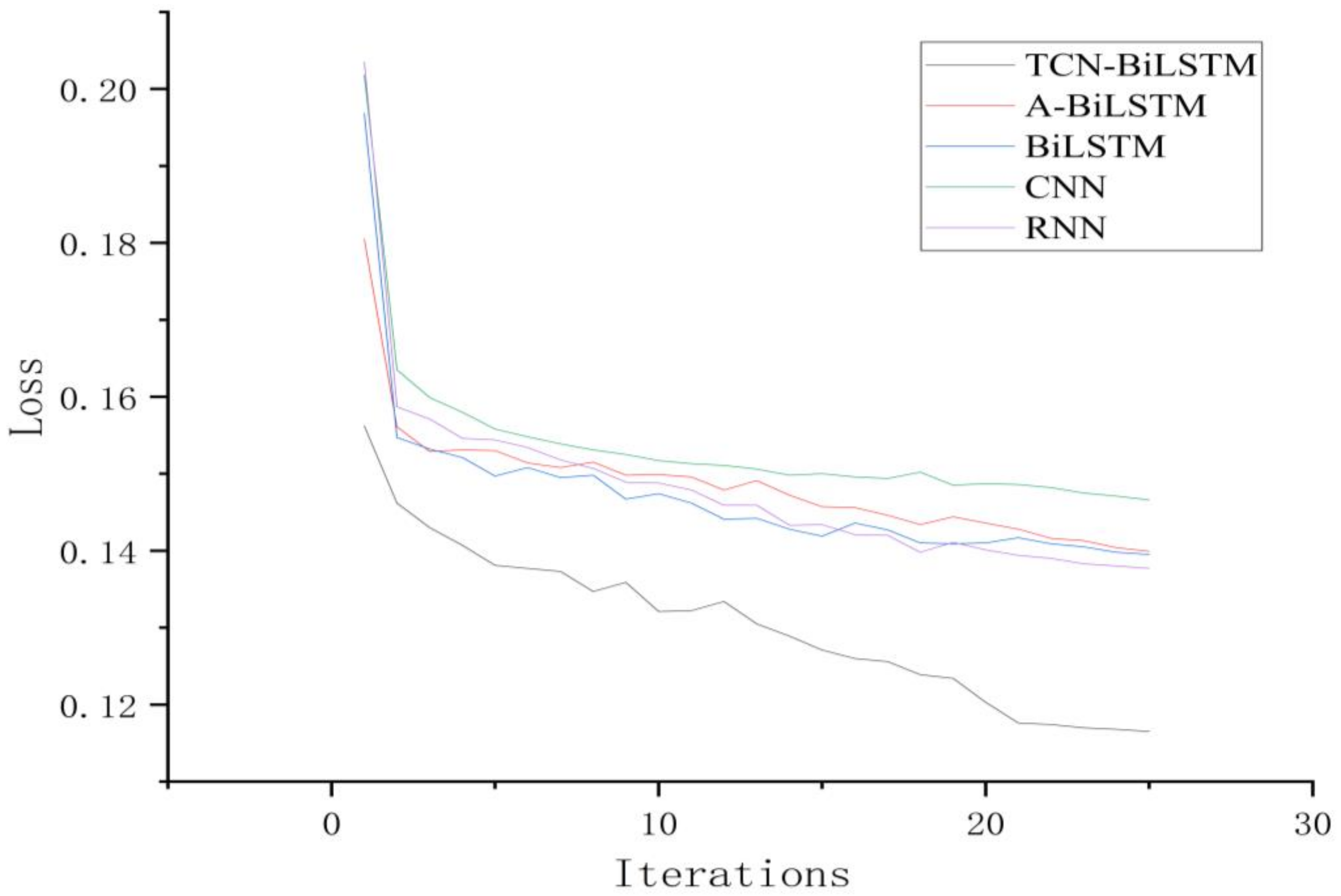
3.5. Experimental Results and Analysis

To validate the effectiveness of the proposed TCN-BiLSTM model for time-series fault prediction tasks, comparative simulation experiments with multiple models were conducted. Under the same dataset and experimental conditions, the proposed model was compared with RNN, CNN, BiLSTM, and A-BiLSTM models [24]. The final experimental results of the test set are illustrated in Figure 7 and Figure 8, showcasing the performance and classification outcomes of various models during multiple iterations of the training process.

An in-depth analysis of the experimental data reveals that all models exhibited a rapid convergence trend during the training phase. Examination of the iterative loss curves indicates that the loss values of the models began to stabilize after approximately 20 iterations, suggesting that these models possess relatively high training efficiency for the given task. Among them, the proposed TCN-BiLSTM model demonstrated superior convergence characteristics, achieving significantly lower loss values within a shorter training duration. This reflects its enhanced capacity for model fitting and generalization. Furthermore, the TCN-BiLSTM model consistently maintained high performance across key evaluation metrics, including Precision, Recall, and F1 Score, underscoring its robustness.

When evaluating the experimental results on the test set, the TCN-BiLSTM model delivered consistently superior classification performance compared to the baseline models. Specifically, it achieved a 20.79% reduction in loss compared to the CNN model, highlighting its remarkable ability to capture temporal dependencies and process sequential data. While CNN excels at extracting localized features, its limited capacity for modeling long-range temporal dependencies constrained its performance in this task. Compared to the BiLSTM model, the TCN-BiLSTM model achieved a 16.67% reduction in loss. Although BiLSTM is proficient at modeling temporal features, its inability to fully leverage long-term dependencies limited its effectiveness, a shortcoming addressed by the introduction of the TCN architecture. Similarly, when compared to the A-BiLSTM model, the TCN-BiLSTM model achieved a 17.09% reduction in loss, and compared to the RNN model, it yielded a 15.54% reduction in loss.

The dilated convolution and batch normalization mechanisms in the TCN-BiLSTM model effectively mitigate the impact of noise in observational data during the predictive phase. In contrast, while the CNN model has certain advantages in extracting local features, its relatively small receptive field makes it more susceptible to being misled by local noise, thereby reducing the accuracy of its predictions. Similarly, although the BiLSTM model is capable of capturing long-term dependencies in time series, it lacks the ability to model multi-scale temporal features.

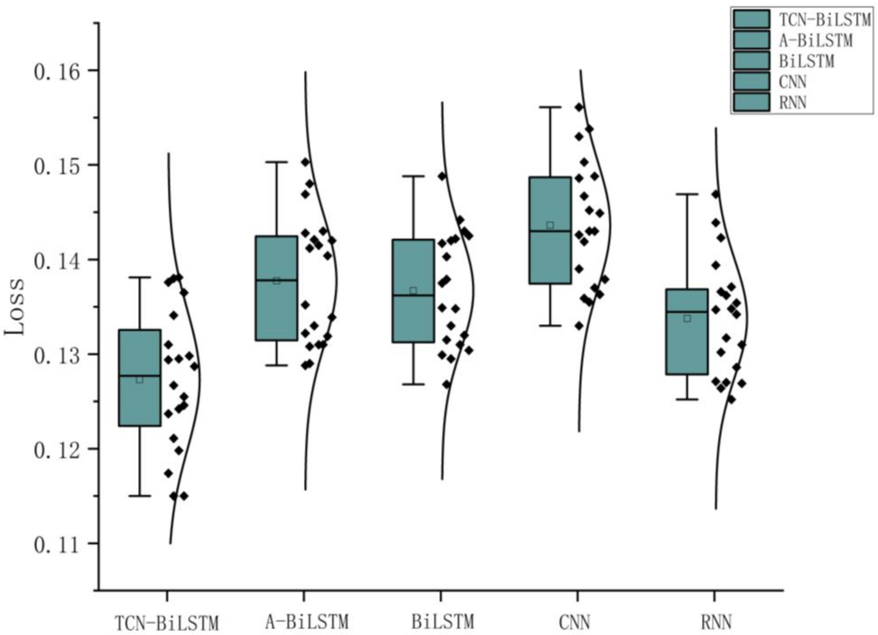
To further validate the performance of the model, significance testing experiments were conducted. Under the same configuration parameters, each model was independently repeated 20 times. The final results of each experiment on the test set are shown in the Figure 9 below.

The paired t-test is a commonly used statistical method primarily designed to assess whether the mean difference between paired observations is statistically significant. In this study, paired t-tests were performed on the loss values of different models to evaluate whether the performance differences between the TCN-BiLSTM model and other comparative models are significant. The final loss values of each model, obtained from 20 identical experimental runs, were paired for comparison, and the corresponding p-values were calculated to determine the statistical significance of the differences.The experimental results are shown in

Table 6. Results of the paired t-test.

p-Values	TCN-BiLSTM	A-BiLSTM	BiLSTM	CNN	RNN
TCN-BiLSTM	/	0.0006	0.0004	0	0.0011
A-BiLSTM	0.0006	/	0.6273	0.0068	0.0999
BiLSTM	0.0004	0.6273	/	0.0016	0.1772
CNN	0	0.0068	0.0016	/	0.0002
RNN	0.0011	0.0999	0.1772	0.0002	/

.

The experimental results demonstrate that the p-values for the performance comparisons between the TCN-BiLSTM model and all other comparative models were consistently less than 0.05. According to statistical standards, when the p-value is smaller than the significance level (commonly set at 0.05), it can be concluded that the observed differences between the two groups are unlikely due to random variations and are statistically significant. This indicates that the TCN-BiLSTM model outperforms all other comparative models in terms of performance.

3.6. Error Classification Case Analysis

In the experiments using the TCN-BiLSTM model for fault classification, although the overall performance outperformed other models, there were still some notable instances of misclassification. By conducting an in-depth analysis of specific misclassified cases, we gained further insights into the limitations of the model.

First, the model misclassified a heat dissipation failure as a random failure. Heat dissipation failure is typically caused by uneven temperature distribution or insufficient heat dissipation characterized by a minimal difference between air temperature and process temperature. It is also closely associated with parameters such as rotational speed and torque. In contrast, a random failure is an extremely rare type of fault (with an occurrence probability of approximately 0.1%) that is completely independent of the operational state of the equipment and occurs randomly. The model may have failed to sufficiently recognize the unique physical characteristics of heat dissipation failure, leading to its misclassification as a random failure. The critical distinction between these two failure types is that heat dissipation failure follows a certain physical mechanism, whereas random failure is entirely stochastic. The model likely struggled to capture the essential differences between these two types of failures.

Second, the model misclassified an overstrain failure as a tool wear failure. Overstrain failure typically occurs when the product of tool wear and torque exceeds a certain threshold, leading to sudden mechanical strain or a violent response of the equipment. In contrast, tool wear failure is a gradual process that progresses more slowly over time. The model may not have effectively captured the temporal dependencies and abrupt characteristics that distinguish overstrain failure from tool wear failure. Moreover, due to the imbalanced dataset, overstrain failure had relatively fewer samples compared to tool wear failure. This imbalance may have caused the model to favor predicting tool wear failure, thereby overlooking the distinguishing features of overstrain failure.

In conclusion, while the comparison of experimental results validated the superior performance of the proposed TCN-BiLSTM model in time-series fault prediction tasks, the analysis of misclassification cases revealed areas for further improvement. The model not only demonstrated higher prediction accuracy but also exhibited faster convergence and stronger adaptability to sequential data. These findings establish the TCN-BiLSTM model as a robust and effective solution for tackling complex time-series prediction challenges, offering a significant advantage over traditional approaches.

3.7. Model Scalability

The TCN-BiLSTM model demonstrates scalability and is capable of adapting to a wide range of real-world application scenarios. For instance, in high-dimensional small-sample problems where the data sample size is limited but the feature dimensions are high, traditional algorithms often struggle to handle such complex situations. The TCN-BiLSTM model, through the following mechanisms, exhibits its potential and scalability when applied to high-dimensional small-sample datasets.

When dealing with high-dimensional datasets, the dilated convolution operation in the TCN-BiLSTM model expands the receptive field, enabling the extraction of multi-level temporal dynamic features over a longer time span. This characteristic allows the model to effectively capture useful signals within the data while reducing the interference of redundant features. The ability to extend the receptive field can be generalized to other high-dimensional small-sample problems. For example, in application scenarios involving large volumes of sensor data, while the number of features might be extremely high, the effective sample size could be quite limited. The scalability of the TCN-BiLSTM model facilitates learning significant features from limited data, thereby enhancing its effectiveness in other high-dimensional small-sample problems.

Through its bidirectional learning mechanism, the TCN-BiLSTM model is able to capture dependencies between previous and subsequent time steps simultaneously. This mechanism contributes to its scalability in small-sample datasets. Small-sample problems are prevalent across various industrial domains, particularly in equipment fault prediction, where certain fault patterns may only manifest during a few time points. By enhancing the model’s contextual understanding of time-series data, BiLSTM enables the extraction of latent long-term dependencies even when the sample size is limited.

To further enhance the model’s adaptability to broader applications, a series of optimization techniques have been incorporated during the network design and training process. These techniques not only improve performance on current tasks but also provide support for future expansions. Batch normalization assists the model in achieving faster and more stable training across diverse tasks, accommodating variations in data distributions. The Leaky ReLU activation function addresses the “dead neuron” problem that may arise when processing high-dimensional data, ensuring model stability in broader application scenarios. The dropout mechanism prevents overfitting while simultaneously enhancing the model’s predictive capabilities on unseen data. With the integration of these techniques, the TCN-BiLSTM model exhibits enhanced generalizability, making it expandable to different domains and datasets, thereby boosting its potential for cross-domain applications.

The TCN-BiLSTM model showcases outstanding scalability, making it applicable to a broader range of industrial fields and complex data types. Through continued algorithmic optimization and technological innovation, the application scenarios and processing capabilities of the model are expected to expand further, driving its adoption across more diverse fields.

4. Conclusions

This study addresses the issue of insufficient accuracy in traditional algorithms and single fault prediction models for time-series fault prediction by proposing a combined prediction model based on an improved temporal convolutional network (TCN) and bidirectional long short-term memory network (BiLSTM), referred to as the TCN-BiLSTM model. By incorporating techniques such as hyperparameter optimization, improved activation functions, and dropout, the model achieves enhanced prediction accuracy and generalization capability. Simulation experiments conducted on a publicly available dataset demonstrate that the proposed model exhibits higher accuracy in time-series fault prediction tasks, along with strong applicability and robustness.

This research provides a novel technical perspective and practical value for the field of time-series fault prediction through the design of an improved algorithm and combined model. Future work will explore the adoption of advanced techniques such as model ensemble methods and transfer learning to further improve the adaptability and generalization of the model, enabling its application to a broader range of time-series fault prediction scenarios.