
Analysis of Surrounding Rock Stability Based on Refined Geological and Mechanical Parameter Modeling—A Case Study
Abstract
1. Introduction
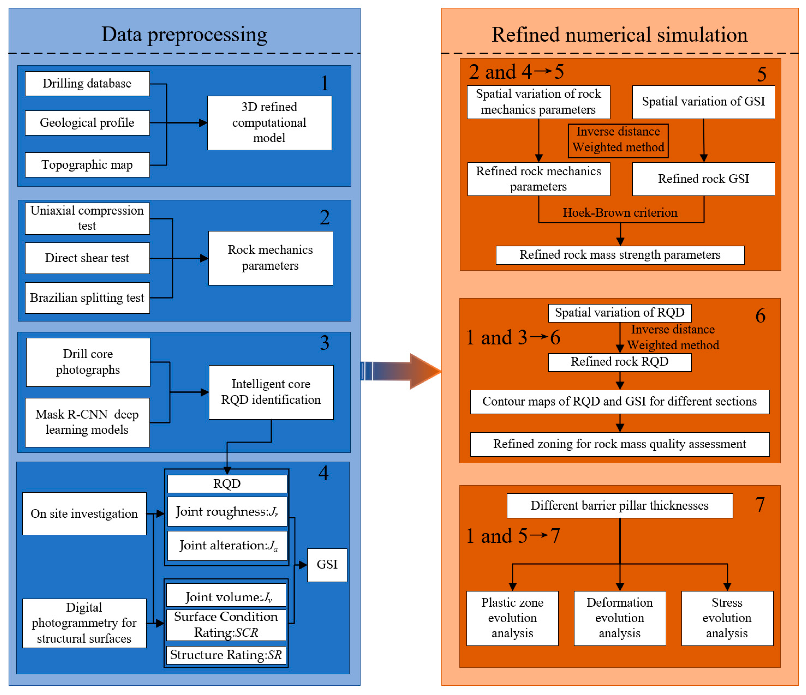
2. Methodology
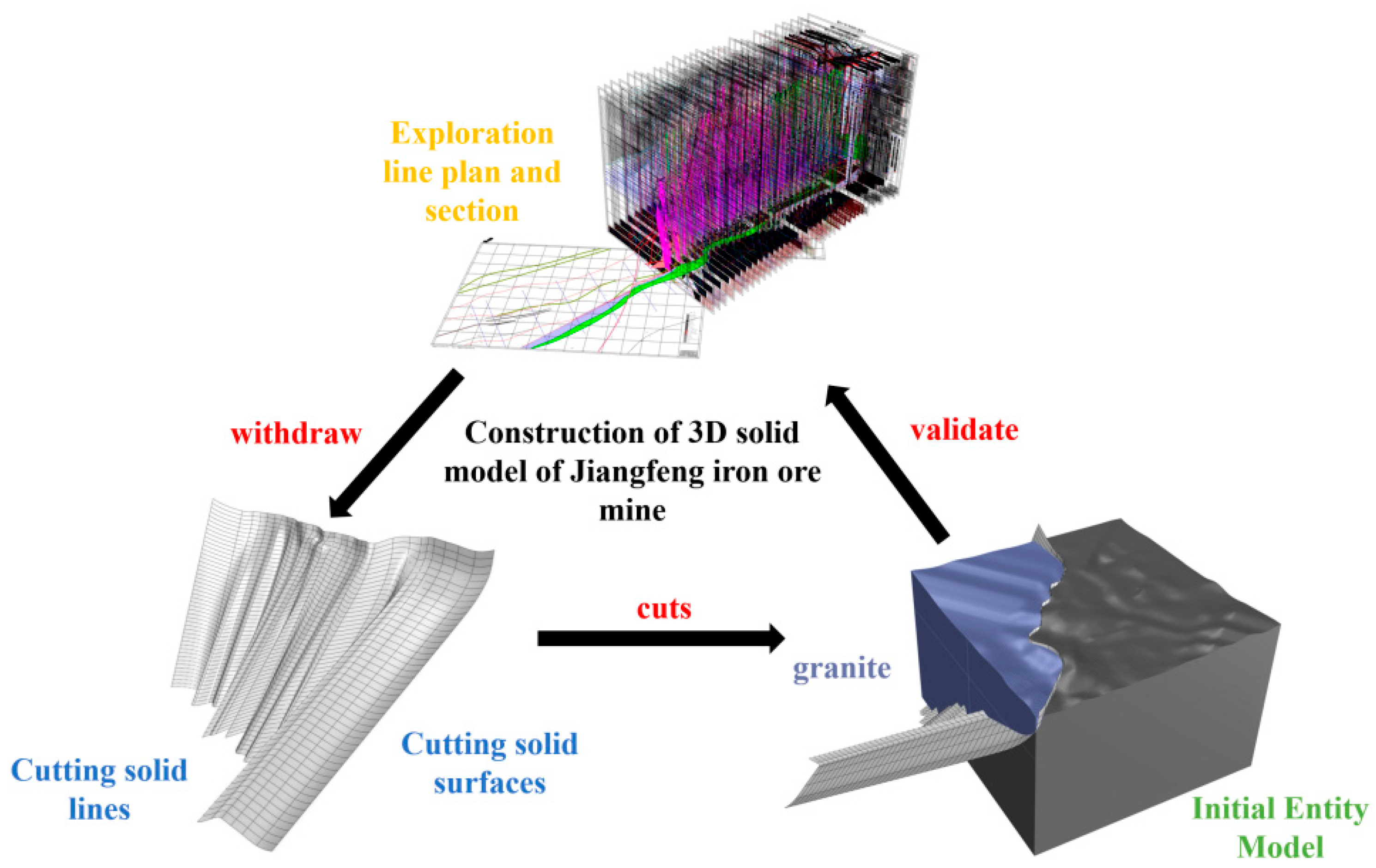
2.1. Construction of a Refined 3D Computational Model
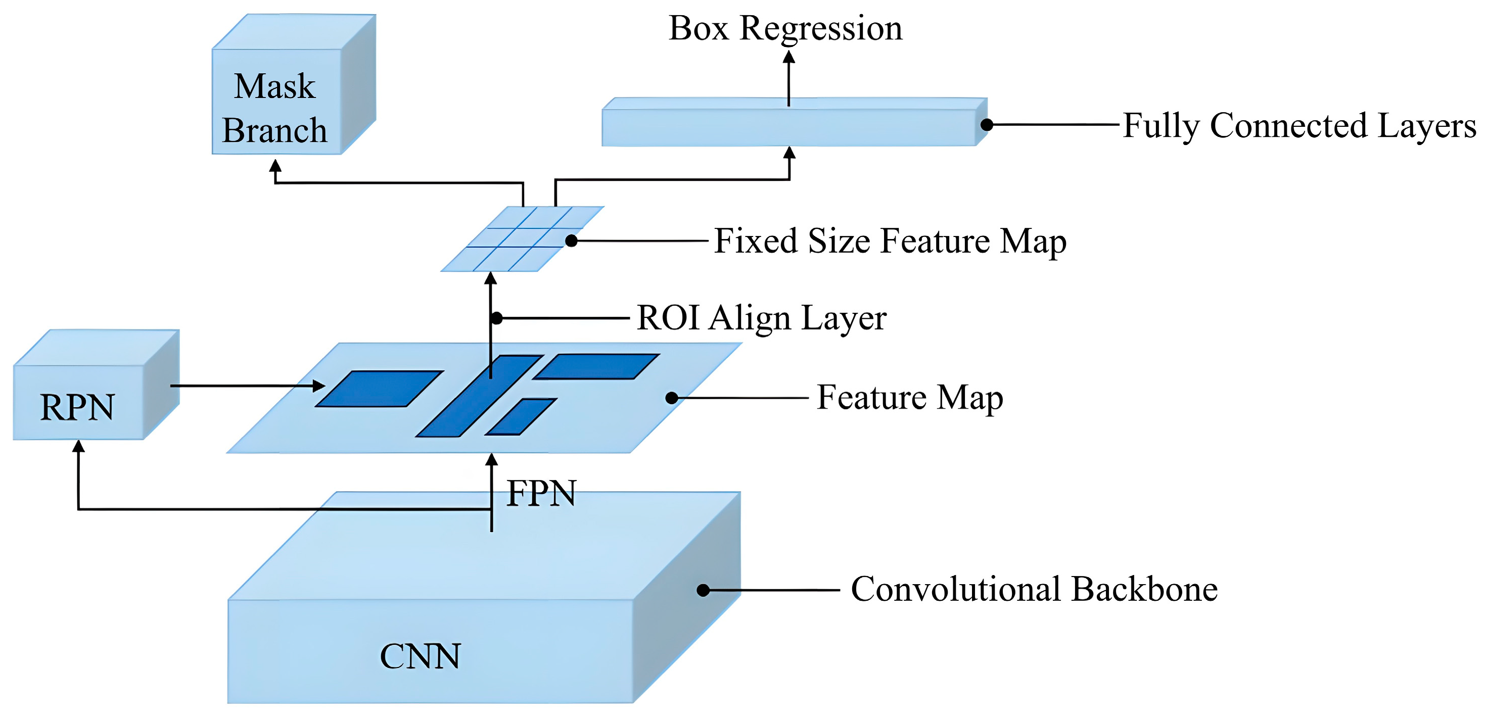
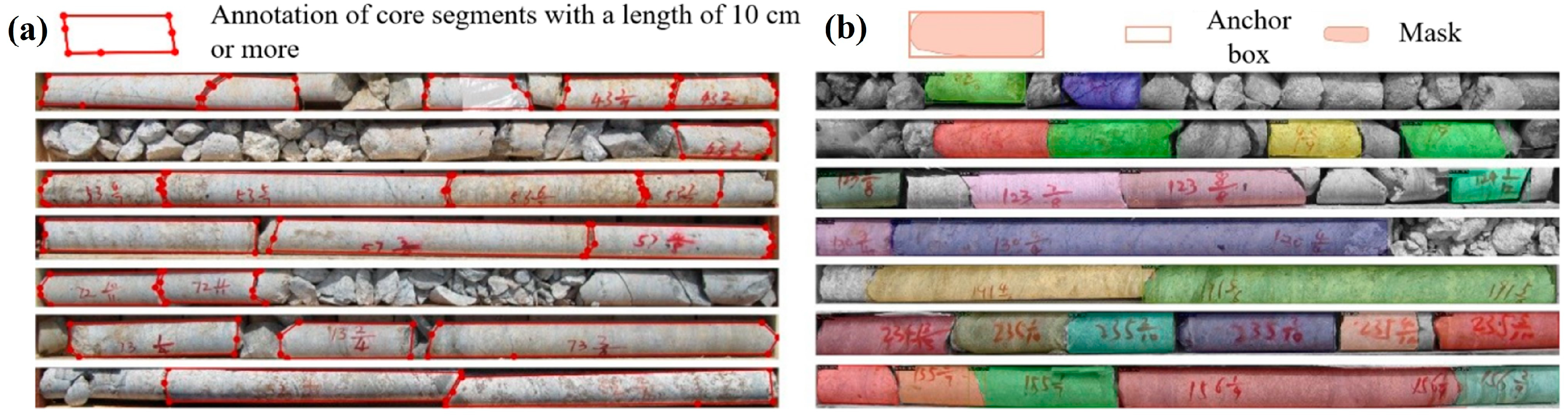
2.2. Calculation Method of Rock Mass Evaluation Indices
2.3. Calculation of Refined Rock Mass Strength Parameters
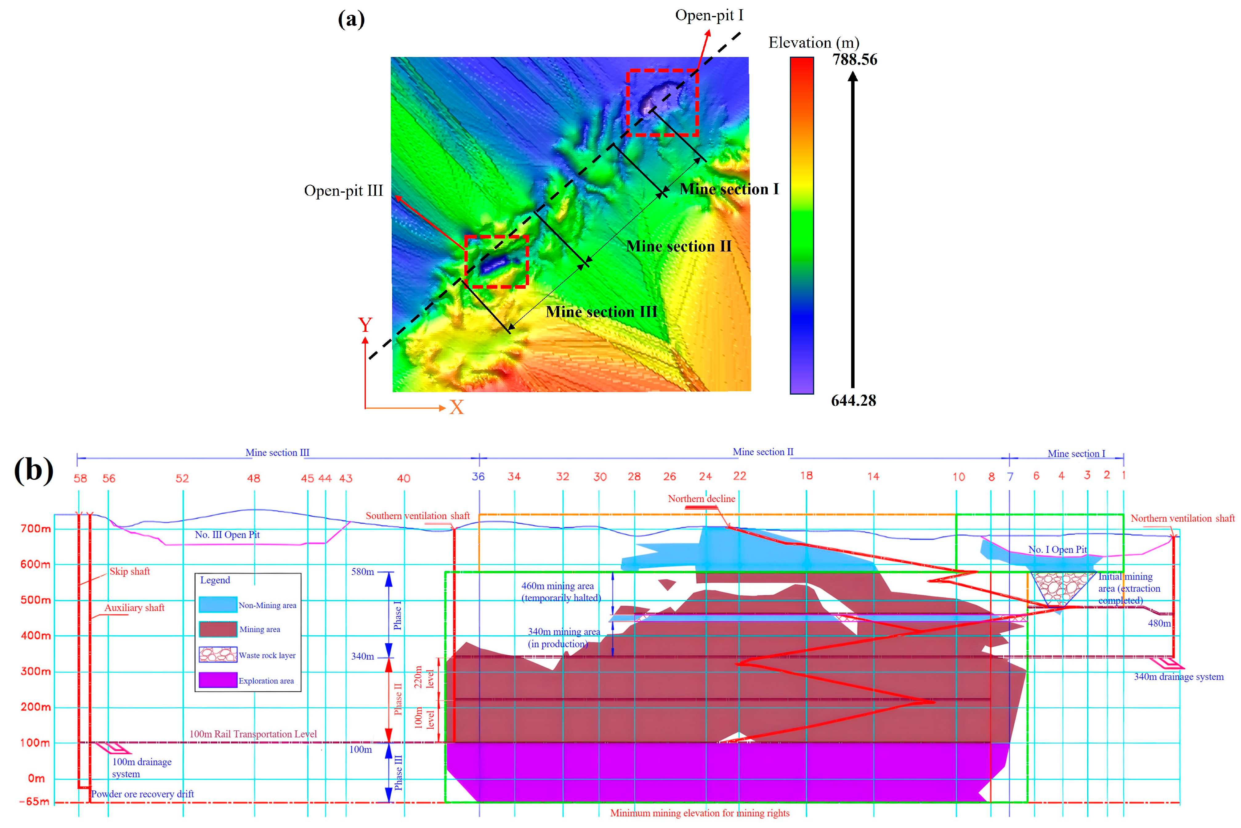
3. Engineering Background
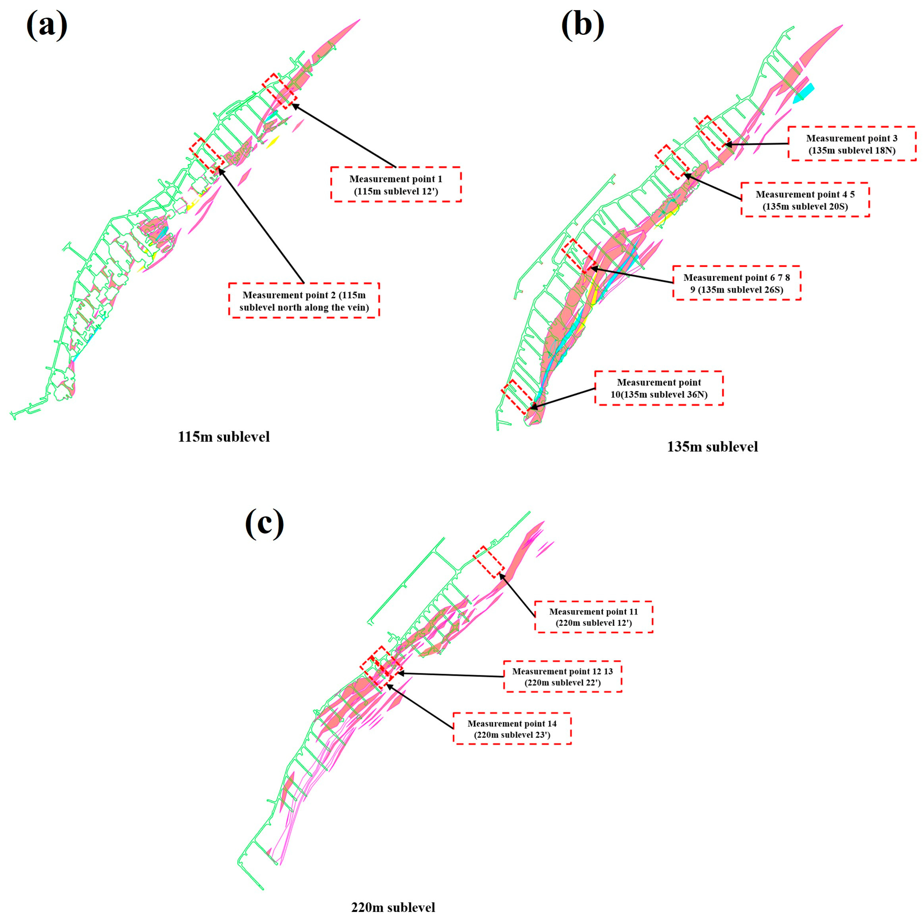
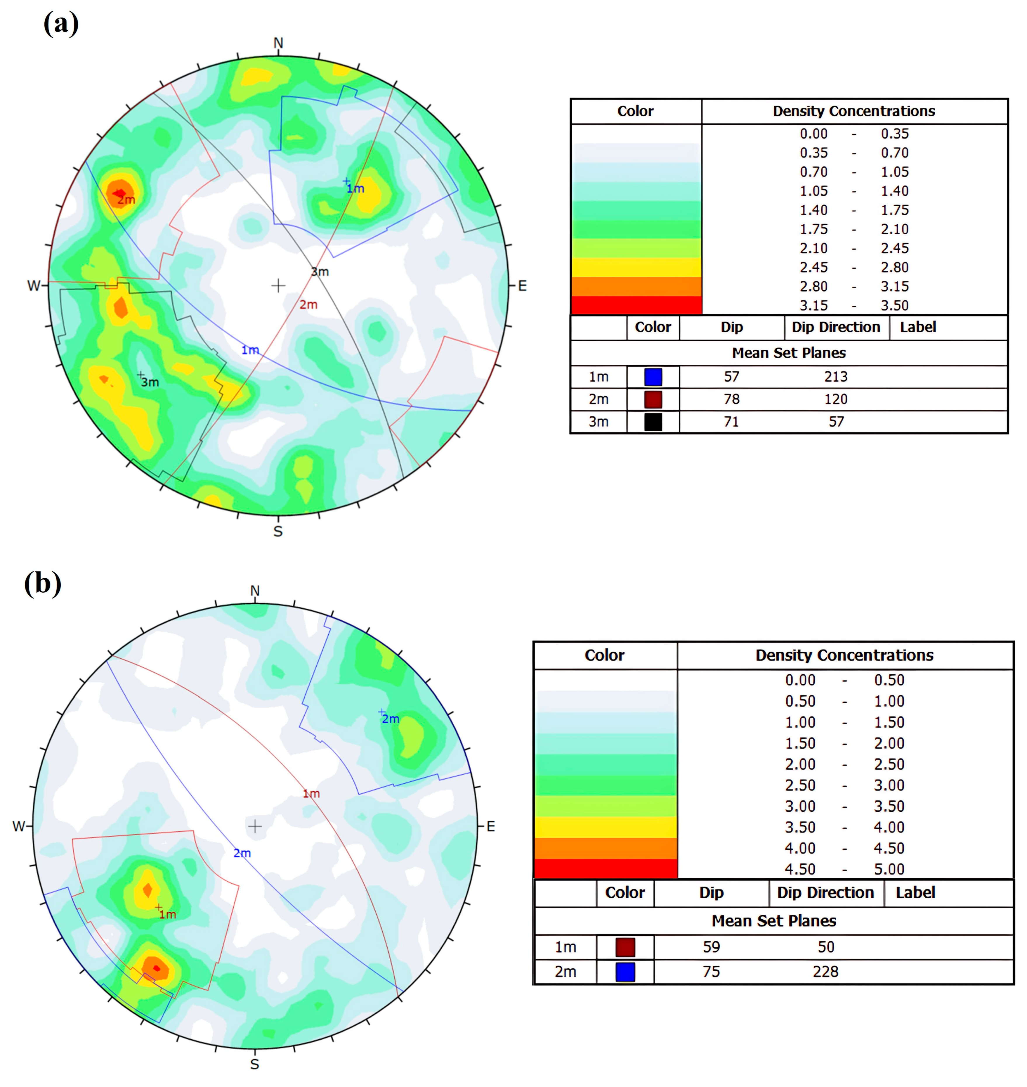
4. Acquisition of Structural Surface Parameters
5. Rock Mass Quality Evaluation
5.1. Refined RQD Evaluation Zoning
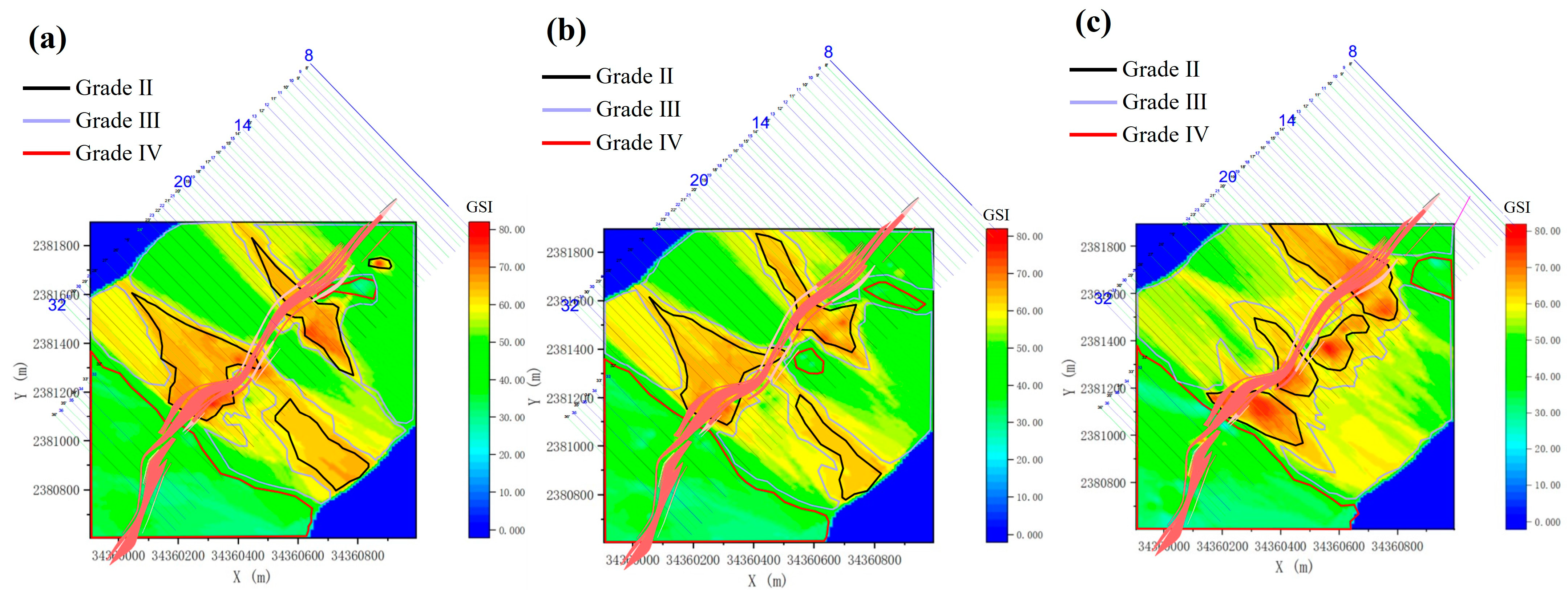
5.2. Refined GSI Evaluation Zoning
6. Stability Analysis of Surrounding Rock Based on Refined Modeling
6.1. Refined Computational Model
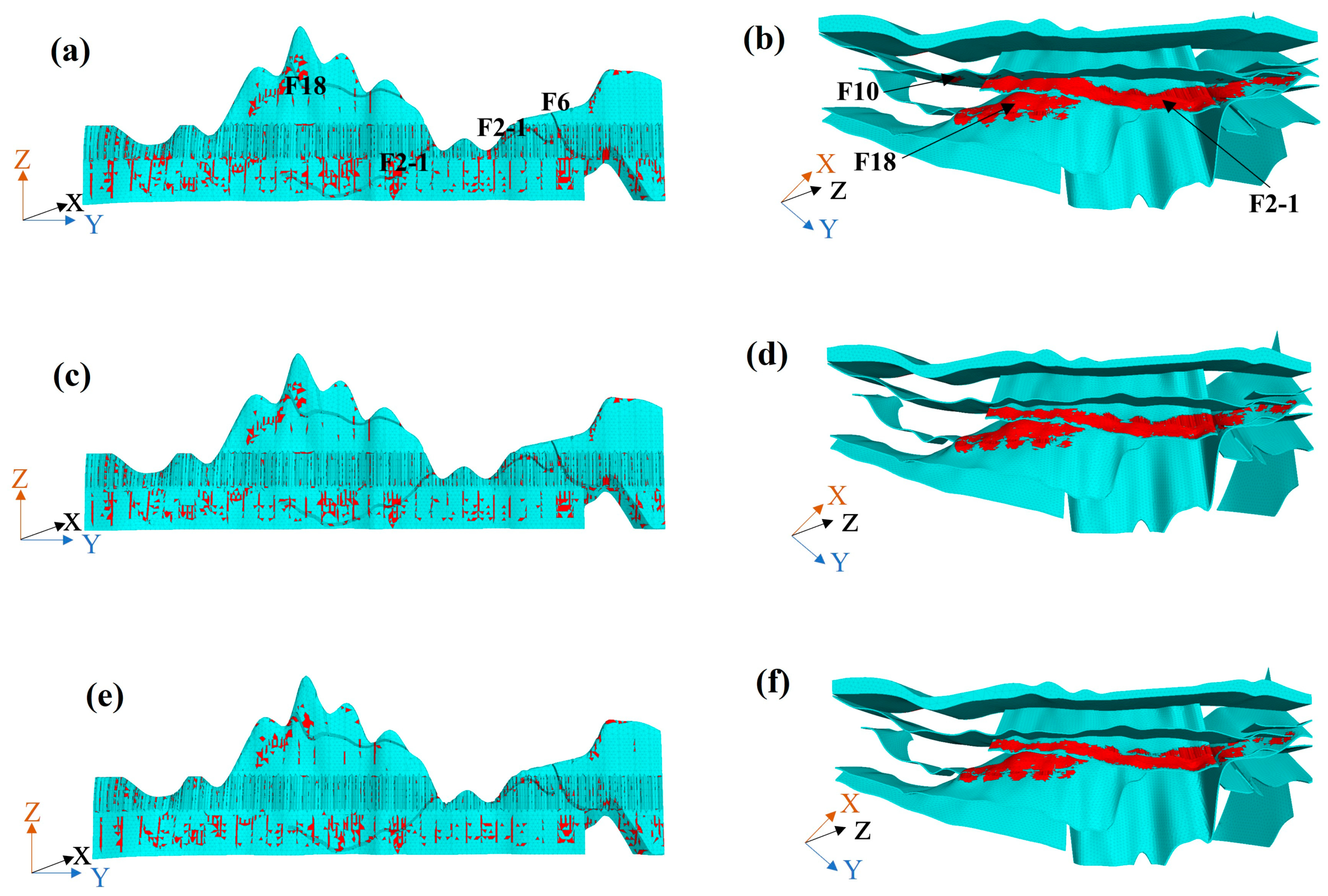
6.2. Analysis of Plastic Zone Evolution
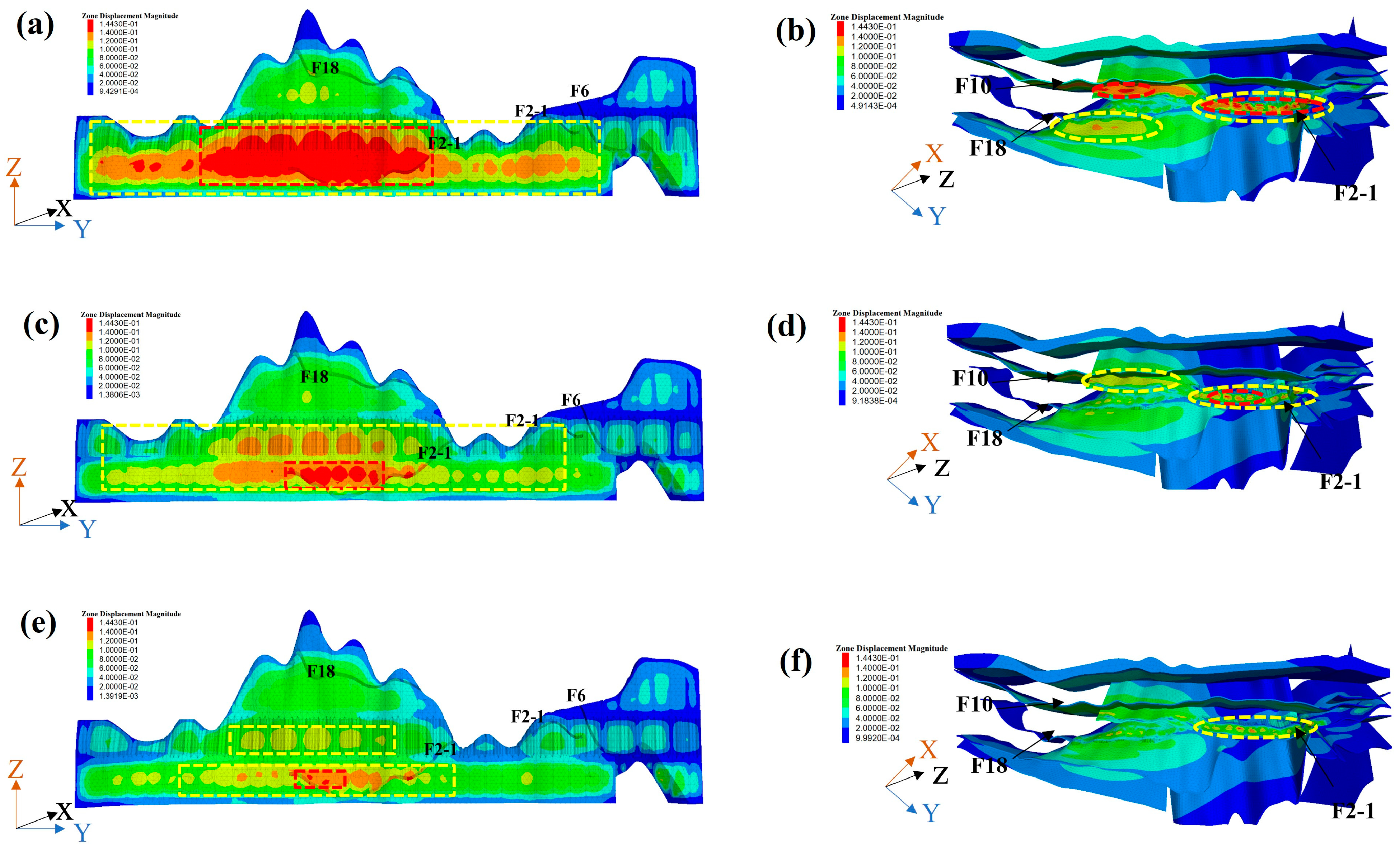
6.3. Analysis of Deformation Evolution
6.4. Analysis of Stress Evolution
6.4.1. Stress Analysis of KZ1 Profile
6.4.2. Stress Analysis of KH1 Profile
7. Conclusions
Author Contributions
Funding
Data Availability Statement
Conflicts of Interest
References
- Wilkinson, J.J. Triggers for the Formation of Porphyry Ore Deposits in Magmatic Arcs. Nat. Geosci. 2013, 6, 917–925. [Google Scholar] [CrossRef]
- Ankah, M.L.Y.; Sunkpal, D.T.; Zhao, X.; Kulatilake, P.H.S.W. Role of Heterogeneity on Joint Size Effect, and Influence of Anisotropy and Sampling Interval on Rock Joint Roughness Quantification. Geomech. Geophys. Geo-Energ. Geo-Resour. 2022, 8, 101. [Google Scholar] [CrossRef]
- Ma, H.-P.; Daud, N.N.N. Jointed Rock Failure Mechanism: A Method of Heterogeneous Grid Generation for DDARF. Appl. Sci. 2022, 12, 6095. [Google Scholar] [CrossRef]
- Jian-po, L.; Shi-da, X.; Yuan-hui, L. Analysis of Rock Mass Stability According to Power-Law Attenuation Characteristics of Acoustic Emission and Microseismic Activities. Tunn. Undergr. Space Technol. 2019, 83, 303–312. [Google Scholar] [CrossRef]
- Li, S.C.; Wu, J.; Xu, Z.H.; Zhou, L.; Zhang, B. A Possible Prediction Method to Determine the Top Concealed Karst Cave Based on Displacement Monitoring during Tunnel Construction. Bull. Eng. Geol. Environ. 2019, 78, 341–355. [Google Scholar] [CrossRef]
- Guo, Y.J. The Stability Research of Highway Bedded Rock Slope Based on the Stress Monitoring. AMM 2013, 351–352, 1253–1256. [Google Scholar] [CrossRef]
- Jia, H.; Yan, B.; Yang, Z.; Yilmaz, E. Identification of Goaf Instability under Blasting Disturbance Using Microseismic Monitoring Technology. Geomech. Geophys. Geo-Energ. Geo-Resour. 2023, 9, 142. [Google Scholar] [CrossRef]
- Xu, Y.; Yue, T.; Wu, B.; Wang, Q.; Cheng, C.; Xu, Z. Dynamic Tensile Properties of Sandstone under Coupling Effects of Water Chemical Corrosion and Freeze-Thaw Cycles at Sub-Zero Temperatures. Constr. Build. Mater. 2025, 458, 139734. [Google Scholar] [CrossRef]
- Korzeniowski, W.; Skrzypkowski, K.; Herezy, Ł. Laboratory Method for Evaluating the Characteristics of Expansion Rock Bolts Subjected to Axial Tension/Laboratoryjna Metoda Badania Charakterystyk Kotew Rozprężnych Poddanych Rozciąganiu Osiowemu. Arch. Min. Sci. 2015, 60, 209–224. [Google Scholar] [CrossRef]
- Yang, P.; Zhang, S.; Liu, C. Study on Shear Failure Process and Zonal Disintegration Mechanism of Roadway under High Ground Stress: A Numerical Simulation via a Strain-Softening Plastic Model and the Discrete Element Method. Appl. Sci. 2024, 14, 4106. [Google Scholar] [CrossRef]
- Yang, W.; Geng, Y.; Zhou, Z.; Li, L.; Ding, R.; Wu, Z.; Zhai, M. True Triaxial Hydraulic Fracturing Test and Numerical Simulation of Limestone. J. Cent. S. Univ. 2020, 27, 3025–3039. [Google Scholar] [CrossRef]
- Xu, J.; Zhu, W.; Xu, J.; Wu, J.; Li, Y. High-Intensity Longwall Mining-Induced Ground Subsidence in Shendong Coalfield, China. Int. J. Rock Mech. Min. Sci. 2021, 141, 104730. [Google Scholar] [CrossRef]
- Huo, X.; Jiang, Y.; Wei, W.; Qiu, X.; Yu, Z.; Nong, J.; Li, Q. Three-Dimensional Finite Element Simulation and Reconstruction of Jointed Rock Masses for Bench Blasting. Simul. Modell. Pract. Theory 2024, 135, 102975. [Google Scholar] [CrossRef]
- Gu, Z.; Cao, M. Analysis of Unstable Block by Discrete Element Method during Blasting Excavation of Fractured Rock Mass in Underground Mine. Heliyon 2023, 9, e22558. [Google Scholar] [CrossRef] [PubMed]
- Li, J.; Gao, Y.; Yang, T.; Zhang, P.; Zhao, Y.; Deng, W.; Liu, H.; Liu, F. Integrated Simulation and Monitoring to Analyze Failure Mechanism of the Anti-Dip Layered Slope with Soft and Hard Rock Interbedding. Int. J. Min. Sci. Technol. 2023, 33, 1147–1164. [Google Scholar] [CrossRef]
- Zhuang, D.; Ning, Z.; Argilaga, A.; Ma, K.; Tang, C.; Li, J.; Xu, W.; Zhang, S. Stability Analysis of Jointed Rock Mass in Large Underground Caverns Based on Multi-Scale Analysis Method. Transp. Geotech. 2023, 42, 101109. [Google Scholar] [CrossRef]
- Wang, L.; Zhang, X.; Yin, S.; Zhang, X.; Jia, Y.; Kong, H. Evaluation of Stope Stability and Displacement in a Subsidence Area Using 3Dmine–Rhino3D–FLAC3D Coupling. Minerals 2022, 12, 1202. [Google Scholar] [CrossRef]
- Zhang, Q. A Shear Strength Criterion of Rock Joints under Dynamic Normal Load. Int. J. Rock Mech. Min. Sci. 2025, 186, 106002. [Google Scholar] [CrossRef]
- Aliyu, M.; Shang, J.; Murphy, W.; Lawrence, J.; Collier, R.; Kong, F.; Zhao, Z. Assessing the Uniaxial Compressive Strength of Extremely Hard Cryptocrystalline Flint. Int. J. Rock Mech. Min. Sci. 2019, 113, 310–321. [Google Scholar] [CrossRef]
- Zeng, B.; Qiu, G.; Huang, H.; Guo, Y.; Xu, E.; Gui, J.; Li, J. Study on the Mechanical Properties and Failure Mechanism of a Multi-Lithologic Layered Rock Mass. Heliyon 2025, 11, e41233. [Google Scholar] [CrossRef] [PubMed]
- He, K.; Gkioxari, G.; Dollar, P.; Girshick, R. Mask R-CNN. In Proceedings of the 2017 IEEE International Conference on Computer Vision (ICCV), Venice, Italy, 22–29 October 2017; IEEE: Piscataway, NJ, USA; pp. 2980–2988. [Google Scholar]
- Ren, S.; He, K.; Girshick, R.; Sun, J. Faster R-CNN: Towards Real-Time Object Detection with Region Proposal Networks. IEEE Trans. Pattern Anal. Mach. Intell. 2017, 39, 1137–1149. [Google Scholar] [CrossRef]
- Neubeck, A.; Van Gool, L. Efficient Non-Maximum Suppression. In Proceedings of the 18th International Conference on Pattern Recognition (ICPR’06), Hong Kong, China, 20–24 August 2006; IEEE: Piscataway, NJ, USA; pp. 850–855. [Google Scholar]
- Li, J.; Yang, T.; Liu, F.; Zhao, Y.; Liu, H.; Deng, W.; Gao, Y.; Li, H. Modeling Spatial Variability of Mechanical Parameters of Layered Rock Masses and Its Application in Slope Optimization at the Open-Pit Mine. Int. J. Rock Mech. Min. Sci. 2024, 181, 105859. [Google Scholar] [CrossRef]
- Russo, G. A New Rational Method for Calculating the GSI. Tunn. Undergr. Space Technol. 2009, 24, 103–111. [Google Scholar] [CrossRef]
- Sonmez, H.; Ulusay, R. Modifications to the Geological Strength Index (GSI) and Their Applicability to Stability of Slopes. Int. J. Rock Mech. Min. Sci. 1999, 36, 743–760. [Google Scholar] [CrossRef]
- Hoek, E.; Carter, T.; Diederichs, M. Quantification of the Geological Strength Index Chart. In Proceedings of the 47th US Rock. Mechanics/Geomechanics Symposium, San Francisco, CA, USA, 23–26 June 2013; Volume 3, pp. 1757–1764. [Google Scholar]
- Hencher, S. Practical Rock Mechanics; CRC Press: Boca Raton, FL, USA, 2015. [Google Scholar]
- Hoek, E.; Brown, E.T. Underground Excavations in Rock; CRC Press: London, UK, 1980. [Google Scholar]
- Hoek, E.; Brown, E.T. Empirical Strength Criterion for Rock Masses. J. Geotech. Geoenviron. Eng. 1980, 106, 1013–1035. [Google Scholar] [CrossRef]
- Hoek, E.; Carranza-Torres, C.; Corkum, B. Hoek-Brown Failure Criterion—2002 Edition. In Proceedings of the 5th North American Rock Mechanics Symposium and 17th Tunneling Association of Canada Conference, Toronto, ON, Canada, 7–10 July 2002; pp. 267–271. [Google Scholar]
- Bieniawski, Z.T. Engineering Rock Mass Classifications: A Complete Manual for Engineers and Geologists in Mining, Civil, and Petroleum Engineering; John Wiley & Sons: New York, NY, USA, 1989. [Google Scholar]
- Blachowski, J.; Ellefmo, S.L. Mining Ground Deformation Estimation Based on Pre-Processed InSAR Open Data—A Norwegian Case Study. Minerals 2023, 13, 328. [Google Scholar] [CrossRef]
- Wang, Y.-J.; Zhao, L.-S.; Xu, Y.-S. Analysis of Characteristics of Roof Fall Collapse of Coal Mine in Qinghai Province, China. Appl. Sci. 2022, 12, 1184. [Google Scholar] [CrossRef]
- Wang, J.; Li, M.; Wang, Z.; Li, Z.; Zhang, H.; Song, S. The Influence of Inter-Band Rock on Rib Spalling in Longwall Panel with Large Mining Height. Int. J. Min. Sci. Technol. 2024, 34, 427–442. [Google Scholar] [CrossRef]
- Sakhno, I.; Sakhno, S. Numerical Studies of Floor Heave Mechanism and the Effectiveness of Grouting Reinforcement of Roadway in Soft Rock Containing the Mine Water. Int. J. Rock Mech. Min. Sci. 2023, 170, 105484. [Google Scholar] [CrossRef]
- Wang, Q.; Wang, Y.; Jiang, B.; Gao, H.; Ma, F.; Zhai, D.; Cai, S. Testing Method of Rock Structural Plane Using Digital Drilling. J. Rock Mech. Geotech. Eng. 2024, 16, 2563–2578. [Google Scholar] [CrossRef]
- Buyer, A.; Aichinger, S.; Schubert, W. Applying Photogrammetry and Semi-Automated Joint Mapping for Rock Mass Characterization. Eng. Geol. 2020, 264, 105332. [Google Scholar] [CrossRef]


| Rock Lithology | Density (kg/m3) | Uniaxial Compressive Strength (MPa) | Cohesion (MPa) | Friction Angle (°) | Elastic Modulus (GPa) | Poisson’s Ratio | GSI | mi |
|---|---|---|---|---|---|---|---|---|
| Non-ore skarn (surrounding rock) | 2890 | 86.08 | 6.83 | 48.16 | 15.1 | 0.26 | 55 | 9 |
| Ore-bearing skarn (ore body) | 4020 | 115.89 | 12.02 | 53.13 | 21.1 | 0.27 | 62 | 19 |
| Diabase | 2690 | 85.2 | 10.95 | 44.1 | 32.5 | 0.29 | 56 | 19 |
| Schist | 2820 | 58.3 | 4.69 | 43.78 | 23.8 | 0.28 | 50 | 6 |
| Granulite | 2720 | 91.3 | 7.83 | 45.28 | 25.5 | 0.26 | 52 | 33 |
| Syenite | 2700 | 63.86 | 2.35 | 44.60 | 18.8 | 0.26 | 55 | 28 |
| Amphibolite | 2880 | 122.9 | 3.40 | 47.60 | 3.59 | 0.2 | 64 | 28 |
| Granite | 2580 | 74 | 8.1 | 43.40 | 3.78 | 0.26 | 60 | 33 |
| Rock Mass Lithology | Tensile Strength (MPa) | Elastic Modulus (GPa) | Friction Angle (°) | Cohesion (MPa) | Poisson’s Ratio | Rock Mass Quality Classification |
|---|---|---|---|---|---|---|
| Non-ore skarn (surrounding rock) | 0.88 | 12.74 | 32.23 | 0.79 | 0.26 | III |
| Ore-bearing skarn (ore body) | 1.36 | 19.21 | 39.55 | 1.44 | 0.27 | III |
| Diabase | 0.89 | 13.04 | 39.11 | 0.94 | 0.29 | III |
| Schist | 0.65 | 7.64 | 23.55 | 0.49 | 0.28 | IV |
| Granulite | 0.92 | 10.72 | 42.25 | 1.04 | 0.26 | III |
| Syenite | 0.87 | 10.66 | 39.59 | 0.93 | 0.26 | III |
| Amphibolite | 1.16 | 24.82 | 48.5 | 1.53 | 0.2 | III |
| Granite | 0.93 | 15.30 | 44.94 | 1.12 | 0.26 | II |
| Fault breccia zone | 0.31 | 2.95 | 22.75 | 0.23 | 0.26 | / |
| Sublevel | Grade II | Grade III | Grade IV |
|---|---|---|---|
| 115 Sublevel | Exploration lines 19~22 Exploration lines 25~26 | Exploration lines 26~27 | Exploration lines 13~19 Exploration lines 22~25 Exploration lines 27~31 |
| 135 Sublevel | Exploration lines 18~22 Exploration lines 27~31 | Exploration lines 22~27 | Exploration lines 13~18 Exploration lines 31~36 |
| 220 Sublevel | Exploration lines 16~26 Exploration lines 29~32 | Exploration lines 26~29 | Exploration lines 13~16 Exploration lines 32~36 |
| Sublevel | Grade II | Grade III | Grade IV |
|---|---|---|---|
| 115 Sublevel | Exploration lines 19~21 Exploration lines 24~31 | Exploration lines 13~19 Exploration lines 21~24 | Exploration lines 31~36 |
| 135 Sublevel | Exploration lines 19~23 Exploration lines 24~31 | Exploration lines 13~19 Exploration lines 23~24 | Exploration lines 31~36 |
| 220 Sublevel | Exploration lines 15~20 Exploration lines 24~27 Exploration lines 28~31 | Exploration lines 13~15 Exploration lines 20~24 Exploration lines 27~28 | Exploration lines 31~36 |
| Plan | Operating Condition | Mining Sequence | Plan |
|---|---|---|---|
| 1 | No isolation pillar | Unidirectional mining | 1 |
| 2 | Isolation pillar thickness of 10 m | Unidirectional mining | 2 |
| 3 | Isolation pillar thickness of 20 m | Unidirectional mining | 3 |
| Isolation Pillar Thickness (m) | Range of Minimum Principal Stress (Pa) | Range of Maximum Principal Stress (Pa) |
|---|---|---|
| 0 | −6.6922 × 10⁷~1.4813 × 10⁴ | −2.3786 × 10⁷~1.0002 × 10⁶ |
| 10 | −6.0441 × 10⁷~9.3152 × 10⁴ | −2.1936 × 10⁷~9.2852 × 10⁵ |
| 20 | −4.5129 × 10⁷~2.6060 × 10⁴ | −2.1475 × 10⁷~8.4438 × 10⁵ |
| Isolation Pillar Thickness (m) | Range of Minimum Principal Stress (Pa) | Range of Maximum Principal Stress (Pa) |
|---|---|---|
| 0 | −1.5899 × 10⁵~−5.3325 × 10⁷ | −2.0863 × 10⁷~8.7776 × 10⁵ |
| 10 | −1.4940 × 10⁵~−5.1028 × 10⁷ | −2.1413 × 10⁷~8.6008 × 10⁵ |
| 20 | −1.4426 × 10⁵~−4.8914 × 10⁷ | −2.1055 × 10⁷~8.0903 × 10⁵ |
Disclaimer/Publisher’s Note: The statements, opinions and data contained in all publications are solely those of the individual author(s) and contributor(s) and not of MDPI and/or the editor(s). MDPI and/or the editor(s) disclaim responsibility for any injury to people or property resulting from any ideas, methods, instructions or products referred to in the content. |
© 2025 by the authors. Licensee MDPI, Basel, Switzerland. This article is an open access article distributed under the terms and conditions of the Creative Commons Attribution (CC BY) license (https://creativecommons.org/licenses/by/4.0/).
Share and Cite
Chai, G.; Zhao, Y.; Yang, T.; Zhao, Q.; Jiao, S.; Li, J. Analysis of Surrounding Rock Stability Based on Refined Geological and Mechanical Parameter Modeling—A Case Study. Appl. Sci. 2025, 15, 1465. https://doi.org/10.3390/app15031465
Chai G, Zhao Y, Yang T, Zhao Q, Jiao S, Li J. Analysis of Surrounding Rock Stability Based on Refined Geological and Mechanical Parameter Modeling—A Case Study. Applied Sciences. 2025; 15(3):1465. https://doi.org/10.3390/app15031465
Chicago/Turabian StyleChai, Guangzhi, Yong Zhao, Tianhong Yang, Qianbai Zhao, Shihui Jiao, and Jinduo Li. 2025. "Analysis of Surrounding Rock Stability Based on Refined Geological and Mechanical Parameter Modeling—A Case Study" Applied Sciences 15, no. 3: 1465. https://doi.org/10.3390/app15031465
APA StyleChai, G., Zhao, Y., Yang, T., Zhao, Q., Jiao, S., & Li, J. (2025). Analysis of Surrounding Rock Stability Based on Refined Geological and Mechanical Parameter Modeling—A Case Study. Applied Sciences, 15(3), 1465. https://doi.org/10.3390/app15031465