
Insights from Optimized Non-Landslide Sampling and SHAP Explainability for Landslide Susceptibility Prediction


Abstract
1. Introduction
2. Study Area and Data Sources
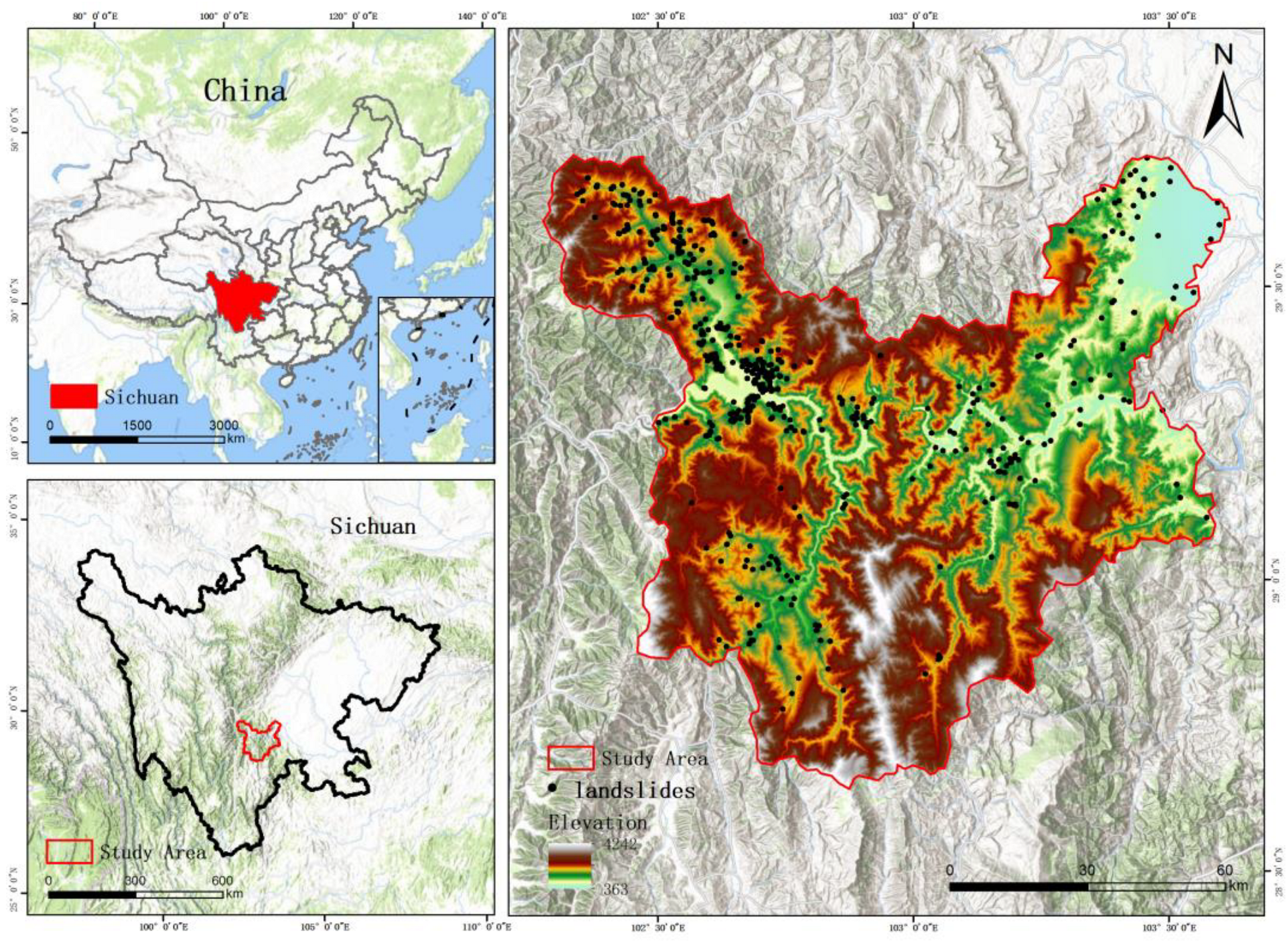
2.1. Study Area
2.2. Landslide Inventory
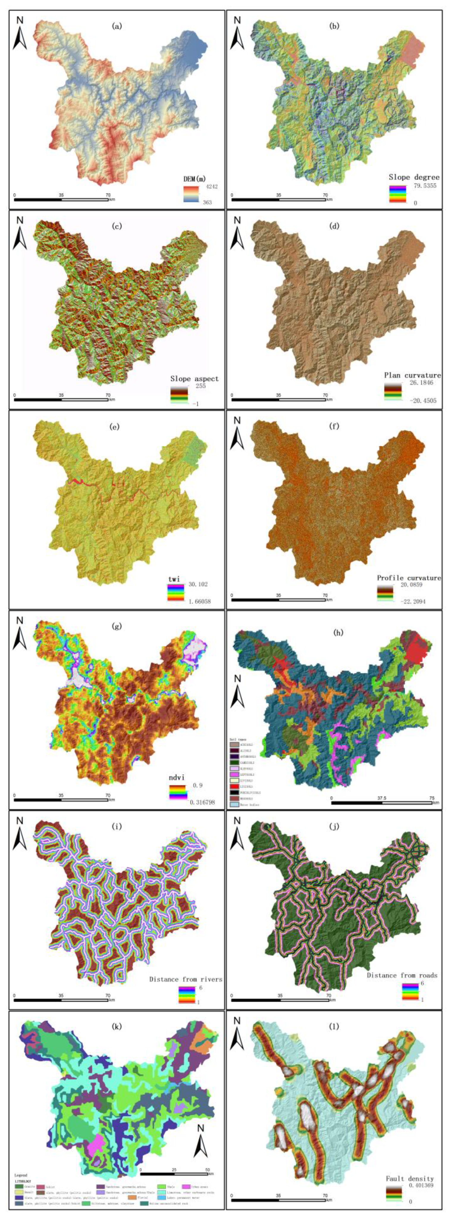
2.3. Landslide Conditioning Factors
2.3.1. Topographic Factors
2.3.2. Environmental Factors
2.3.3. Geological Factors
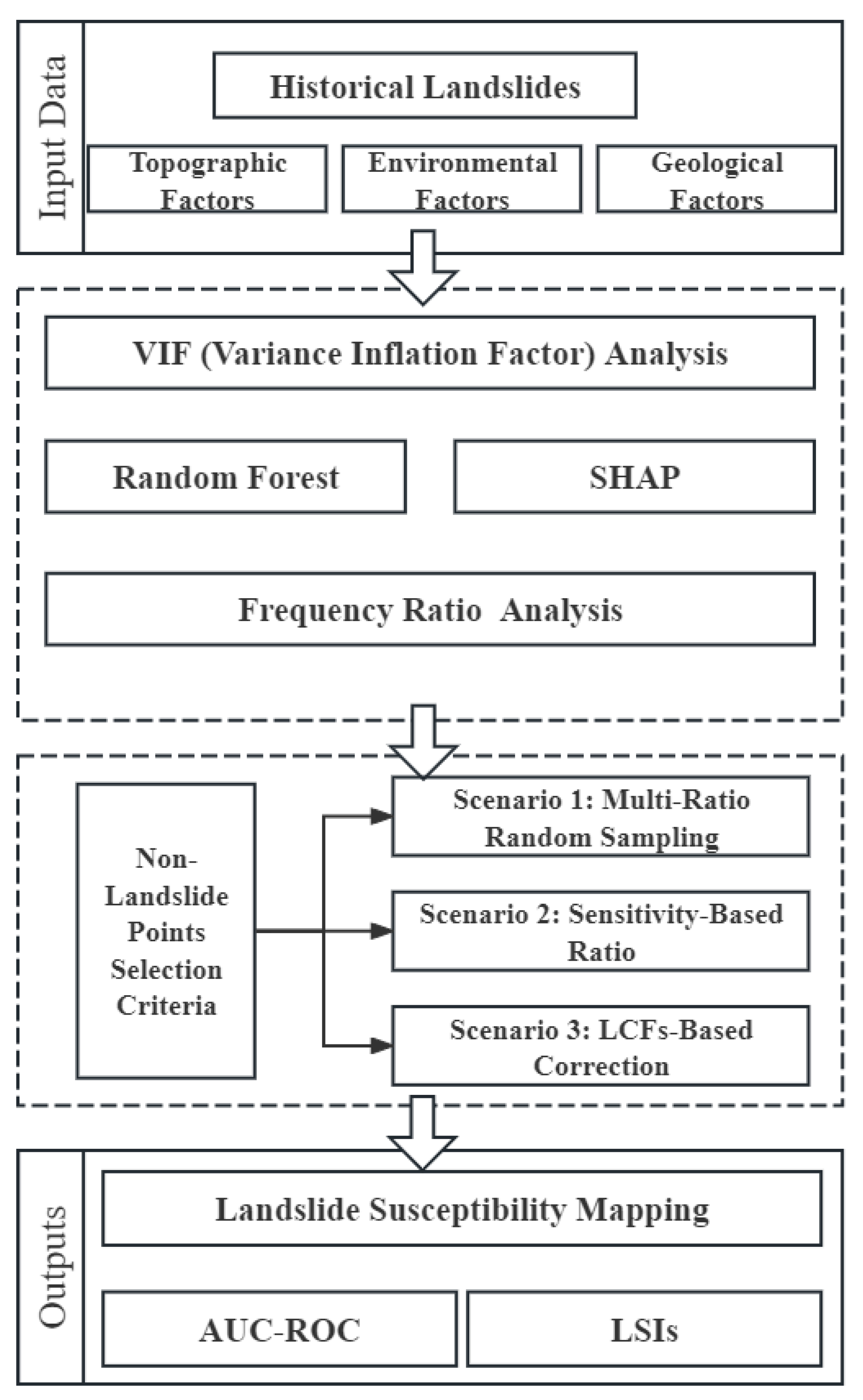
3. Methodology
3.1. Three Non-Landslide Sampling Methods
3.2. Initial LSP Modeling—Random Forest
3.3. SHAP (SHapley Additive exPlanation)
3.4. Model Evaluation
3.4.1. Frequency Ratio Analysis
3.4.2. Receiver Operating Characteristic Curve
4. Analysis
4.1. Relationship Between LCFs and Historical Landslides
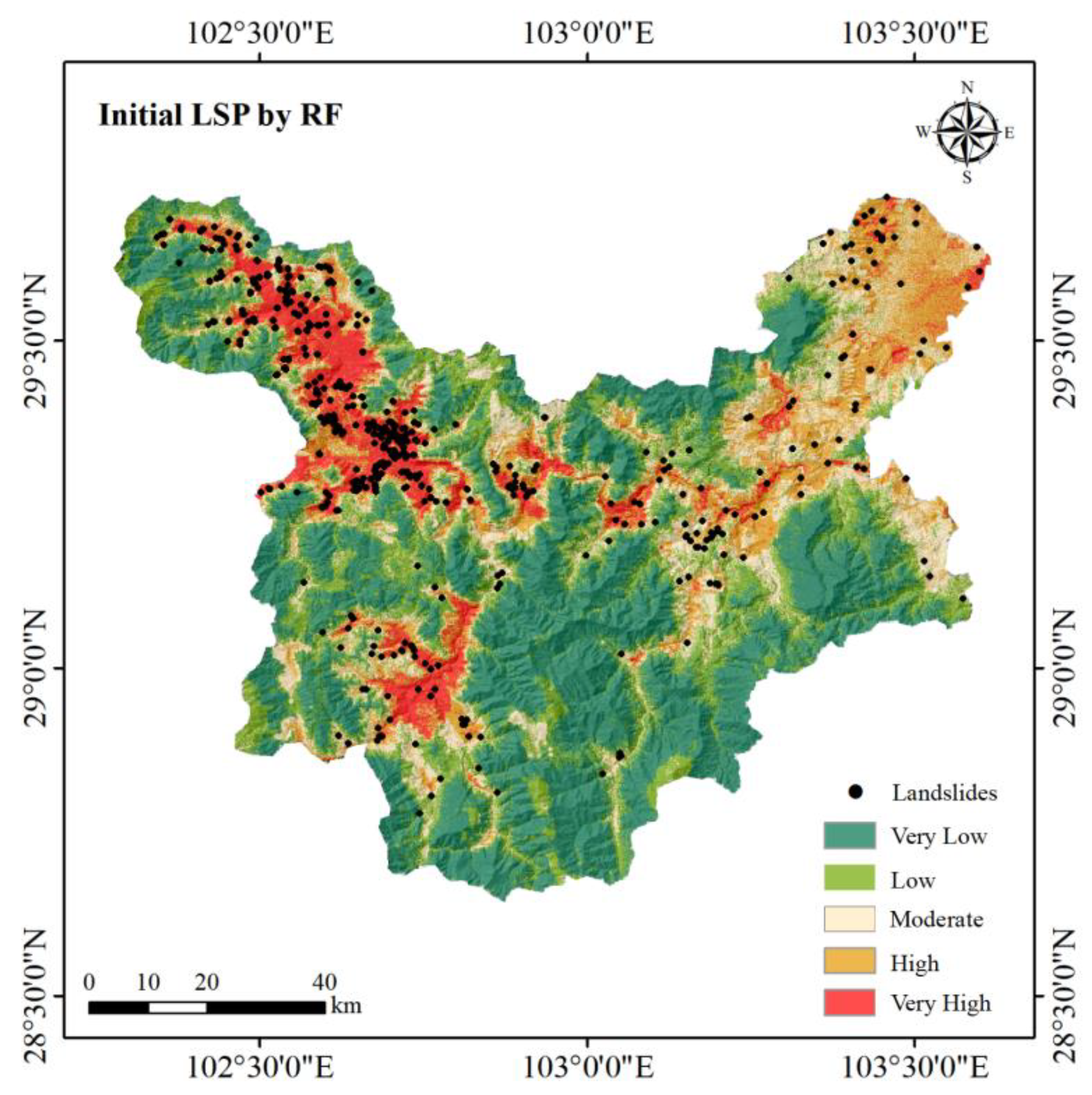
4.2. Initial LSP Results
4.2.1. Initial Landslide Susceptibility Results
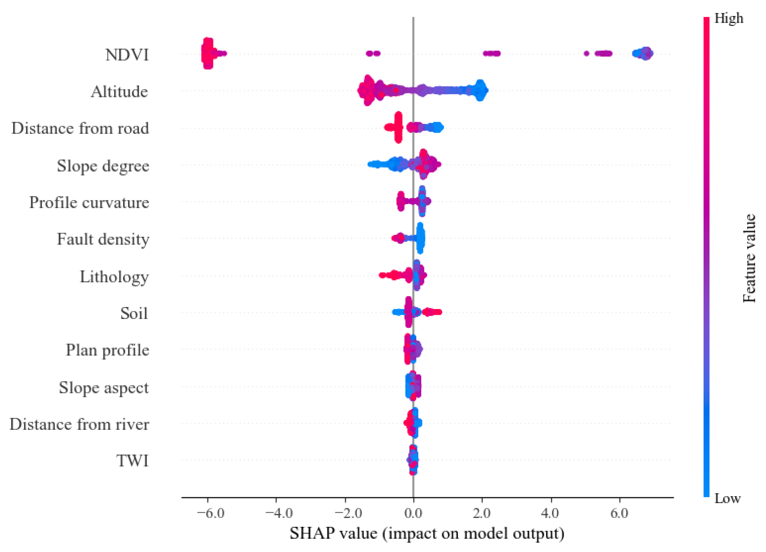
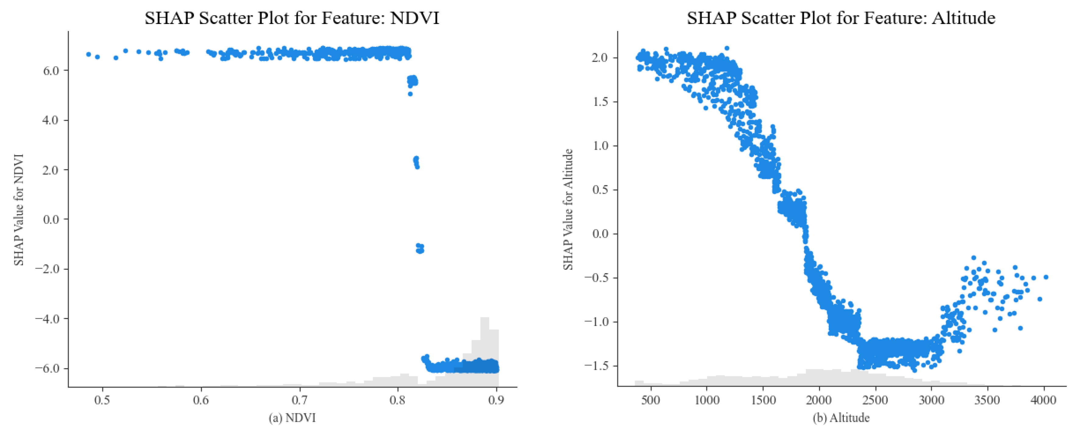
4.2.2. SHAP Value Analysis
4.3. Scenario 1
4.3.1. The Landslide Susceptibility Results for Scenario 1
4.3.2. Model Validation for Scenario 1
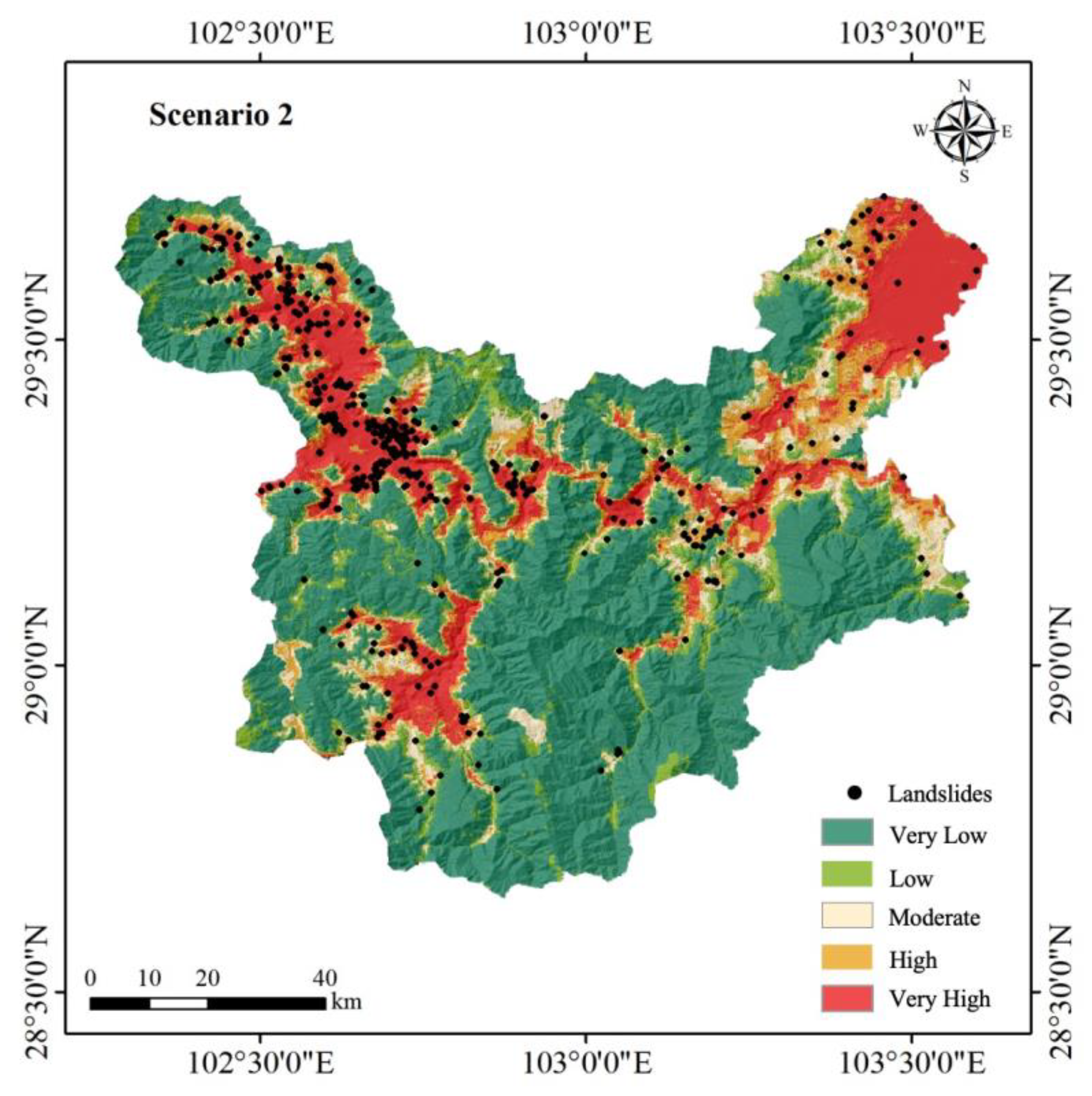
4.4. Scenario 2
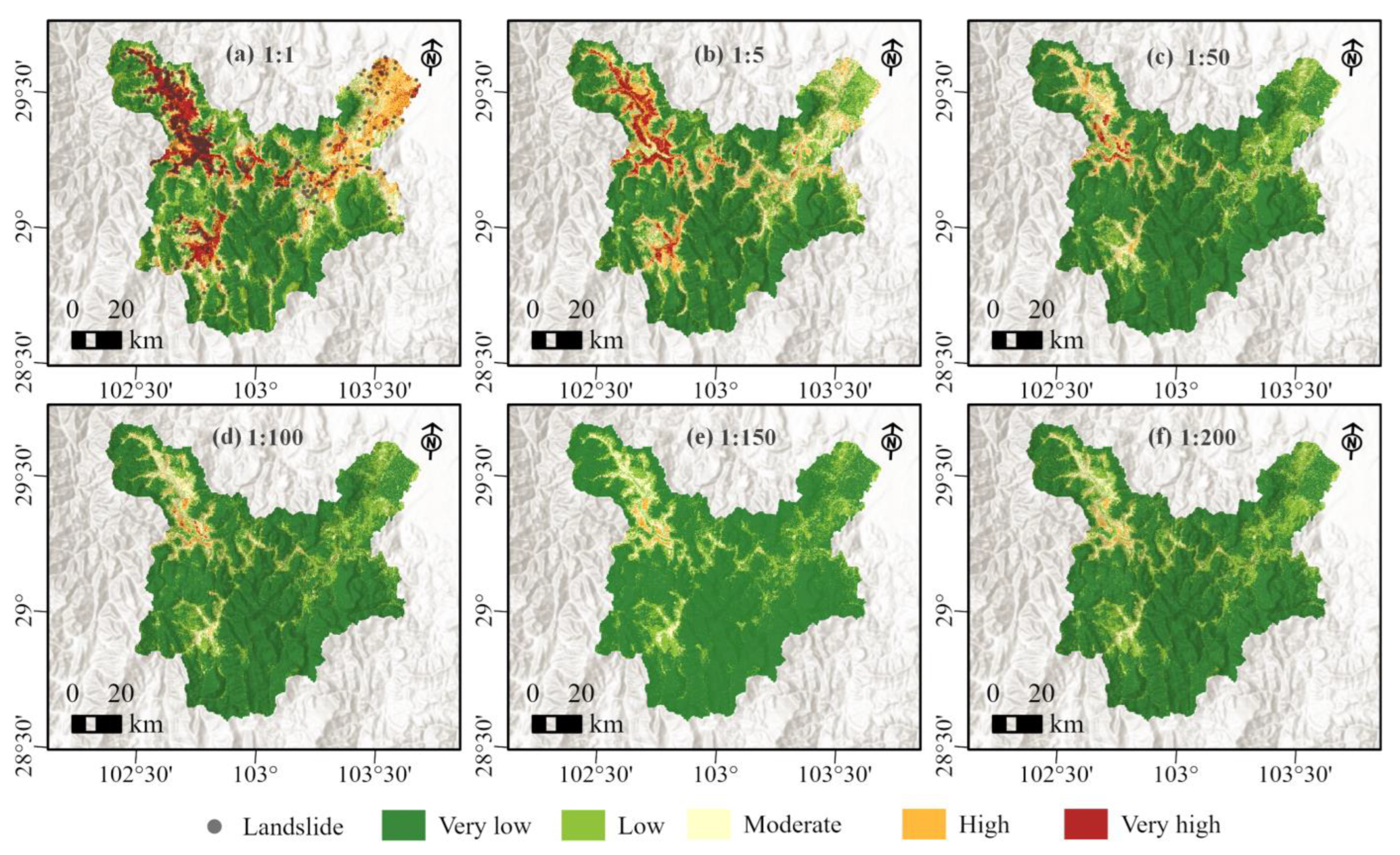
4.5. Scenario 3
5. Discussion
5.1. Frequency Ratio Analysis Results
5.2. SHAP Model Interpretation
5.3. Insights into the Three Sampling Strategies
5.4. Model Limitations and Future Perspectives
6. Conclusions
Author Contributions
Funding
Institutional Review Board Statement
Informed Consent Statement
Data Availability Statement
Conflicts of Interest
References
- Guzzetti, F.; Mondini, A.C.; Cardinali, M.; Fiorucci, F.; Santangelo, M.; Chang, K.-T. Landslide Inventory Maps: New Tools for an Old Problem. Earth-Sci. Rev. 2012, 112, 42–66. [Google Scholar] [CrossRef]
- Froude, M.J.; Petley, D.N. Global Fatal Landslide Occurrence from 2004 to 2016. Nat. Hazards Earth Syst. Sci. 2018, 18, 2161–2181. [Google Scholar] [CrossRef]
- Varnes, D.J. Landslide Types and Processes. Landslides Eng. Pract. 1958, 24, 20–47. [Google Scholar]
- Ado, M.; Amitab, K.; Maji, A.K.; Jasińska, E.; Gono, R.; Leonowicz, Z.; Jasiński, M. Landslide Susceptibility Mapping Using Machine Learning: A Literature Survey. Remote Sens. 2022, 14, 3029. [Google Scholar] [CrossRef]
- Brabb, E.E. The San Mateo County California GIS Project for Predicting the Consequences of Hazardous Geologic Processes. In Geographical Information Systems in Assessing Natural Hazards; Carrara, A., Guzzetti, F., Eds.; Advances in Natural and Technological Hazards Research; Springer: Dordrecht, The Netherlands, 1995; Volume 5, pp. 299–334. ISBN 978-90-481-4561-4. [Google Scholar]
- Corominas, J.; van Westen, C.; Frattini, P.; Cascini, L.; Malet, J.-P.; Fotopoulou, S.; Catani, F.; Van Den Eeckhaut, M.; Mavrouli, O.; Agliardi, F.; et al. Recommendations for the Quantitative Analysis of Landslide Risk. Bull. Eng. Geol. Environ. 2014, 73, 209–263. [Google Scholar] [CrossRef]
- Neuland, H. A Prediction Model of Landslips. CATENA 1976, 3, 215–230. [Google Scholar] [CrossRef]
- Aleotti, P.; Chowdhury, R. Landslide Hazard Assessment: Summary Review and New Perspectives. Bull. Eng. Geol. Environ. 1999, 58, 21–44. [Google Scholar] [CrossRef]
- Sim, A.; Ong, D.; Bachat, J. Geomorphological Approach for Assessment of Slope Stability and Landslide Hazard Mapping. In Proceedings of the 19th Southeast Asian Geotechnical Conference & 2nd AGSSEA Conference (19SEAGC & 2AGSSEA), Kuala Lumpur, Malaysia, 30 May 2016. [Google Scholar]
- Thapa, S.; Karna, A.K.; Dahal, B.K. Evaluation of Different Landslide Susceptibility Analysis Methods: A Case Study of Bagmati Rural Municipality. J. Eng. Technol. Plan. 2022, 3, 44–59. [Google Scholar] [CrossRef]
- Skempton, A.W.; Delory, F.A. Stability of Natural Slopes in London Clay. In Selected Papers on Soil Mechanics; Thomas Telford Publishing: London, UK, 1984; pp. 70–73. ISBN 978-0-7277-3982-7. [Google Scholar]
- Hao, L.; Rajaneesh, A.; van Westen, C.; Sajinkumar, K.S.; Martha, T.R.; Jaiswal, P.; McAdoo, B. Constructing a Complete Landslide Inventory Dataset for the 2018 Monsoon Disaster in Kerala, India, for Land Use Change Analysis. Earth Syst. Sci. Data 2020, 12, 2899–2918. [Google Scholar] [CrossRef]
- Carrara, A.; Cardinali, M.; Detti, R.; Guzzetti, F.; Pasqui, V.; Reichenbach, P. GIS Techniques and Statistical Models in Evaluating Landslide Hazard. Earth Surf. Process. Landf. 1991, 16, 427–445. [Google Scholar] [CrossRef]
- Huang, F.; Xiong, H.; Jiang, S.-H.; Yao, C.; Fan, X.; Catani, F.; Chang, Z.; Zhou, X.; Huang, J.; Liu, K. Modelling Landslide Susceptibility Prediction: A Review and Construction of Semi-Supervised Imbalanced Theory. Earth-Sci. Rev. 2024, 250, 104700. [Google Scholar] [CrossRef]
- Reichenbach, P.; Rossi, M.; Malamud, B.D.; Mihir, M.; Guzzetti, F. A Review of Statistically-Based Landslide Susceptibility Models. Earth-Sci. Rev. 2018, 180, 60–91. [Google Scholar] [CrossRef]
- Mitrofanov, S.A.; Semenkin, E.S. Tree Retraining in the Decision Tree Learning Algorithm. IOP Conf. Ser. Mater. Sci. Eng. 2021, 1047, 012082. [Google Scholar] [CrossRef]
- Arabameri, A.; Pal, S.C.; Rezaie, F.; Chakrabortty, R.; Saha, A.; Blaschke, T.; Di Napoli, M.; Ghorbanzadeh, O.; Ngo, P.T.T. Decision Tree Based Ensemble Machine Learning Approaches for Landslide Susceptibility Mapping. Geocarto Int. 2022, 37, 4594–4627. [Google Scholar] [CrossRef]
- Merghadi, A.; Yunus, A.P.; Dou, J.; Whiteley, J.; ThaiPham, B.; Bui, D.T.; Avtar, R.; Abderrahmane, B. Machine Learning Methods for Landslide Susceptibility Studies: A Comparative Overview of Algorithm Performance. Earth-Sci. Rev. 2020, 207, 103225. [Google Scholar] [CrossRef]
- Ma, Z.; Mei, G.; Piccialli, F. Machine Learning for Landslides Prevention: A Survey. Neural Comput. Appl. 2021, 33, 10881–10907. [Google Scholar] [CrossRef]
- Pourghasemi, H.R.; Rahmati, O. Prediction of the Landslide Susceptibility: Which Algorithm, Which Precision? CATENA 2018, 162, 177–192. [Google Scholar] [CrossRef]
- Pourghasemi, H.R.; Kornejady, A.; Kerle, N.; Shabani, F. Investigating the Effects of Different Landslide Positioning Techniques, Landslide Partitioning Approaches, and Presence-Absence Balances on Landslide Susceptibility Mapping. CATENA 2020, 187, 104364. [Google Scholar] [CrossRef]
- Zhu, A.-X.; Miao, Y.; Yang, L.; Bai, S.; Liu, J.; Hong, H. Comparison of the Presence-Only Method and Presence-Absence Method in Landslide Susceptibility Mapping. CATENA 2018, 171, 222–233. [Google Scholar] [CrossRef]
- Jiang, Y.; Wang, W.; Zou, L.; Cao, Y. Regional Landslide Susceptibility Assessment Based on Improved Semi-Supervised Clustering and Deep Learning. Acta Geotech. 2024, 19, 509–529. [Google Scholar] [CrossRef]
- Gao, H.; Fam, P.S.; Tay, L.T.; Low, H.C. Three Oversampling Methods Applied in a Comparative Landslide Spatial Research in Penang Island, Malaysia. SN Appl. Sci. 2020, 2, 1512. [Google Scholar] [CrossRef]
- Zhang, S. A Comprehensive Approach to the Observation and Prevention of Debris Flows in China. Nat. Hazards 1993, 7, 1–23. [Google Scholar] [CrossRef]
- Schicker, R.; Moon, V. Comparison of Bivariate and Multivariate Statistical Approaches in Landslide Susceptibility Mapping at a Regional Scale. Geomorphology 2012, 161–162, 40–57. [Google Scholar] [CrossRef]
- Rosser, B.; Dellow, S.; Haubrock, S.; Glassey, P. New Zealand’s National Landslide Database. Landslides 2017, 14, 1949–1959. [Google Scholar] [CrossRef]
- Huang, Y.; Zhao, L. Review on Landslide Susceptibility Mapping Using Support Vector Machines. CATENA 2018, 165, 520–529. [Google Scholar] [CrossRef]
- Haitovsky, Y. Multicollinearity in Regression Analysis: Comment. Rev. Econ. Stat. 1969, 51, 486–489. [Google Scholar] [CrossRef]
- Youssef, A.M.; Pourghasemi, H.R. Landslide Susceptibility Mapping Using Machine Learning Algorithms and Comparison of Their Performance at Abha Basin, Asir Region, Saudi Arabia. Geosci. Front. 2021, 12, 639–655. [Google Scholar] [CrossRef]
- Çellek, S. Effect of the Slope Angle and Its Classification on Landslide. Nat. Hazards Earth Syst. Sci. 2020, preprint. [Google Scholar]
- Dai, F.C.; Lee, C.F.; Li, J.; Xu, Z.W. Assessment of Landslide Susceptibility on the Natural Terrain of Lantau Island, Hong Kong. Environ. Geol. 2001, 40, 381–391. [Google Scholar] [CrossRef]
- Yilmaz, I. Landslide Susceptibility Mapping Using Frequency Ratio, Logistic Regression, Artificial Neural Networks and Their Comparison: A Case Study from Kat Landslides (Tokat—Turkey). Comput. Geosci. 2009, 35, 1125–1138. [Google Scholar] [CrossRef]
- Sørensen, R.; Zinko, U.; Seibert, J. On the Calculation of the Topographic Wetness Index: Evaluation of Different Methods Based on Field Observations. Hydrol. Earth Syst. Sci. 2006, 10, 101–112. [Google Scholar] [CrossRef]
- Agboola, G.; Beni, L.H.; Elbayoumi, T.; Thompson, G. Optimizing Landslide Susceptibility Mapping Using Machine Learning and Geospatial Techniques. Ecol. Inform. 2024, 81, 102583. [Google Scholar] [CrossRef]
- Chen, W.; Li, Y. GIS-Based Evaluation of Landslide Susceptibility Using Hybrid Computational Intelligence Models. CATENA 2020, 195, 104777. [Google Scholar] [CrossRef]
- Hall, F.G.; Townshend, J.R.; Engman, E.T. Status of Remote Sensing Algorithms for Estimation of Land Surface State Parameters. Remote Sens. Environ. 1995, 51, 138–156. [Google Scholar] [CrossRef]
- Yan, G.; Liang, S.; Gui, X.; Xie, Y.; Zhao, H. Optimizing Landslide Susceptibility Mapping in the Kongtong District, NW China: Comparing the Subdivision Criteria of Factors. Geocarto Int. 2019, 34, 1408–1426. [Google Scholar] [CrossRef]
- Brenning, A.; Schwinn, M.; Ruiz-Páez, A.P.; Muenchow, J. Landslide Susceptibility near Highways Is Increased by 1 Order of Magnitude in the Andes of Southern Ecuador, Loja Province. Nat. Hazards Earth Syst. Sci. 2015, 15, 45–57. [Google Scholar] [CrossRef]
- Ilinca, V.; Şandric, I.; Jurchescu, M.; Chiţu, Z. Identifying the Role of Structural and Lithological Control of Landslides Using TOBIA and Weight of Evidence: Case Studies from Romania. Landslides 2022, 19, 2117–2134. [Google Scholar] [CrossRef]
- Hungr, O.; Leroueil, S.; Picarelli, L. The Varnes Classification of Landslide Types, an Update. Landslides 2014, 11, 167–194. [Google Scholar] [CrossRef]
- Aditian, A.; Kubota, T.; Shinohara, Y. Comparison of GIS-Based Landslide Susceptibility Models Using Frequency Ratio, Logistic Regression, and Artificial Neural Network in a Tertiary Region of Ambon, Indonesia. Geomorphology 2018, 318, 101–111. [Google Scholar] [CrossRef]
- Pourghasemi, H.R.; Teimoori Yansari, Z.; Panagos, P.; Pradhan, B. Analysis and Evaluation of Landslide Susceptibility: A Review on Articles Published during 2005–2016 (Periods of 2005–2012 and 2013–2016). Arab. J. Geosci. 2018, 11, 193. [Google Scholar] [CrossRef]
- Lundberg, S.M.; Lee, S.-I. A Unified Approach to Interpreting Model Predictions. In Proceedings of the 31st International Conference on Neural Information Processing Systems, Long Beach, CA, USA, 4–9 December 2017; Curran Associates, Inc.: Red Hook, NY, USA, 2017; Volume 30. [Google Scholar]
- Zhang, J.; Ma, X.; Zhang, J.; Sun, D.; Zhou, X.; Mi, C.; Wen, H. Insights into Geospatial Heterogeneity of Landslide Susceptibility Based on the SHAP-XGBoost Model. J. Environ. Manag. 2023, 332, 117357. [Google Scholar] [CrossRef]
- Meng, Y.; Yang, N.; Qian, Z.; Zhang, G. What Makes an Online Review More Helpful: An Interpretation Framework Using XGBoost and SHAP Values. J. Theor. Appl. Electron. Commer. Res. 2021, 16, 466–490. [Google Scholar] [CrossRef]
- Yang, B.; Lu, H.; Ran, Y. Advancing Non-Alcoholic Fatty Liver Disease Prediction: A Comprehensive Machine Learning Approach Integrating SHAP Interpretability and Multi-Cohort Validation. Front. Endocrinol. 2024, 15, 1450317. [Google Scholar] [CrossRef] [PubMed]
- Pearce, J.; Ferrier, S. Evaluating the Predictive Performance of Habitat Models Developed Using Logistic Regression. Ecol. Model. 2000, 133, 225–245. [Google Scholar] [CrossRef]
- Aguirre-Gutiérrez, J.; Carvalheiro, L.G.; Polce, C.; van Loon, E.E.; Raes, N.; Reemer, M.; Biesmeijer, J.C. Fit-for-Purpose: Species Distribution Model Performance Depends on Evaluation Criteria—Dutch Hoverflies as a Case Study. PLoS ONE 2013, 8, e63708. [Google Scholar] [CrossRef] [PubMed]
- Austin, M. Species Distribution Models and Ecological Theory: A Critical Assessment and Some Possible New Approaches. Ecol. Model. 2007, 200, 1–19. [Google Scholar] [CrossRef]
- Elith, J.H.; Graham, C.P.H.; Anderson, R.P.; Dudík, M.; Ferrier, S.; Guisan, A.; Hijmans, R.J.; Huettmann, F.; Leathwick, J.R.; Lehmann, A.; et al. Novel Methods Improve Prediction of Species’ Distributions from Occurrence Data. Ecography 2006, 29, 129–151. [Google Scholar] [CrossRef]
- Guzzetti, F.; Carrara, A.; Cardinali, M.; Reichenbach, P. Landslide Hazard Evaluation: A Review of Current Techniques and Their Application in a Multi-Scale Study, Central Italy. Geomorphology 1999, 31, 181–216. [Google Scholar] [CrossRef]
- Lee, S.; Sambath, T. Landslide Susceptibility Mapping in the Damrei Romel Area, Cambodia Using Frequency Ratio and Logistic Regression Models. Environ. Geol. 2006, 50, 847–855. [Google Scholar] [CrossRef]
- Gómez-Ramírez, J.; Ávila-Villanueva, M.; Fernández-Blázquez, M.Á. Selecting the Most Important Self-Assessed Features for Predicting Conversion to Mild Cognitive Impairment with Random Forest and Permutation-Based Methods. Sci. Rep. 2020, 10, 20630. [Google Scholar] [CrossRef] [PubMed]
- Bradley, A.P. The Use of the Area under the ROC Curve in the Evaluation of Machine Learning Algorithms. Pattern Recognit. 1997, 30, 1145–1159. [Google Scholar] [CrossRef]
- Wang, Y.; Song, Q.; Du, Y.; Wang, J.; Zhou, J.; Du, Z.; Li, T. A Random Forest Model to Predict Heatstroke Occurrence for Heatwave in China. Sci. Total Environ. 2019, 650, 3048–3053. [Google Scholar] [CrossRef] [PubMed]
- Murgia, I.; Giadrossich, F.; Mao, Z.; Cohen, D.; Capra, G.F.; Schwarz, M. Modeling Shallow Landslides and Root Reinforcement: A Review. Ecol. Eng. 2022, 181, 106671. [Google Scholar] [CrossRef]
- Murgia, I.; Giadrossich, F.; Niccolini, M.; Preti, F.; Giambastiani, Y.; Capra, G.F.; Cohen, D. Using SlideforMAP and SOSlope to Identify Susceptible Areas to Shallow Landslides in the Foreste Casentinesi National Park (Tuscany, Italy). In Proceedings of the EGU General Assembly 2021, Online, 19–30 April 2021; EGU21-14454. [Google Scholar] [CrossRef]
- Marzini, L.; D’Addario, E.; Papasidero, M.P.; Chianucci, F.; Disperati, L. Influence of Root Reinforcement on Shallow Landslide Distribution: A Case Study in Garfagnana (Northern Tuscany, Italy). Geosciences 2023, 13, 326. [Google Scholar] [CrossRef]
- Ribeiro, M.T.; Singh, S.; Guestrin, C. “Why Should I Trust You?”: Explaining the Predictions of Any Classifier. In Proceedings of the 22nd ACM SIGKDD International Conference on Knowledge Discovery and Data Mining, San Francisco, CA, USA, 13–17 August 2016; Association for Computing Machinery: New York, NY, USA, 2016; pp. 1135–1144. [Google Scholar]


| Category | LCFs | Type | Scale/Resolution | Source | Min. | Max. |
|---|---|---|---|---|---|---|
| Topographic factors | Altitude | Raster | 30 m | DEM | 363 | 4242 |
| Slope degree | Raster | 30 m | DEM | 0 | 79.54 | |
| Slope aspect | Raster | 30 m | DEM | — | — | |
| Plan Curvature | Raster | 30 m | DEM | −20.45 | 26.18 | |
| Profile curvature | Raster | 30 m | DEM | −22.21 | 20.09 | |
| TWI | Raster | 30 m | DEM | 1.66 | 30.10 | |
| Environmental factors | NDVI | Raster | 30 m | Landsat 8 satellite images | 0.32 | 0.90 |
| soil types | Vector | 1:1,000,000 | National Cryosphere Desert Data Center. (http://www.ncdc.ac.cn, accessed on June 2024) | — | — | |
| Distance from rivers | Vector | 1:250,000 | National Earth System Science Data Center, National Science & Technology Infrastructure of China (http://www.geodata.cn, accessed on June 2024) | 0 | — | |
| Distance from roads | Vector | 1:250,000 | National Earth System Science Data Center, National Science & Technology Infrastructure of China (http://www.geodata.cn, accessed on June 2024) | 0 | — | |
| Geological factors | Lithology | Vector | 1:1,000,000 | ISRIC (https://data.isric.org/, accessed on June 2024) | — | — |
| Fault density | Vector | 1:2,500,000 | Data Sharing Infrastructure of Seismic Active Fault Survey Data Center (https://www.activefault-datacenter.cn, accessed on June 2024) | 0 | 0.40 |
| LCFs | Class | Area Count | Landslides | Percent of Area (E) | Percent of Landslide (F) | FR = F/E | RF (%) | Max |
|---|---|---|---|---|---|---|---|---|
| Altitude | 2820–4242 | 126,099 | 154 | 15% | 26% | 1.79 | 37% | 2.37 |
| 2196–2820 | 199,557 | 322 | 23% | 55% | 2.37 | 49% | ||
| 1638–2196 | 235,332 | 105 | 27% | 18% | 0.66 | 13% | ||
| 1050–1638 | 210,888 | 8 | 24% | 1% | 0.06 | 1% | ||
| 363–1050 | 93,578 | 0 | 11% | 0% | 0.00 | 0% | ||
| Slope degree | 42.23–79.5 | 147,764 | 142 | 17% | 24% | 1.41 | 30% | 1.64 |
| 31.9–42.23 | 210,399 | 236 | 24% | 40% | 1.64 | 35% | ||
| 22.5–31.9 | 223,029 | 143 | 26% | 24% | 0.94 | 20% | ||
| 12.7–22.5 | 193,543 | 45 | 22% | 8% | 0.34 | 7% | ||
| 0–12.7 | 88,984 | 23 | 10% | 4% | 0.38 | 8% | ||
| Slope aspect | N | 97,782 | 49 | 11% | 8% | 0.73 | 9% | 1.29 |
| NE | 113,375 | 58 | 13% | 10% | 0.75 | 9% | ||
| E | 120,747 | 83 | 14% | 14% | 1.00 | 13% | ||
| ES | 107,297 | 83 | 12% | 14% | 1.13 | 14% | ||
| S | 94,668 | 78 | 11% | 13% | 1.20 | 15% | ||
| WS | 100,338 | 89 | 12% | 15% | 1.29 | 16% | ||
| W | 115,858 | 88 | 13% | 15% | 1.11 | 14% | ||
| WN | 108,574 | 60 | 13% | 10% | 0.81 | 10% | ||
| Plan curvature | −20.4–2.05 | 29,969 | 11 | 3% | 2% | 0.54 | 14% | 1.18 |
| −2.05–0.78 | 132,209 | 66 | 15% | 11% | 0.73 | 19% | ||
| −0.78–0.32 | 402,999 | 325 | 47% | 55% | 1.18 | 30% | ||
| 0.32–1.77 | 255,768 | 174 | 30% | 30% | 1.00 | 26% | ||
| 1.77–26.18 | 44,509 | 13 | 5% | 2% | 0.43 | 11% | ||
| Profile curvature | 1.75–20.09 | 26,664 | 3 | 3% | 1% | 0.17 | 5% | 1.29 |
| 0.26–1.75 | 131,915 | 65 | 15% | 11% | 0.72 | 21% | ||
| −0.89–0.25 | 371,154 | 325 | 43% | 55% | 1.29 | 38% | ||
| −2.55–0.89 | 273,141 | 174 | 32% | 30% | 0.94 | 27% | ||
| −22.21–2.55 | 62,580 | 13 | 7% | 2% | 0.31 | 9% | ||
| TWI | 1.66–4.66 | 377,624 | 212 | 44% | 36% | 0.82 | 14% | 1.52 |
| 4.66–6.54 | 297,552 | 216 | 34% | 37% | 1.06 | 18% | ||
| 6.54–9.33 | 130,604 | 103 | 15% | 17% | 1.16 | 20% | ||
| 9.33–14.44 | 40,507 | 42 | 5% | 7% | 1.52 | 26% | ||
| 14.44–30.10 | 17,432 | 16 | 2% | 3% | 1.35 | 23% | ||
| NDVI | 0.32–0.64 | 10,567 | 27 | 1% | 5% | 3.70 | 31% | 3.70 |
| 0.64–0.75 | 37,688 | 84 | 4% | 14% | 3.23 | 27% | ||
| 0.75–0.81 | 89,102 | 221 | 10% | 38% | 3.59 | 30% | ||
| 0.81–0.86 | 215,742 | 190 | 25% | 32% | 1.28 | 11% | ||
| 0.86–0.9 | 500,027 | 67 | 59% | 11% | 0.19 | 2% | ||
| Soil types | Lixisols | 95,685.81 | 145 | 11% | 25% | 2.24 | 21% | 2.24 |
| Regosols | 104,384.52 | 133 | 12% | 23% | 1.88 | 18% | ||
| Anthrosols | 43,493.55 | 56 | 5% | 8% | 1.56 | 15% | ||
| Luvisols | 43,4935.5 | 35 | 50% | 6% | 0.12 | 1% | ||
| Cambisols | 69,589.68 | 35 | 8% | 6% | 0.75 | 7% | ||
| Distance from river | 0–500 | 169,088 | 208 | 19% | 35% | 1.82 | 33% | 1.82 |
| 500–1000 | 147,156 | 107 | 17% | 18% | 1.07 | 20% | ||
| 1000–1500 | 134,586 | 94 | 15% | 16% | 1.03 | 19% | ||
| 1500–2000 | 114,475 | 80 | 13% | 14% | 1.03 | 19% | ||
| >2000 | 304,566 | 100 | 35% | 17% | 0.48 | 9% | ||
| Distance from road | 0–500 | 133,635 | 212 | 15% | 36% | 2.34 | 35% | 2.34 |
| 500–1000 | 100,139 | 103 | 12% | 17% | 1.52 | 23% | ||
| 1000–1500 | 87,300 | 64 | 10% | 11% | 1.08 | 16% | ||
| 1500–2000 | 76,050 | 63 | 9% | 11% | 1.22 | 18% | ||
| >2000 | 472,747 | 147 | 54% | 25% | 0.46 | 7% | ||
| Fault density | 0–0.037 | 443,076 | 343 | 51% | 58% | 1.14 | 26% | 1.14 |
| 0.037–0.105 | 129,035 | 84 | 15% | 14% | 0.96 | 22% | ||
| 0.105–0.170 | 201,592 | 115 | 23% | 20% | 0.84 | 19% | ||
| 0.170–0.25 | 68,716 | 37 | 8% | 6% | 0.79 | 18% | ||
| 0.25–0.401 | 23,009 | 10 | 3% | 2% | 0.64 | 15% |
| Landslide/Non-Landslide | Landslide Slope Units | Non-Landslide Slope Units | Total Number of Landslide and Non-Landslide Slope Units | Training Set (70%) | Test Set (30%) |
|---|---|---|---|---|---|
| 1:1 | 589 | 589 | 1178 | 824 | 353 |
| LCFs | Class | Area Count | Landslides | % of Area (E) | % of Landslide (F) | FR = F/E |
|---|---|---|---|---|---|---|
| Altitude | Very Low | 326,157 | 3 | 38% | 1% | 0.01 |
| Low | 197,596 | 11 | 23% | 2% | 0.08 | |
| Moderate | 131,483 | 38 | 15% | 6% | 0.42 | |
| High | 119,645 | 90 | 14% | 15% | 1.09 | |
| Very high | 77,189 | 445 | 9% | 76% | 8.37 |
| Landslide/Non-Landslide | Landslide Slope Units | Non-Landslide Slope Units | Total Number of Landslide and Non-Landslide Slope Units | Training Set (70%) | Test Set (30%) |
|---|---|---|---|---|---|
| 1:1 | 589 | 589 | 1178 | 824 | 353 |
| 1:5 | 589 | 2945 | 3534 | 2474 | 1061 |
| 1:50 | 589 | 29,450 | 30,039 | 21,027 | 9012 |
| 1:100 | 589 | 58,900 | 59,489 | 41,642 | 17,847 |
| 1:150 | 589 | 88,350 | 88,939 | 62,257 | 26,682 |
| 1:200 | 589 | 117,800 | 118,389 | 82,872 | 35,517 |
Disclaimer/Publisher’s Note: The statements, opinions and data contained in all publications are solely those of the individual author(s) and contributor(s) and not of MDPI and/or the editor(s). MDPI and/or the editor(s) disclaim responsibility for any injury to people or property resulting from any ideas, methods, instructions or products referred to in the content. |
© 2025 by the authors. Licensee MDPI, Basel, Switzerland. This article is an open access article distributed under the terms and conditions of the Creative Commons Attribution (CC BY) license (https://creativecommons.org/licenses/by/4.0/).
Share and Cite
Li, M.; Tian, H. Insights from Optimized Non-Landslide Sampling and SHAP Explainability for Landslide Susceptibility Prediction. Appl. Sci. 2025, 15, 1163. https://doi.org/10.3390/app15031163
Li M, Tian H. Insights from Optimized Non-Landslide Sampling and SHAP Explainability for Landslide Susceptibility Prediction. Applied Sciences. 2025; 15(3):1163. https://doi.org/10.3390/app15031163
Chicago/Turabian StyleLi, Mengyuan, and Hongling Tian. 2025. "Insights from Optimized Non-Landslide Sampling and SHAP Explainability for Landslide Susceptibility Prediction" Applied Sciences 15, no. 3: 1163. https://doi.org/10.3390/app15031163
APA StyleLi, M., & Tian, H. (2025). Insights from Optimized Non-Landslide Sampling and SHAP Explainability for Landslide Susceptibility Prediction. Applied Sciences, 15(3), 1163. https://doi.org/10.3390/app15031163