Wind Reference Year: A New Approach

Abstract

The representativeness of long-term wind data at a site remains a challenge, as it is essential for resource analysis, production adjustment in operating plants, and the simulation of hybridised plants. A representative one-year hourly time series, known as a Wind Reference Year (WRY), is required, yet the availability of long-term real data is rare, making the estimation of WRY from reanalysis data and shorter measurement campaigns a common approach. In this study, Gaussian Mixture Copula Models (GMCM) and five regression models were applied and compared. The GMCM was trained using 15 years of reanalysis data to generate simulations, and subsequently, regression-based Measure–Correlate–Predict (MCP) methods were applied to adapt the simulated reference year to site-specific conditions. Finally, the Hungarian algorithm was used to reorder the simulated data series, aligning it with a typical wind pattern and producing the WRY dataset. The results were validated against 15 years of real measurements and benchmarked against a heuristic method based on long-term similarity of main wind parameters and the commercial tool Windographer. The findings demonstrate the potential of the proposed method, showing improvements over existing techniques and providing a robust approach to constructing representative WRY datasets.

1. Introduction

In wind energy projects, due diligence in the pre-construction phase typically requires an expensive data collection campaign lasting at least one full year, followed by long-term extrapolation over the project lifetime. In the current energy context—with an urgent need to reduce fossil-fuel dependence via renewables—hybrid projects that combine several resources are expected to expand rapidly, providing greater stability in power generation. The benefits and market opportunities of hybrid systems and renewables are discussed in [1,2].

A central challenge when estimating expected energy production for a given scenario is the accurate characterisation of the site’s typical wind-energy content. Recent overviews of energy-production prediction bias and loss accounting highlight that long-term resource characterisation and uncertainty quantification are now central elements of modern wind project due diligence [3], underscoring the need for representative datasets that reflect multi-year climatic variability. Most specialised simulation tools rely on reference years to estimate production at a site. Furthermore, recent analyses of long-term resource uncertainty show that variability in the underlying wind resource can propagate into significant AEP deviations in real projects [4], reinforcing the need for representative reference-year datasets. For compatibility with such tools (e.g., WAsP, HOMER), a reference year of the relevant resource (wind, solar, etc.) is required. This dataset must capture long-term climatic conditions (typically 15–20 years) while condensing them into a single “typical” year of 8760 hourly values.

The concept of a typical meteorological year has been widely studied in building-energy performance [5,6] and solar-resource assessment. Overviews and comparisons of algorithms can be found in [7,8]. More recently, ref. [9] constructed a global TMY database directly from ERA5, confirming the feasibility of reanalysis-based typical years for building- and renewable-energy applications. Similarly, in the urban context, ref. [10] used ERA5 in combination with an urban canopy model to generate urban typical meteorological year (uTMY) datasets for building-energy simulations, further illustrating the flexibility of reanalysis-based typical years across different applications. One of the most-used methods is the Sandia approach, which selects 12 typical months from a long-term dataset and concatenates them into a representative year [11]. Updated versions were later developed at NREL [12,13]. Further developments include the modification of Sandia’s method to generate typical years at different time resolutions [14]. However, classical TMY/WRY approaches were originally developed for building- and solar-energy applications and were not designed to preserve multi-site dependence, long-term climatic variability, or modern uncertainty requirements. Recent studies have shown that these aspects are critical for contemporary wind-resource assessment [3,4].

In the wind industry, however, there is no universally accepted methodology for generating a Wind Reference Year (WRY). As noted in [15], a method based on the Finkelstein–Schafer statistic has been proposed and applied to a real case using reanalysis data. Since multi-year measurements are seldom available, reliance on long-term reanalysis products (e.g., ERA5 [16]) has increased. Reanalysis nodes exhibit substantial uncertainties: they provide grid-averaged hourly values that require adaptation to the specific site. Recent validation studies [17] show that ERA5 can provide reliable long-term wind resources and AEP estimates at flat and offshore sites, but performance degrades in complex terrain and coastal regions, highlighting the need for local adaptation methods such as MCP. This site-adaptation process, common in climate and meteorology, adjusts long-term modelled variables by comparison with observations. For example, refs. [18,19] explored bias-correction techniques based on quantile mapping. A recent critical review [20] synthesises the main sources of uncertainty across 15 global and regional reanalysis products at more than 300 sites worldwide, underlining that spatial biases remain a key limitation for long-term wind resource assessment and reinforcing the need for local adaptation procedures such as MCP.

Most often, Measure–Correlate–Predict (MCP) is used to obtain representative long-term series: short-term site measurements are related to long-term references and corrected accordingly. In [21,22], the bin method is compared to linear regression, and ref. [23] provides an extensive review of MCP methods since the 1940s, highlighting limitations and uncertainties. The MEASNET guide [24] recommends combining site data (e.g., met-mast measurements) with concurrent long-term reference series, whether reanalysis or off-site measurements. More recent developments continue to demonstrate the relevance of advanced MCP formulations for long-term wind-resource assessment. For example, ref. [25] applied an enhanced MCP framework to transfer wind speeds from MERRA2 reanalysis to turbine hub heights, achieving substantial improvements in long-term representativeness. These results highlight the importance of robust MCP-based site-adaptation procedures when reanalysis data exhibit spatial or height-related discrepancies.

To complement these developments and situate our work within the broader landscape of modern wind-energy modelling, several hybrid learning–observer approaches have also been explored to address uncertainty, noise, and stochastic variability. For instance, ref. [26] proposed ANFIS-based interval observers for robust fault detection in wind turbines, while ref. [27] developed MANFIS architectures combined with zonotopic observers to enhance resilience against measurement disturbances and model inaccuracies. Although these methods focus primarily on short-term operational dynamics rather than long-term climatological representativeness, they illustrate the increasing adoption of advanced data-driven and hybrid estimation techniques in wind-energy applications.

A notable example of reference-year construction is PVGIS (Photovoltaic Geographical Information System) [28], which provides typical meteorological years for nine climatic variables by selecting the most representative months over a long-term period. The methodology, described in [29] and based on ISO 15927-4 [30], relies on the Finkelstein–Schafer statistic, with primary variables (irradiance, temperature, humidity) and secondary variables (such as wind speed). Although PVGIS targets solar energy and building applications, it also reports wind speed at 10 m without site adaptation. Commercial tools such as Windographer [31] use Markov chains to generate representative years and include an MCP module for long-term extrapolation. Combining MCP-based site adaptation with a Markov chain generator enables a site-specific WRY.

In this work, machine-learning models are applied to capture long-term wind behaviour from 15 to 20 years of reanalysis. Specifically, Gaussian Mixture Copula Models (GMCMs) are used [32]. Prior studies have leveraged GMCMs to augment machine-learning inputs with synthetic series [33]. Here, synthetic data are generated to emulate long-term behaviour in an 8760-h dataset. Copula-based modelling has also seen increasing use in power-system applications, where it enables the generation of spatiotemporal wind-power scenarios together with explicit treatment of forecast errors [34]. While such approaches focus on short-term operational uncertainty, the GMCM-based WRY developed in this work addresses a complementary problem: the long-term climatological representation of wind-resource variability.

Alternative approaches to impose temporal dependence on synthetic resource series include dependent-bootstrap schemes and sequence-assembly methods. In wind and solar applications, moving-block bootstrap techniques are widely used to reconstruct short-term persistence by resampling contiguous blocks of historical data [35,36,37]. A second family of techniques relies on rank-based reordering, most notably the Schaake Shuffle and its more recent variants, which restore temporal and spatial consistency by imposing the rank structure of historical observations [38,39,40]. While these methods are effective for generating coherent time series, they either replicate historical blocks or impose dependence indirectly through rank structure. In contrast, assignment-based approaches such as that introduced by Naimo [41] provide a deterministic and distribution-preserving way to enforce persistence. Building on this line of work, the present study applies the Hungarian algorithm to introduce realistic temporal structure without altering the marginal or multivariate characteristics learned from long-term reanalysis.

The proposed pipeline proceeds in three steps. First, copulas capture inter-variable dependencies and generate synthetic data consistent with the training period (GMCM). Second, the simulated series are adapted to site conditions via multiple regression models following the MCP framework, using one year of on-site measurements and long-term reanalysis. Finally, the simulated and site-adapted data are rearranged to preserve wind persistence and to ensure a consistent intra-annual wind pattern; to this end, the Hungarian algorithm is applied [41].

2. Case and Data Definition

To develop the Wind Reference Year (WRY) methodology and to verify results, both reanalysis and on-site measurements were considered (Table 1). The datasets used in this work are as follows:

• ERA5 reanalysis data. Fifteen years (2006–2020) from three grid nodes near the study site were used. Hourly series were retrieved via the ECMWF Climate Data Store API [16]. These data provide the long-term reference to learn the climatological behaviour and to feed the WRY modelling.
• Operational data (on-site measurements). Wind-speed measurements from a wind farm in Spain spanning fifteen years (2006–2020) at a 10 min sampling interval. These data serve two purposes: (i) long-term validation of the WRY-based energy estimates against the multi-year record and (ii) training MCP regression models with a one-year concurrent subset to transpose reanalysis-based simulations to site conditions (emulating a typical project scenario with limited campaign data). The representative power curve derived from the site’s turbine (pitch-regulated turbine, 1 MW rated power) is used to convert wind speed to energy for comparison.

Table 1. Datasets used in this study.

Dataset	Years	Resolution	Nodes/Site	Role	Notes
ERA5 reanalysis	2006–2020	Hourly	3 nodes (near site)	Long-term reference; WRY modelling	Retrieved via ECMWF CDS API.
Operational (site)	2006–2020	10 min	Wind farm (Spain)	MCP training (1 yr) and long-term validation	Representative power curve: pitch-regulated, 1 MW.

Table 1. Datasets used in this study.

Dataset	Years	Resolution	Nodes/Site	Role	Notes
ERA5 reanalysis	2006–2020	Hourly	3 nodes (near site)	Long-term reference; WRY modelling	Retrieved via ECMWF CDS API.
Operational (site)	2006–2020	10 min	Wind farm (Spain)	MCP training (1 yr) and long-term validation	Representative power curve: pitch-regulated, 1 MW.

3. Methodology

3.1. Flowchart of the WRY Generation Process

This work proposes the use of the Gaussian Mixture Copula Model (GMCM) to construct a Wind Reference Year (WRY) from long-term reanalysis and a short on-site campaign. Reanalysis series are first adjusted to hub height using a power-law profile (nodes at 10 m to 55 m) with shear coefficient $\alpha =0.14$ [42]. Once the WRY is obtained, wind speed is mapped to power using the representative power curve derived from the site’s turbine (pitch-regulated, 1 MW), and the resulting Annual Energy Production (AEP) is compared against the average AEP from 15 years of operational data.

3.1.1. Proposed Method (GMCM)

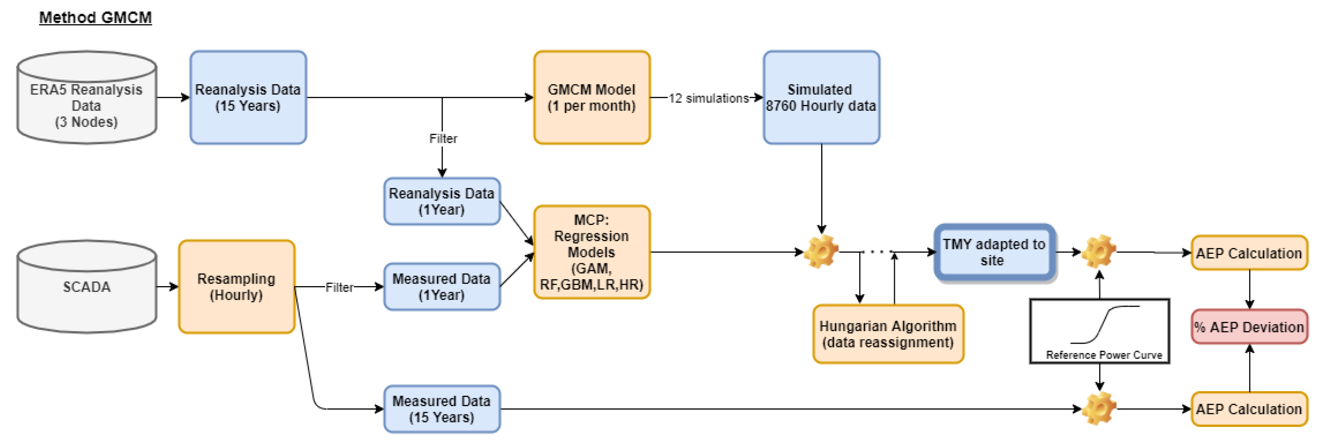
The GMCM-based workflow (Figure 1) learns the long-term joint behaviour of the reanalysis variables and generates synthetic months that reproduce those patterns. The copula component captures the joint dependence of the variables across the three ERA5 nodes, so sampling from the Gaussian Mixture Copula Model (GMCM) yields hourly series whose key statistics and inter-variable relationships match the training period [32]. The stages are as follows:

(i)

Long-term learning. GMCMs [32] are trained on 15 years of ERA5 data from the three nearest grid nodes to the site, capturing their combined information. Data are split by calendar month, and 12 monthly models are obtained, with each model fitted to the corresponding 15-month subset (e.g., 15 Januaries, 15 Februaries, etc.). This design preserves seasonality while learning long-term behaviour and the dependence structure.

(ii)

Monthly simulation and concatenation. For each month, the trained GMCM generates a synthetic hourly series whose distribution reflects the 15-year training months. The 12 synthetic months are concatenated to form an 8760 h WRY at the reanalysis-node level.

(iii)

Site adaptation (MCP). The synthetic WRY is adapted to site conditions using regression-based MCP with one year of concurrent measurements and reanalysis. The following models are evaluated: Generalised Additive Model (GAM), Gradient Boosting Regressor (GBR), Random Forest (RF), Linear Regression (LR), and Huber Regression (HR).

(iv)

Temporal reordering. Because GMCM outputs preserve distributional properties but not temporal order, the simulated and site-adapted series are rearranged to preserve wind persistence and ensure a consistent wind pattern. For this purpose, the Hungarian algorithm is applied [41].

(v)

Energy assessment. The site-adapted WRY is converted to power using the representative power curve and yielding the AEP estimate, which is then compared with the 15-year operational benchmark.

Figure 1. Diagram of the proposed GMCM-based WRY calculation process.

Figure 1. Diagram of the proposed GMCM-based WRY calculation process.

3.1.2. Baselines for Comparison

To contextualise performance, two widely used alternatives are implemented under the same pre-/post-processing (power-law adjustment and power-curve mapping):

(i) 

Heuristic month selection: Following the guidelines of ISO 15927-4 [30], for each calendar month, the most representative month in the historical data is selected, and the 12 months are concatenated into a WRY. To reduce subjectivity, similarity is quantified by the Euclidean distance in the space defined by the monthly mean wind speed and Weibull shape/scale. The assembled WRY is then adapted to the site via MCP, using the one-year concurrent measurements, and its AEP is compared to the AEP derived from the multi-year operational data.

(ii) 

Windographer workflow. Windographer is a commercial tool that provides a workflow for constructing a WRY. First, the MCP module adapts the 15-year reanalysis record to the site using one year of measured wind speed. The Representative Year Window tool (Markov-chain-based) is then applied to generate the WRY. The resulting AEP is compared with that derived from the multi-year operational data.

Finally, results are reported as AEP deviations relative to the 15-year average from operational data, enabling a direct comparison between the proposed GMCM pipeline and the two baselines.

3.2. Modelling WRY

A key design choice in the proposed approach is to jointly model the three ERA5 nodes nearest to the site. Treating these nodes as a multivariate system allows for the model to learn not only each node’s marginal behaviour but also the cross-node structure that reflects local and regional dynamics (e.g., prevailing synoptic regimes). Copula-based modelling is well suited to this purpose because it explicitly captures dependence among variables [43]; in our case, the Gaussian Mixture Copula Model (GMCM) provides a flexible representation whose samples preserve the inter-node relationships observed in the training data [32].

Recent sensitivity analyses on copula selection for spatial wind-speed dependence [44] show that the choice of copula family can materially affect multi-site statistical properties. This supports the use of flexible models, such as GMCMs, to capture the dependence structure among neighbouring ERA5 nodes. Recent advances in GMCM inference based on automatic differentiation have improved parameter identifiability and numerical stability, which is particularly relevant when synthetic series must remain reproducible over long training windows [45].

Concretely, hourly wind speeds at 10 m from the three nodes over 2006–2020 are partitioned by calendar month, and twelve monthly GMCMs are fitted (one per month) to the corresponding 15-month subsets. Each monthly GMCM then generates a synthetic set of three parallel hourly series (one per node) that reflects the joint distribution of that month. Concatenating the twelve synthetic months yields an 8760 h node-level WRY (three series in parallel). This multivariate WRY is the input to the subsequent site-adaptation step described in Section 3.3, where it is transposed to the specific location via MCP-based regression.

3.3. Adapt to Site

Once the GMCM-derived WRY has been obtained, the synthetic series from the three nearest ERA5 nodes are jointly transposed to the site with a multivariate MCP model that uses the node wind speeds as predictors to derive the site-specific wind-speed series. Several multivariate regression models are used to adjust the results according to site conditions. Beyond classical MCP formulations, several recent studies have proposed more flexible or data-driven variants. Radial-basis-function regressions have been applied to reconstruct long-term wind-speed series with enhanced adaptability to nonlinear relationships [46]. Neural-network-based MCP models combined with frozen-flow assumptions have also been developed to incorporate spatiotemporal structure within the adaptation process [47]. These approaches illustrate the breadth of contemporary MCP methodologies; however, for the purposes of the present study, we adopt a transparent and reproducible formulation consistent with industry practice.

To train these models, a common time period of actual measurements and reanalysis data is taken into account. For model definition, hyperparameters are tuned via a grid-search optimisation procedure [48], testing multiple combinations and retaining the configuration that delivers the best estimates.

In this case, the three wind-speed values from the three reanalysis nodes adjusted to hub height are used as regressor variables, and the response variable is the site wind speed (also at hub height). Applying the trained models to the pre-adaptation WRY yields the site-adapted wind-speed time series derived from the WRY.

The regression models considered in this study are as follows:

• Generalised Additive Models with integrated smoothness estimation (GAM). A generalised linear model in which the linear predictor depends on several smooth functions of the predictor variables [49,50].
• Gradient Boosting Regressor (GBR). A tree-based ensemble in which individual decision trees are trained sequentially so that each tree attempts to improve upon the errors of the previous ones [51].
• Random Forest (RF). An ensemble of decision trees that partitions the feature space with binary rules (yes/no) and aggregates the individual trees’ predictions to obtain the final response [52].
• Multivariate Linear Regression (MLR). A linear regression model in which the response variable is estimated from multiple predictor variables [49].
• Huber Regression (HR). A robust linear model for data contaminated by outliers; instead of minimising the sum of squared errors, it minimises a hybrid loss combining squared and absolute errors, thereby reducing sensitivity to outliers [53].

As the final step of the procedure, the data obtained from the previous steps are fitted to a wind time-series pattern. As mentioned, the outputs of the GMCM are simulations that preserve the characteristics of the original distribution but are unordered.

Therefore, a reordering procedure is necessary. For this purpose, the Hungarian algorithm is applied [41]: the copula-generated distribution is reordered to match a reference pattern constructed from real measurements (the one-year on-site wind-speed record used as the response variable in the preceding regression models). As a result, the random samples are aligned with a realistic wind pattern while preserving the original distributional nature and enforcing persistence (see Figure 2).

Several alternative techniques exist to introduce temporal structure into synthetic time series, including dependent-bootstrap schemes and rank-based sequence-assembly methods. Block-bootstrap variants reconstruct persistence by resampling contiguous multi-hour segments from historical data [35,36], while the Schaake Shuffle family [38,39,40] imposes the rank ordering of observed sequences on independently generated samples. These methods are effective but either replicate historical blocks or impose dependence indirectly through rank structure, which may distort the synthetic marginal distribution produced by the GMCM–MCP steps. In contrast, the Hungarian algorithm provides a deterministic and globally optimal assignment between simulated values and a reference pattern, thereby enforcing persistence without modifying the multivariate structure generated by the copula model. This assignment-based formulation follows the rationale demonstrated by Naimo [41] and is well suited for WRY construction, where both distributional fidelity and realistic intra-annual sequencing are required.

3.4. Metrics

The indicators used for validation and method comparison are as follows:

• Monthly wind-speed averages. Used to compare, month by month, the historical wind resource against the corresponding months of the Wind Reference Year (WRY).
• Weibull distribution parameters. The wind speed U is modelled with a two-parameter Weibull—shape $k>0$ and scale $c>0$—with PDF:

  $$p\left(U\right)={\displaystyle \frac{k}{c}}{\left({\displaystyle \frac{U}{c}}\right)}^{k-1}exp\left[-{\left({\displaystyle \frac{U}{c}}\right)}^k\right],U\ge 0.$$

  (1)
  Parameters can be estimated [54] from the sample mean wind speed $V_{\mathrm{med}}$ and standard deviation ${\sigma }_v$ as

  $$k\approx {\left({\displaystyle \frac{{\sigma }_v}{V_{\mathrm{med}}}}\right)}^{-1.086}.$$

  (2)

  $$c={\displaystyle \frac{V_{\mathrm{med}}}{\mathrm{\Gamma }\left(1+\frac{1}{k}\right)}}.$$

  (3)

  where $\mathrm{\Gamma }(·)$ denotes the gamma function. The pair $(k,c)$ is used as a comparison metric across the studied cases.
• Spearman’s coefficient. Spearman’s rank correlation assesses the degree of association between two variables [55]. This check is used to ensure that the GMCM preserves the relationships among variables (the three reanalysis nodes) when generating synthetic data, compared with real data.
• Annual Energy Production (AEP). The annual production estimated from measured wind speed and from the WRY produced by the proposed method, using a representative power curve derived from the site’s turbine for the calculations; this enables energy-based comparisons between the proposed method and real data [56].

3.5. Implementation Environment

To enhance transparency and reproducibility, this subsection summarises the computational environment, software stack, and implementation structure used throughout the development of the proposed Wind Reference Year (WRY) methodology. Although the internal scripts cannot be publicly released due to confidentiality restrictions, all modelling elements follow standard, openly documented formulations, allowing for the workflow to be reproduced with publicly available tools.

3.5.1. Software Environment

All computations were performed in R version 4.4.0 using open-source packages available on CRAN. The key libraries employed (and main functions) were as follows:

• gmcm (fit.full.GMCM) for the implementation of Gaussian Mixture Copula Models (GMCMs), used to learn the multivariate distribution across ERA5 nodes and to simulate monthly synthetic series.
• tidyverse, data.table, lubridate, plyr for data preprocessing, time-series manipulation, and reshaping.
• fitdistrplus and hydroGOF for distribution fitting and goodness-of-fit metrics (e.g., RMSE and MAE), together with base R utilities for numerical operations and distance calculations.
• clue (solve_LSAP) for solving the Linear Sum Assignment Problem (Hungarian algorithm), used to reorder the synthetic series by matching each simulated hourly value to the closest element of the observed one-year pattern while minimising the global assignment cost.
• MCP regression libraries and training functions:

  –

  base R (lm) for Multivariate Linear Regression (MLR);

  –

  MASS (rlm) for robust Huber regression;

  –

  mgcv (gam) for Generalised Additive Models (GAMs);

  –

  randomForest (randomForest) for Random Forest regression;

  –

  gbm (gbm) for Gradient Boosting Machines (GBMs).

All steps in the workflow rely exclusively on publicly available R functions, ensuring that the methodology can be replicated using these standard libraries.

3.5.2. Hardware Configuration and Computational Cost

The entire workflow was executed on a standard workstation equipped with

• Intel Core i5-1335U (13th Gen);
• 16 GB RAM;
• 64-bit Windows operating system.

The computational requirements are modest. On this hardware, typical runtimes are as follows:

• GMCM training for each month (15-year reanalysis window, three ERA5 nodes): approximately 3–8 min, depending on the convergence tolerance and the number of restarts.
• Generation of the 12 simulated monthly series from the trained GMCMs: less than 1 min in total.
• Training of each MCP regression model on one year of hourly data (three reanalysis nodes as predictors):

  –

  Multivariate linear and Huber regression: a few seconds;

  –

  GAM: about 5–30 s;

  –

  Random Forest and GBM: about 0.5–2 min.

  When the tree-based models are trained on the full 15-year dataset for the gap-filling experiments and/or during hyperparameter optimisation, the computational time increases to approximately 10–30 min, with the exact duration depending on whether hyperparameter tuning is performed and on the size of the search grid.
• Hungarian algorithm reordering of the 8760-h series: a few seconds (well below one minute).

No specialised hardware, GPU acceleration, or high-performance computing resources were required.

3.5.3. Implementation Structure

The operational implementation mirrors the methodological stages introduced in Section 3, translating them into a reproducible computational workflow. The procedure consists of five steps:

• GMCM training. Each calendar month is modelled independently by fitting a Gaussian Mixture Copula Model to the corresponding 15-year ERA5 subset.
• Synthetic month generation. The fitted monthly GMCMs are sampled to produce twelve synthetic hourly series, which are concatenated into an 8760-h multivariate WRY at the reanalysis-node level.
• MCP site adaptation. The synthetic WRY is transposed to the site using the regression-based MCP models described in Section 3.3, trained on one year of concurrent site measurements.
• Temporal reordering. Persistence and intra-annual structure are imposed through a Hungarian algorithm assignment, which reorders the simulated series by minimising the distance to the empirical one-year wind pattern without altering the distributional properties.
• Energy assessment. The site-adjusted WRY is converted to power via the representative turbine power curve, enabling AEP comparison with the 15-year operational record.

This structured pipeline ensures that the methodological components are executed in a transparent and reproducible manner consistent with the conceptual framework presented in Section 3.

3.5.4. BenchmarkTools

For comparison purposes, the commercial software Windographer (version 4.0) was used to generate an alternative reference-year dataset following the standard workflow implemented in the tool. This version information has been added for completeness and reproducibility of the comparative analysis.

3.5.5. Reproducibility Considerations

Although the internal scripts integrate project-specific tools and therefore cannot be made public, every modelling component—GMCM inference, MCP regression, and the Hungarian assignment method—is based on standard formulations fully described in the literature and supported by widely available R packages. Together with the methodological detail provided in Section 3, this ensures that the complete workflow can be reproduced by any reader using only open-source software.

4. Results and Discussion

This section presents the results. First, the GMCM trained on 15 years of ERA5 reanalysis is checked to reproduce long-term statistics when compressed into a one-year WRY before site adaptation (Section 4.1). Second, after MCP-based site adaptation and temporal reordering via the Hungarian algorithm, energy representativeness is evaluated by comparing the WRY-derived AEP with the 15-year operational data and by inspecting monthly wind-speed and energy aggregates (Section 4.2). For context, two baselines under identical pre-/post-processing are included: (i) heuristic month selection (ISO 15927-4 style; Euclidean distance on monthly mean and Weibull parameters) and (ii) the Windographer workflow (MCP plus the Representative Year Window). The subsections report pre-adaptation consistency, site-adjusted performance, and head-to-head comparisons with the baselines.

4.1. WRY Before Site Adjustment

The capability of the GMCM to reproduce the characteristics of the historical reanalysis record must be confirmed. Consequently, the aggregation of historical reanalysis data is compared with the synthetic series generated by the GMCM and considered as the WRY before adjusting to the site. The Spearman correlation, distribution density functions, and monthly wind speeds are reported for each case.

First, the monthly wind speeds (monthly averages of the historical data and the monthly wind speeds of the WRY before site adjustment) for the three reanalysis nodes considered in the GMCM are compared.

Table 2. Monthly wind speeds: historical data from nodes vs. WRY before adjusting to site based on the GMCM method.

Reanalysis Nodes vs. WRY Before Adjusting to Site
Month	Vn1 Hist. [m/s]	Vn1 WRY [m/s]	Vn1 Err [%]	Vn2 Hist. [m/s]	Vn2 WRY [m/s]	Vn2 Err [%]	Vn3 Hist. [m/s]	Vn3 WRY [m/s]	Vn3 Err [%]
1	4.30	4.48	−4.00	4.18	4.35	−3.92	4.49	4.69	−4.12
2	4.89	4.96	−1.34	4.68	4.75	−1.41	5.16	5.23	−1.18
3	5.05	5.26	−3.94	4.75	4.94	−3.85	5.36	5.56	−3.59
4	4.60	4.62	−0.40	4.23	4.29	−1.33	4.92	4.89	0.61
5	4.95	4.94	0.25	4.43	4.47	−0.88	5.36	5.28	1.50
6	4.60	4.61	−0.31	4.11	4.11	0.13	4.93	4.96	−0.65
7	4.88	4.96	−1.68	4.33	4.43	−2.14	5.19	5.26	−1.30
8	4.68	4.63	1.11	4.21	4.19	0.42	4.97	4.92	0.99
9	4.20	4.16	0.99	3.87	3.87	−0.01	4.44	4.33	2.59
10	4.16	4.17	−0.01	3.89	3.88	0.10	4.44	4.46	−0.39
11	4.37	4.39	−0.32	4.22	4.20	0.27	4.60	4.60	−0.08
12	4.00	4.21	−5.05	3.95	4.14	−4.62	4.16	4.37	−4.69

compares the monthly average wind speeds obtained from historical data at the three nodes with the GMCM simulations prior to site adaptation. Actual values from each node and their simulations show close similarity; the largest error among all cases is around 5%. This reinforces the proposed method’s capability to capture the nature of the sample.

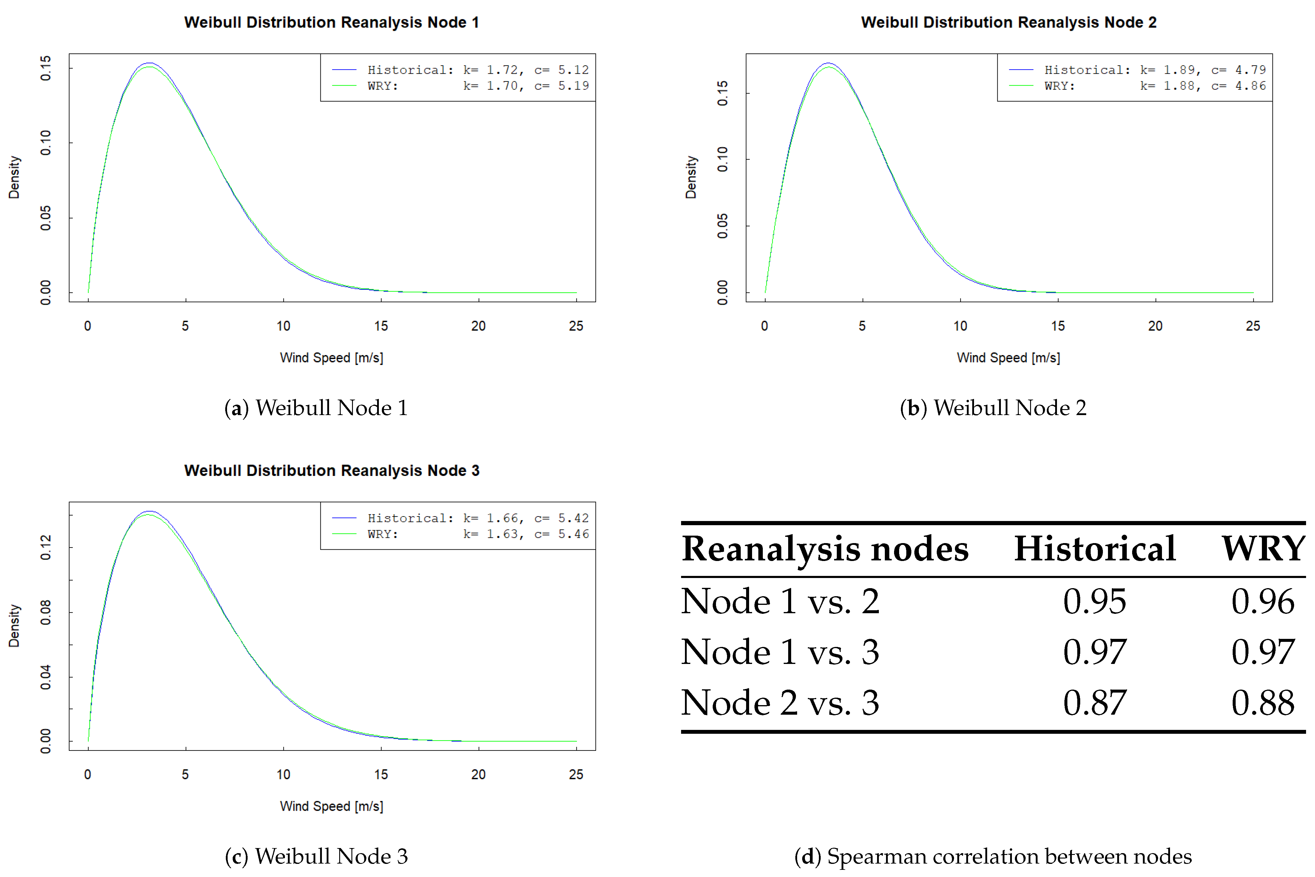
Subsequently, in Figure 3d, the Spearman correlations between the three reanalysis nodes are reported. Furthermore, the Weibull distribution is fitted to historical data from the reanalysis nodes and to the WRY (before site adjustment) in Figure 3a–c.

It is confirmed that the relationship among the variables considered (the wind speeds at the three nodes) is preserved: the Spearman coefficients are practically identical in both cases (Vn1–Vn2 = 0.95 vs. 0.96; Vn1–Vn3 = 0.97 vs. 0.97; Vn2–Vn3 = 0.87 vs. 0.88). Thus, the robust performance of the GMCM in generating synthetic data from the sample is again reinforced.

In the comparison of Weibull distributions, the plots (Figure 3a–c) show that, for each node, the Weibull fit (Equation (1)) to the historical data is very similar to the fit to the simulated data, as are the estimated shape and scale parameters (see Equations (2) and (3)). Therefore, it can be concluded that the GMCM can simulate a distribution similar to that of the original historical reanalysis data.

4.2. WRY Adjusted to the Site

This section analyses the results obtained after adapting the simulated WRY to site conditions. The proposed GMCM method is compared against two baselines—a heuristic month-selection method from the literature and the Windographer commercial workflow. Metrics reported for each approach include Annual Energy Production (AEP), Weibull parameters, and monthly mean wind speeds.

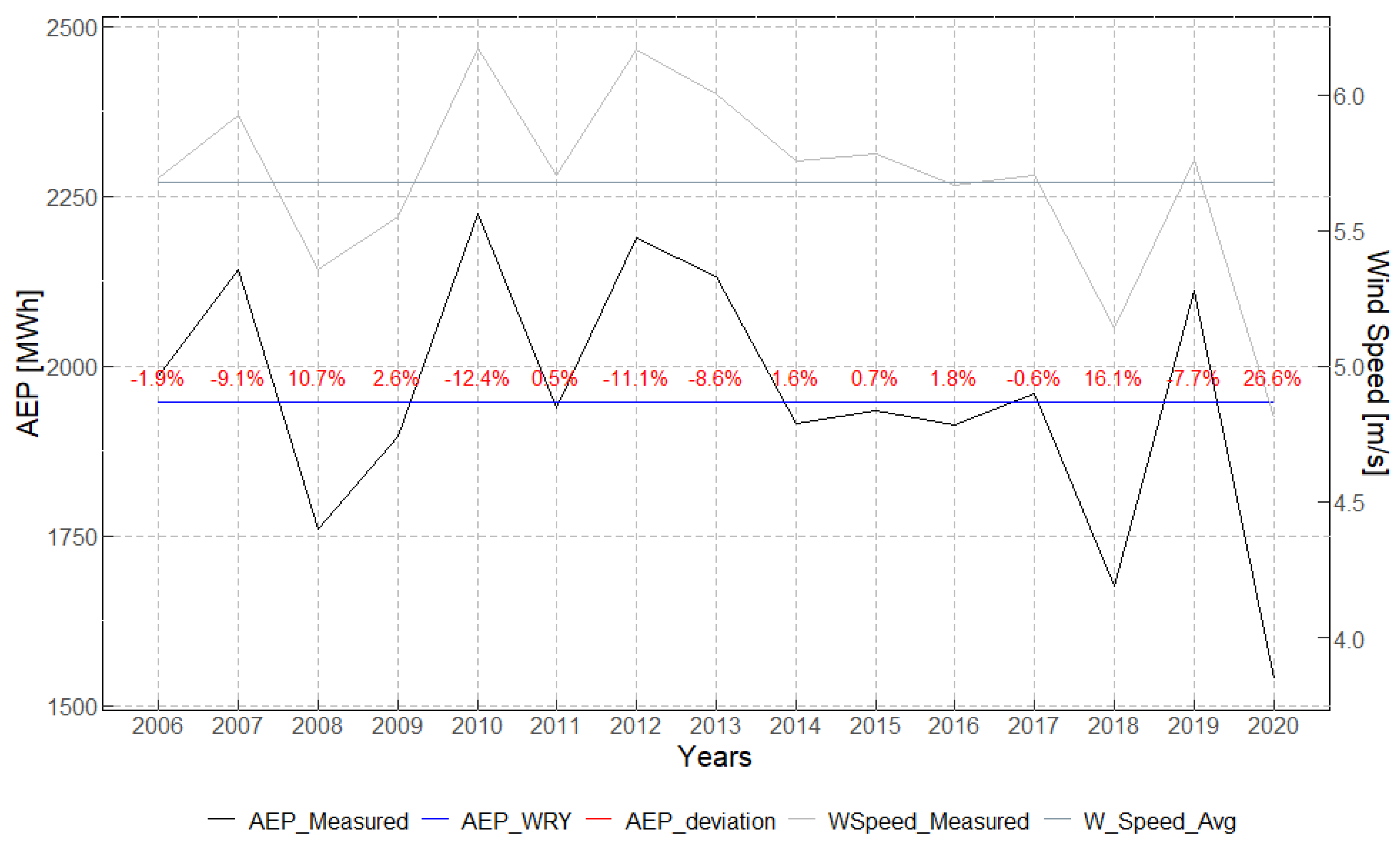
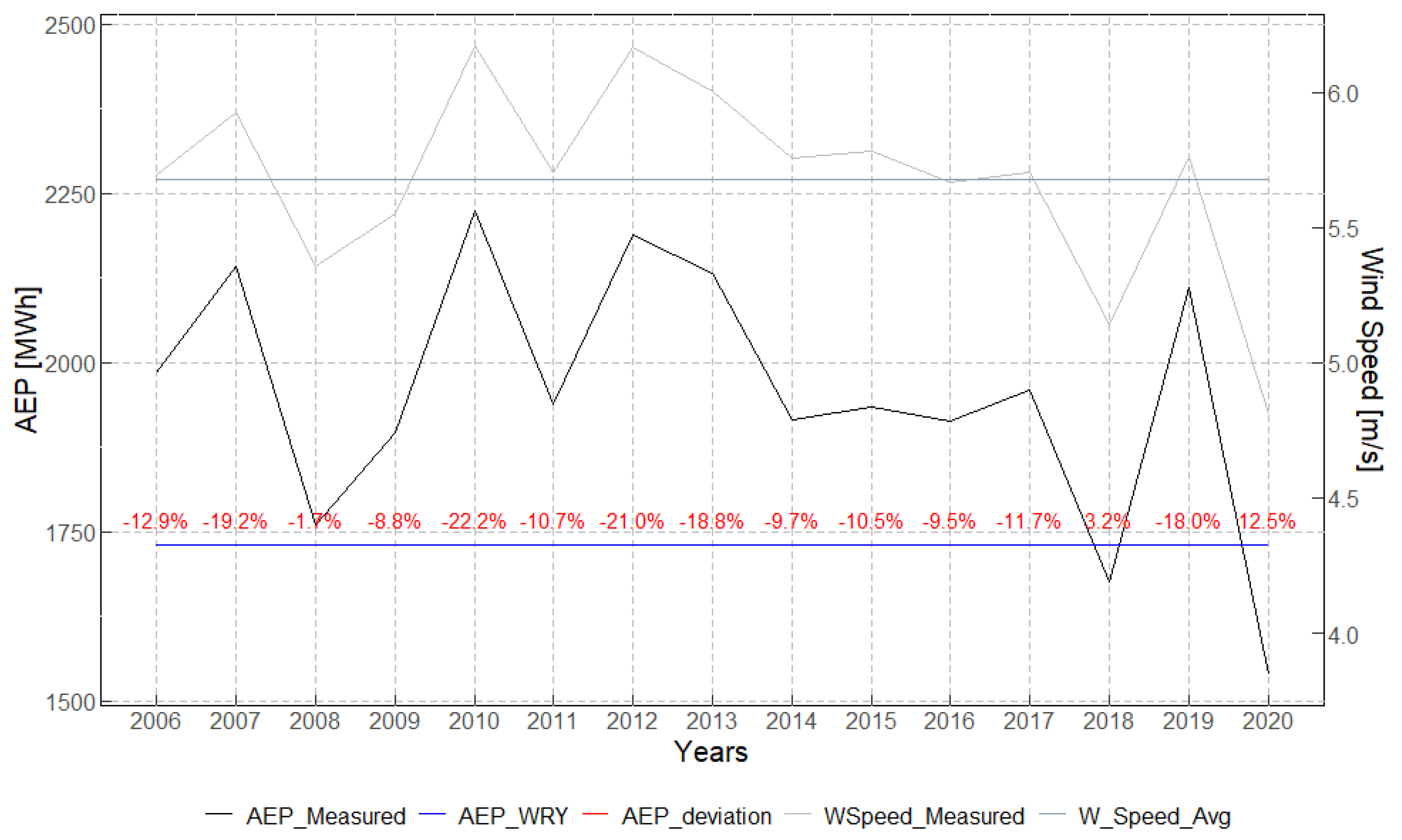
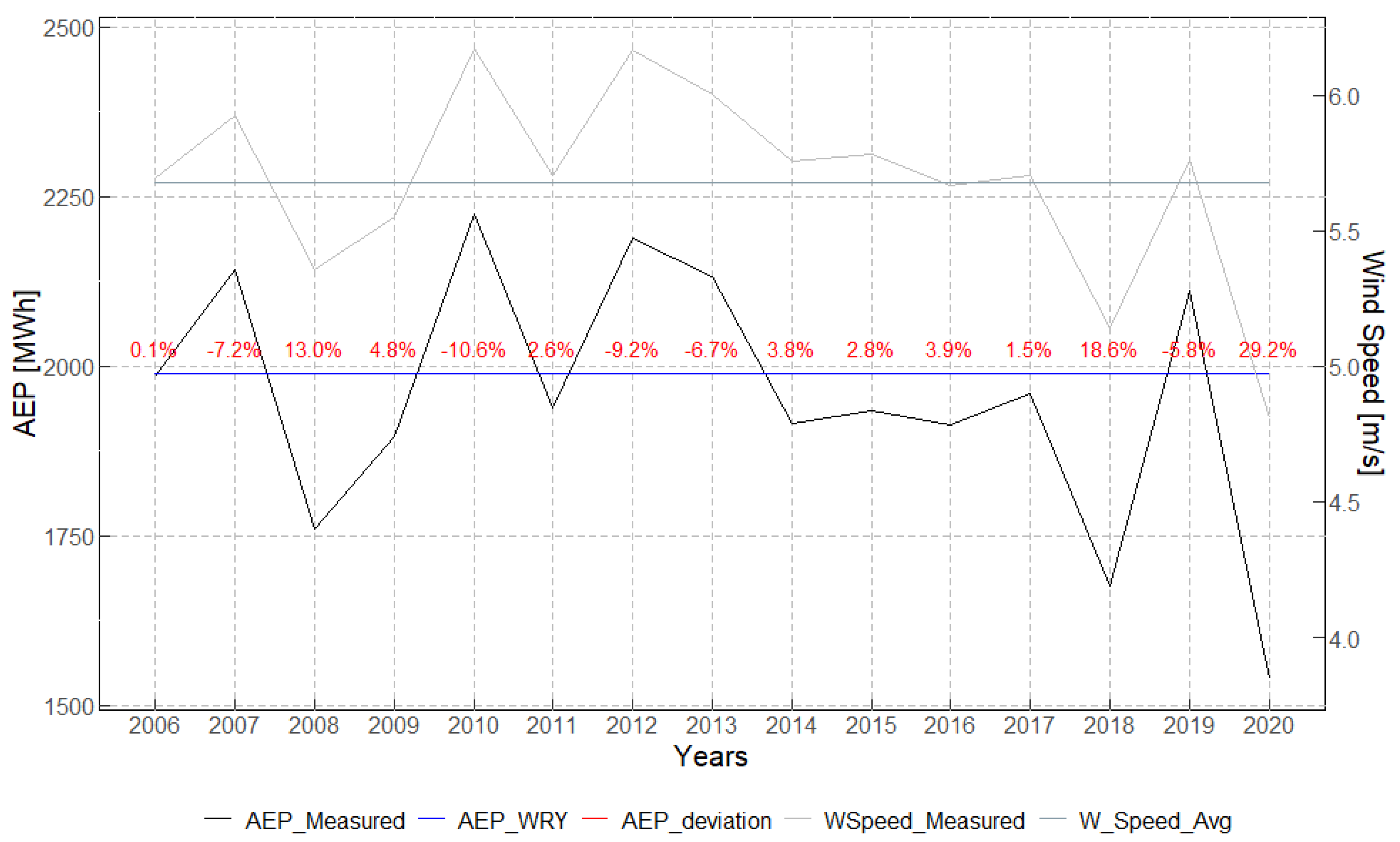
The AEP calculations are shown for the different MCP configurations (see

Table 3. Annual energy production and mean wind speed: GMCM method. Real measurements vs. WRY results.

GMCM Method
MCP Model	Measured AEP [MWh]	WRY-Calculated AEP [MWh]	Diff [%]
GAM	1954	1933	−1.12%
Random Forest (RF)	1954	1974	0.98%
Gradient Boosting (GBR)	1954	1947	−0.36%
Multivariate Linear Regression (MLR)	1954	2142	9.58%
Huber Regression (HR)	1954	2146	9.78%

,

Table 4. Annual energy production and mean wind speed: Heuristic Euclidean-distance method. Real measurements vs. WRY results.

Heuristic Method (Euclidean Distances)
MCP Model	Measured AEP [MWh]	WRY-Calculated AEP [MWh]	Diff [%]
GBR	1954	1731	−11.45%

and

Table 5. Annual energy production and mean wind speed: Windographer method. Real measurements vs. WRY results.

Windographer Method
MCP Model	Measured AEP [MWh]	WRY Calculated AEP [MWh]	Diff [%]
LLS	1954	1988	1.74%
MTS	1954	1901	−2.71%

). In addition, Figure 4, Figure 5 and Figure 6 compare the WRY-derived AEP with the annual AEP computed from the 15-year operational record. In each figure, the black line represents the annual AEP over the 15 available years, the blue line the AEP estimated from the corresponding WRY, and the red markers the percentage deviation of each year’s AEP from the WRY AEP. For context, the annual mean wind speeds (grey) are shown together with their 15-year average (dark grey).

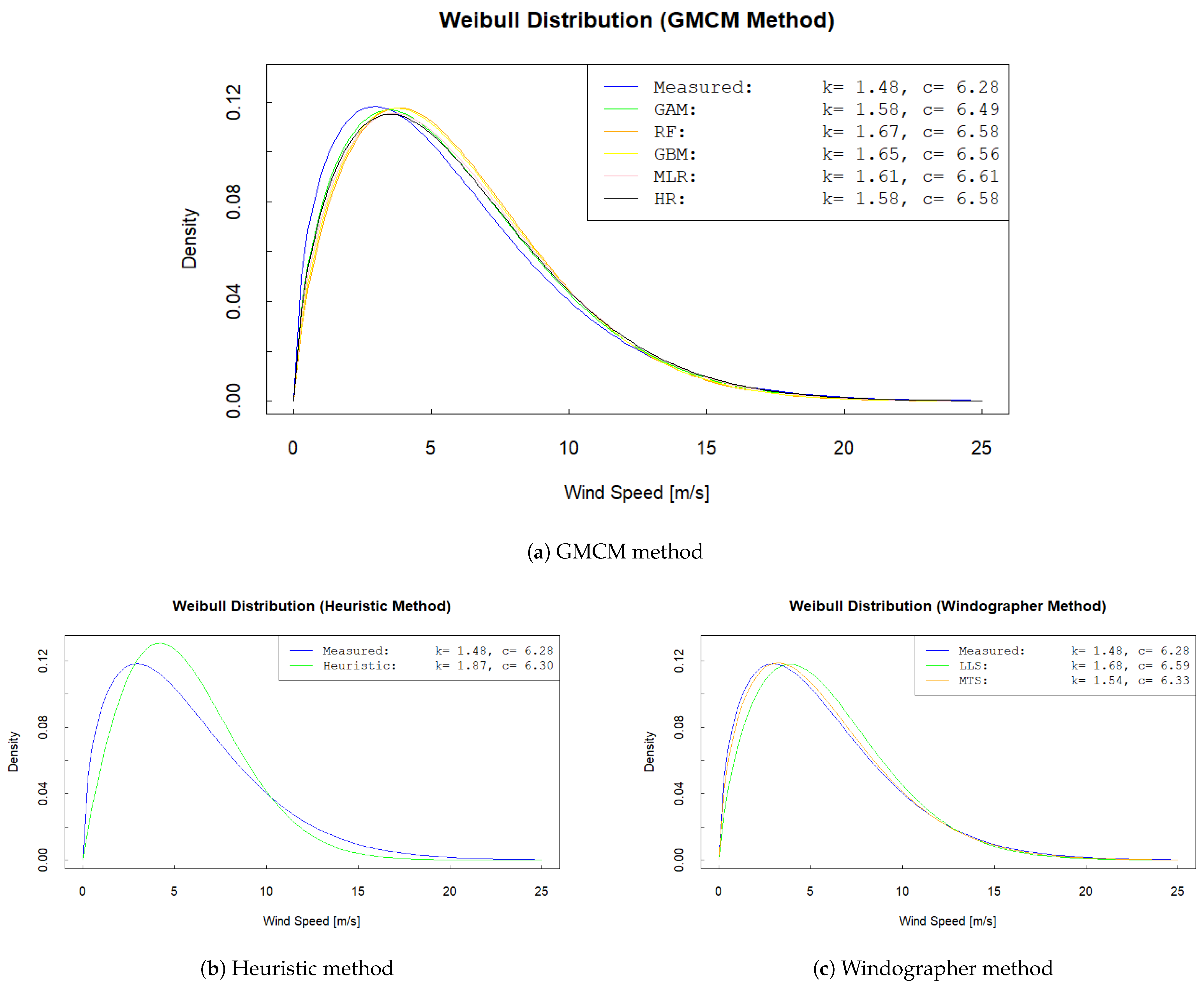
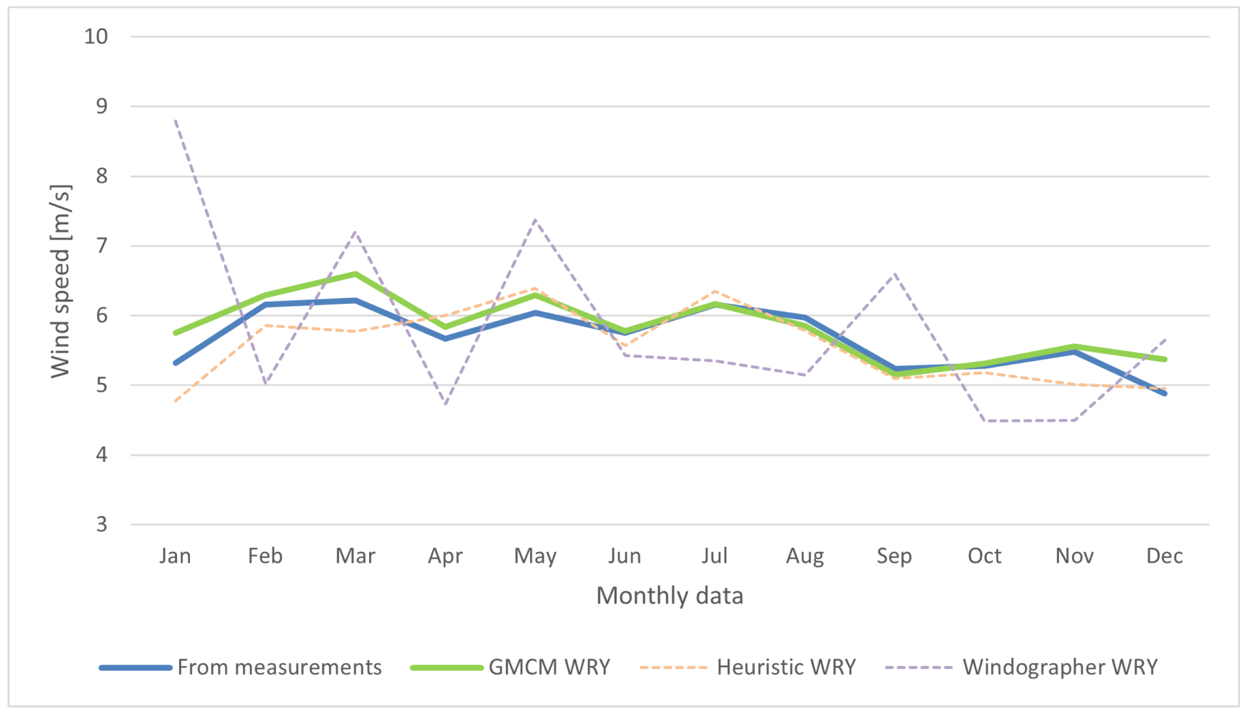
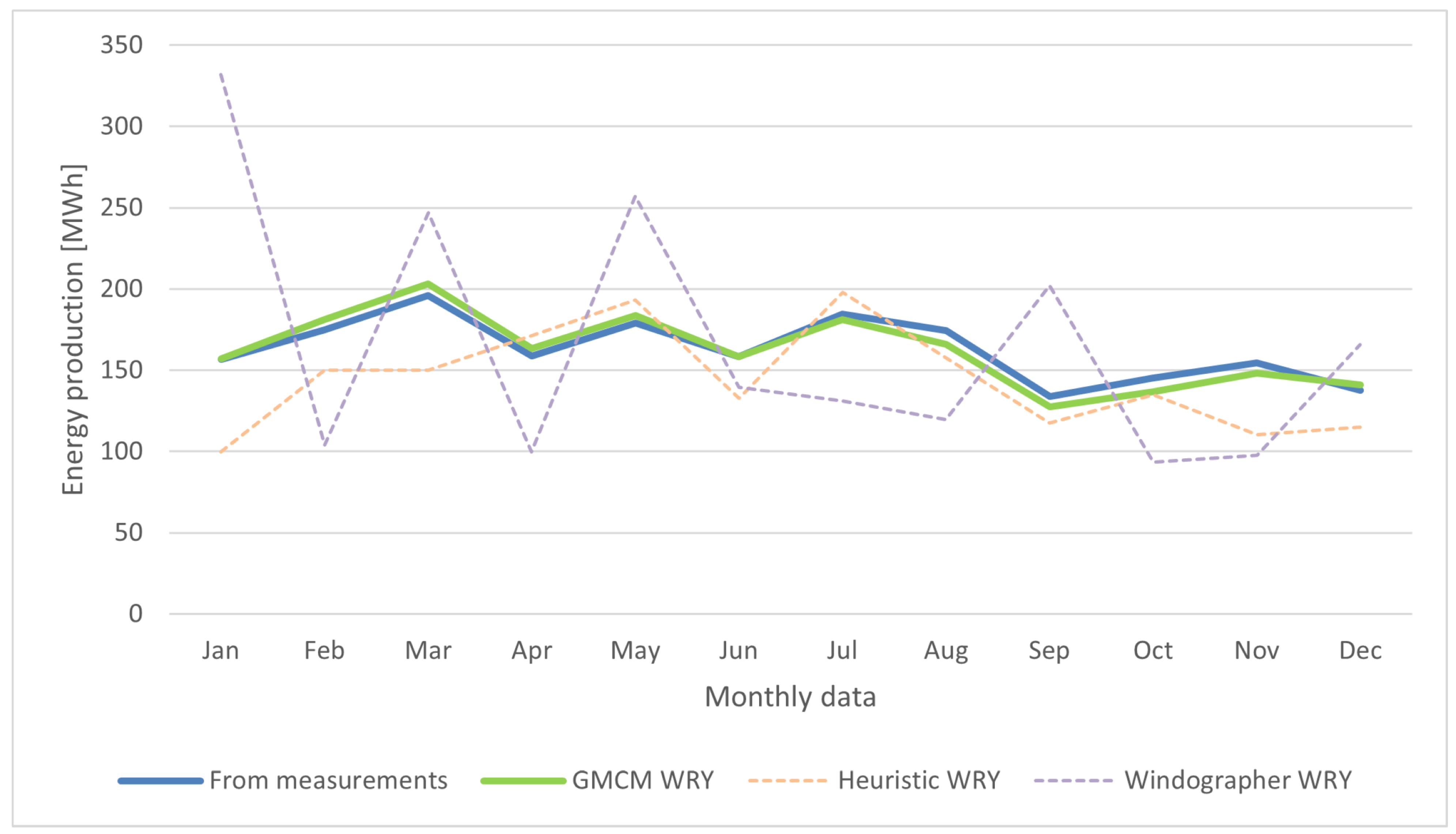
For the Weibull comparison, fitted parameters and the associated Weibull distributions are plotted in Figure 7a–c. Monthly aggregates of mean wind speed and energy (the latter derived from the reference power curve) are provided in

Table 6. Monthly wind speed: Measured compared to WRY and differences by method (GMCM, Heuristic, and Windographer).

	GMCM			Heuristic			Windographer
Month	Wind Speed. Measured [m/s]	Wind Speed. WRY [m/s]	Diff [%]	Wind Speed. Measured [m/s]	Wind Speed. WRY [m/s]	Diff [%]	Wind Speed. Measured [m/s]	Wind Speed. WRY [m/s]	Diff [%]
1	5.32	5.75	−7.54	5.32	4.78	11.27	5.32	8.79	−39.52
2	6.16	6.29	−1.99	6.16	5.86	5.05	6.16	5.02	22.72
3	6.22	6.60	−5.77	6.22	5.77	7.69	6.22	7.20	−13.65
4	5.67	5.84	−3.07	5.67	6.00	−5.62	5.67	4.73	19.66
5	6.04	6.29	−4.08	6.04	6.39	−5.51	6.04	7.37	−18.05
6	5.75	5.78	−0.55	5.75	5.57	3.19	5.75	5.43	5.96
7	6.16	6.17	−0.10	6.16	6.35	−2.97	6.16	5.35	15.22
8	5.97	5.85	2.05	5.97	5.78	3.42	5.97	5.15	16.02
9	5.24	5.15	1.61	5.24	5.10	2.74	5.24	6.59	−20.51
10	5.28	5.31	−0.57	5.28	5.18	2.04	5.28	4.49	17.55
11	5.48	5.56	−1.47	5.48	5.01	9.34	5.48	4.50	21.66
12	4.88	5.37	−9.10	4.88	4.95	−1.28	4.88	5.65	−13.58

and

Table 7. Monthly energy production: Measured compared to WRY and differences by method (GMCM, Heuristic, and Windographer).

	GMCM			Heuristic			Windographer
Month	Energy Production. Measured [MWh]	Energy Production. WRY [MWh]	Diff [%]	Energy Production. Measured [MWh]	Energy Production. WRY [MWh]	Diff [%]	Energy Production. Measured [MWh]	Energy Production. WRY [MWh]	Diff [%]
1	156.70	157.19	−0.31	156.70	99.92	56.82	156.70	331.70	−52.76
2	174.91	181.27	−3.51	174.91	149.90	16.68	174.91	103.82	68.47
3	196.14	202.97	−3.36	196.14	149.98	30.78	196.14	247.08	−20.62
4	158.77	163.39	−2.83	158.77	171.23	−7.28	158.77	99.90	58.93
5	179.09	183.66	−2.49	179.09	193.32	−7.36	179.09	256.96	−30.30
6	158.18	158.41	−0.14	158.18	132.80	19.11	158.18	139.45	13.43
7	184.72	181.17	1.96	184.72	198.08	−6.75	184.72	130.88	41.13
8	174.48	165.79	5.24	174.48	157.69	10.65	174.48	119.53	45.98
9	133.97	127.66	4.94	133.97	117.42	14.09	133.97	202.10	−33.71
10	145.38	136.77	6.30	145.38	134.66	7.96	145.38	93.64	55.25
11	154.42	147.99	4.34	154.42	110.52	39.72	154.42	97.71	58.04
12	137.70	141.11	−2.42	137.70	115.05	19.68	137.70	165.72	−16.91

and visualised in Figure 8 and Figure 9.

For the AEP comparison, the average annual energy from the 15-year measured dataset is taken as the benchmark and compared with the AEP obtained from each WRY. Because different regression models are used to adapt wind speed to the site, the resulting AEP varies by method and by model.

For the proposed GMCM-based method, the AEP differences range from $-0.36\%$ to $+9.78\%$ across the regression models tested. The best results are obtained with Random Forest (RF) and Gradient Boosting Regressor (GBR), yielding AEP errors of $+0.98\%$ and $-0.36\%$, respectively, whereas Multivariate Linear Regression (MLR) and Huber Regression (HR) show the largest positive biases. For the year-by-year comparison, we focus on the best case (GBR). As shown in Figure 4, deviations with respect to the WRY AEP range from $0.5\%$ to $26\%$; overall, this method most closely aligns with the 15-year average behaviour. The largest discrepancies correspond to years with unusually low or high wind resources (notably 2020 in this dataset). Despite year-to-year variability, the WRY estimate remains consistent with the long-term mean.

Regarding the heuristic baseline where a single Gradient-Boosting-based MCP model is applied, the AEP difference is substantial ($-11.45\%$). This outcome is consistent with expectations: although a month is selected from the historical record to resemble long-term behaviour, its characteristics are not identical to the long-term climatology, so deviations are anticipated. Figure 5 shows that the WRY AEP obtained with this method differs from the annual AEP values derived from the 15-year record by between 3% and 22%, depending on the year.

For the Windographer baseline, the AEP differences are $+1.74\%$ when using the Linear Least Squares (LLS) option and $-2.71\%$ with the Matrix Time Series (MTS) option provided in Windographer’s MCP module. For the year-by-year comparison, we focus on the best case (LLS). As shown in Figure 6, the deviations with respect to the WRY AEP range from $0.1\%$ to $29\%$; in general, the WRY estimate follows the multi-year average behaviour. The largest discrepancies occur in years with unusually low or high wind resources relative to the rest of the period.

In terms of AEP estimation, the best overall performance is achieved by the GMCM method combined with the GBR regression model for site adaptation.

In the comparison of Weibull distributions fitted to the real (measured) data and to the simulated WRY, similar conclusions are obtained. For the Heuristic method, the Weibull fit for the WRY differs slightly from the fit to the measured data (Figure 7b). This is expected because the selected month from the historical record has characteristics that are close to, but not identical with, the long-term climatology.

By contrast, the fits for the GMCM and Windographer methods are much closer to the measured distribution (Figure 7a,c). Both methods deliver an accurate representation of the site’s wind-speed distribution, with the MTS option in Windographer performing slightly better than the GBR-based case in GMCM. These outcomes emphasise the importance of the MCP method and, additionally, highlight the impact of reanalysis-data quality on the final result.

Once the best-performing case within each method has been identified, the analysis centers on the proposed GMCM method (with GBR-based MCP) and, for context, two baselines: the heuristic month-selection approach (Euclidean distance) and the Windographer workflow (LLS-based MCP). A monthly analysis of wind speed and energy is presented. Comparative tables report monthly mean wind speed and monthly energy production, and in all cases, the WRY-derived monthly series are contrasted with the 15-year measured aggregates.

Table 6 and Table 7 summarize the monthly averages of wind speed and the corresponding monthly energy (computed with the site’s reference power curve) for the best-case configuration of the proposed GMCM method and for the two baselines—the heuristic approach and Windographer (best-case MCP option). For each month of a typical year, the tables report the deviation of the WRY-derived values from the 15-year measured aggregates.

The final outcome of the process is an hourly wind-speed time series that exhibits the hallmarks of a realistic wind pattern—persistence together with seasonal and diurnal variability. Moreover, the series can be regarded as representative of the site’s long-term behaviour.

In the proposed GMCM workflow, the simulated values are temporally reordered using the Hungarian algorithm to enforce persistence and realistic sequencing (see Section 3.3). The resulting 8760 h WRY is therefore suitable for direct use in standard industry tools for energy assessment. For the proposed GMCM method, wind-speed deviations are ∼$0.1$–$9\%$, and production deviations are ∼0.1–$6.3\%$ (absolute percentage). For the heuristic baseline, wind-speed deviations are approximately $1.3$–$11.2\%$, while production deviations are ∼7–$56\%$ (absolute percentage). For the Windographer baseline, wind-speed deviations are ∼6–$40\%$, with production deviations of ∼13–$69\%$ (absolute percentage). These deviations should also be interpreted in the context of typical uncertainty levels associated with long-term resource assessment. Recent studies report that wind-resource uncertainty alone can introduce AEP variations of ∼0.4–$3.7\%$ in operational offshore projects [4], indicating that the deviations obtained with the proposed WRY fall well within the expected range for real-world applications. These results confirm that, for both wind speed and energy, the proposed method attains the lowest monthly deviations, as also illustrated in Figure 8 and Figure 9, where the WRY monthly wind speeds and the WRY monthly productions are compared against the 15-year measured aggregates.

5. Conclusions

This work demonstrates a method to estimate a Wind Reference Year (WRY) from fifteen years of reanalysis data combined with a one-year on-site measurement campaign. Results are compared against two practical alternatives: a heuristic month-selection approach based on practitioner expertise and the commercial Windographer workflow.

From the obtained results, we infer that the proposed method—based on Gaussian Mixture Copula Models (GMCMs)—captures long-term wind behaviour and can generate synthetic series suitable for WRY estimation. Moreover, applying the Hungarian algorithm to temporally reassign the simulated values ensures that the final series respects wind persistence and exhibits a realistic seasonal and diurnal pattern.

Site adaptation remains a challenging step. Several regression models were evaluated (GAM, RF, GBR, MLR, and HR). In this case study, the Gradient Boosting Regressor (GBR) provided the best performance, with an AEP deviation of approximately 0.3% relative to the multi-year measurements. The quality of the long-term reference and the strength of correlation between measured and reanalysis data are critical to achieving robust outcomes. Although the energy results are satisfactory, there is still room for improvement in the transposition from reanalysis to site conditions.

As with any typical-year construction, the proposed WRY is not intended to reproduce event-scale dynamics, such as gusts or abrupt regime transitions, since these behaviours are inherently smoothed when condensing multi-year data into a representative year. The method may also face limitations at sites where reanalysis nodes exhibit weak correlation with local measurements or in environments affected by strong non-stationarity, where long-term representativeness becomes more difficult to achieve. These aspects define natural boundaries of applicability and point to opportunities for methodological refinement.

Future work will consider higher-quality long-term references from meteorological reanalyses (e.g., the global meteorological reanalysis model Vortex) and additional site-adaptation strategies. In parallel, to support hybrid plant design, the WRY dataset should be extended to incorporate other renewable resources (e.g., solar) while preserving their joint dependence structure within a common, multi-source reference year. This will enable consistent, multi-vector resource assessments that remain faithful to the temporal co-variability required by modern hybrid systems.

References

1. REN21. Renewables 2023 Global Status Report. Technical Report, Renewable Energy Policy Network for the 21st Century (REN21). 2023. Available online: https://www.ren21.net/reports/global-status-report/ (accessed on 8 September 2025).
2. Habbou, H.; Leon, J.P.M.; Das, K. Profitability of hybrid power plants in European markets. J. Phys. Conf. Ser. 2023, 2507, 012009. [Google Scholar] [CrossRef]
3. Lee, J.; Fields, J. An overview of wind-energy-production prediction bias, losses, and uncertainties. Wind. Energy Sci. 2021, 6, 311–365. [Google Scholar] [CrossRef]
4. Klemmer, K.S.; Condon, E.P.; Howland, M.F. Evaluation of wind resource uncertainty on energy production estimates for offshore wind farms. J. Renew. Sustain. Energy 2024, 16, 013302. [Google Scholar] [CrossRef]
5. Pernigotto, G.; Prada, A.; Cóstola, D.; Gasparella, A.; Hensen, J.L. Multi-year and reference year weather data for building energy labelling in north Italy climates. Energy Build. 2014, 72, 62–72. [Google Scholar] [CrossRef]
6. Pernigotto, G.; Prada, A.; Gasparella, A.; Hensen, J.L. Analysis and improvement of the representativeness of EN ISO 15927-4 reference years for building energy simulation. J. Build. Perform. Simul. 2014, 7, 391–410. [Google Scholar] [CrossRef]
7. Cebecauer, T.; Suri, M. Typical Meteorological Year Data: SolarGIS Approach. Energy Procedia 2015, 69, 1958–1969. [Google Scholar] [CrossRef]
8. Janjai, S.; Deeyai, P. Comparison of methods for generating typical meteorological year using meteorological data from a tropical environment. Appl. Energy 2009, 86, 528–537. [Google Scholar] [CrossRef]
9. Wu, Y.; An, J.; Gui, C.; Xiao, C.; Yan, D. A global typical meteorological year (TMY) database on ERA5 dataset. Build. Simul. 2023, 16, 1013–1026. [Google Scholar] [CrossRef]
10. Tang, Y.; Sun, T.; Luo, Z.; Omidvar, H.; Theeuwes, N.; Xie, X.; Xiong, J.; Yao, R.; Grimmond, S. Urban meteorological forcing data for building energy simulations. Build. Environ. 2021, 204, 108088. [Google Scholar] [CrossRef]
11. Hall, I.J.; Prairie, R.R.; Anderson, H.E.; Boes, E.C. Generation of Typical Meteorological Years for 26 SOLMET Stations; Technical Report SAND-78-1096C; CONF-780639-1; Sandia National Laboratories: Albuquerque, NM, USA, 1978.
12. Marion, W.; Urban, K. User’s Manual for TMY2s (Typical Meteorological Years)—Derived from the 1961–1990 National Solar Radiation Data Base; Technical Report NREL/TP-463-7668; National Renewable Energy Laboratory (NREL): Golden, CO, USA, 1995. [CrossRef]
13. Wilcox, S.; Marion, W. Users Manual for TMY3 Data Sets; Technical Report NREL/TP-581-43156; National Renewable Energy Laboratory: Golden, CO, USA, 2008. [CrossRef]
14. Abreu, E.F.; Canhoto, P.; Prior, V.; Melicio, R. Solar resource assessment through long-term statistical analysis and typical data generation with different time resolutions using GHI measurements. Renew. Energy 2018, 127, 398–411. [Google Scholar] [CrossRef]
15. Pusat, S.; Karagöz, Y. A new reference wind year approach to estimate long term wind characteristics. Adv. Mech. Eng. 2021, 13, 16878140211021268. [Google Scholar] [CrossRef]
16. Hersbach, H.; Bell, B.; Berrisford, P.; Biavati, G.; Horányi, A.; Muñoz Sabater, J.; Nicolas, J.; Peubey, C.; Radu, R.; Rozum, I.; et al. ERA5 Hourly Data on Single Levels from 1959 to Present. Copernicus Climate Change Service (C3S) Climate Data Store (CDS). 2018. Available online: https://cds.climate.copernicus.eu/datasets/reanalysis-era5-single-levels?tab=overview (accessed on 9 December 2025). [CrossRef]
17. Gualtieri, G. Reliability of ERA5 Reanalysis Data for Wind Resource Assessment: A Comparison against Tall Towers. Energies 2021, 14, 4169. [Google Scholar] [CrossRef]
18. Cannon, A.J.; Sobie, S.R.; Murdock, T.Q. Bias correction of GCM precipitation by quantile mapping: How well do methods preserve changes in quantiles and extremes? J. Clim. 2015, 28, 6938–6959. [Google Scholar] [CrossRef]
19. Cannon, A.J. Multivariate bias correction of climate model output: Matching marginal distributions and intervariable dependence structure. J. Clim. 2016, 29, 7045–7064. [Google Scholar] [CrossRef]
20. Gualtieri, G. Analysing the uncertainties of reanalysis data used for wind resource assessment: A critical review. Renew. Sustain. Energy Rev. 2022, 167, 112741. [Google Scholar] [CrossRef]
21. Cosculluela Soteras, L.; Llombart Estopiñán, A.; Pueyo Rufas, C. Estudio del Impacto de Diferentes Técnicas de Medición-Correlación-Predicción Sobre la Producción Eléctrica en Parques Eólicos. [Recurso Electrónico]; Engineering Final Project CD 1078; Universidad de Zaragoza, Centro Politécnico Superior: Zaragoza, Spain, 2008. [Google Scholar]
22. Beltran, J.; Cosculluela, L.; Pueyo, C.; Melero, J.J. Comparison of measure-correlate-predict methods in wind resource assessments. In Proceedings of the European Wind Energy Conference and Exhibition (EWEC 2010), Warsaw, Poland, 20–23 April 2010; pp. 3280–3286. [Google Scholar]
23. Carta, J.A.; Velázquez, S.; Cabrera, P. A review of measure-correlate-predict (MCP) methods used to estimate long-term wind characteristics at a target site. Renew. Sustain. Energy Rev. 2013, 27, 362–400. [Google Scholar] [CrossRef]
24. Measuring Network of Wind Energy Institutes (MEASNET). Evaluation of Site-Specific Wind Conditions. 2016. Available online: https://www.measnet.com/wp-content/uploads/2016/05/Measnet_SiteAssessment_V2.0.pdf (accessed on 9 December 2025).
25. Carta, J.A.; Moreno, D.; Cabrera, P. A Measure–Correlate–Predict Approach for Transferring Wind Speeds from MERRA2 Reanalysis to Wind Turbine Hub Heights. J. Mar. Sci. Eng. 2025, 13, 1213. [Google Scholar] [CrossRef]
26. Pérez-Pérez, E.J.; López-Estrada, F.R.; Puig, V.; Valencia-Palomo, G.; Santos-Ruiz, I. Fault diagnosis in wind turbines based on ANFIS and Takagi–Sugeno interval observers. Expert Syst. Appl. 2022, 206, 117698. [Google Scholar] [CrossRef]
27. Pérez-Pérez, E.J.; Puig, V.; López-Estrada, F.R.; Valencia-Palomo, G.; Santos-Ruiz, I.; Osorio-Gordillo, G. Robust fault diagnosis of wind turbines based on MANFIS and zonotopic observers. Expert Syst. Appl. 2024, 235, 121095. [Google Scholar] [CrossRef]
28. Joint Research Centre (JRC), the European Commission’s Science and Knowledge Service. PVGIS Photovoltaic Geographical Information System. 2020. Available online: https://joint-research-centre.ec.europa.eu/pvgis-photovoltaic-geographical-information-system_en (accessed on 9 December 2025).
29. Huld, T.; Paietta, E.; Zangheri, P.; Pinedo Pascua, I. Assembling Typical Meteorological Year Data Sets for Building Energy Performance Using Reanalysis and Satellite-Based Data. Atmosphere 2018, 9, 53. [Google Scholar] [CrossRef]
30. UNE-EN ISO 15927-4; Hygrothermal Performance of Buildings—Calculation and Presentation of Climatic Data—Part 4: Hourly Data for Assessing the Annual Energy Use for Heating and Cooling. AENOR: Madrid, Spain, 2011.
31. UL Solutions. Windographer. Wind Data Analytics and Visualization Solution. 2022. Available online: https://www.ul.com/services/windographer-wind-data-analytics-and-visualization-solution (accessed on 14 September 2022).
32. Bilgrau, A.E.; Eriksen, P.S.; Rasmussen, J.G.; Johnsen, H.E.; Dybkaer, K.; Boegsted, M. GMCM: Unsupervised Clustering and Meta-Analysis Using Gaussian Mixture Copula Models. J. Stat. Softw. 2016, 70, 1–23. [Google Scholar] [CrossRef]
33. Meyer, D.; Nagler, T.; Hogan, R.J. Copula-based synthetic data augmentation for machine-learning emulators. Geosci. Model Dev. 2021, 14, 5205–5215. [Google Scholar] [CrossRef]
34. Yoo, J.; Son, Y.; Yoon, M.; Choi, S. A Wind Power Scenario Generation Method Based on Copula Functions and Forecast Errors. Sustainability 2023, 15, 16536. [Google Scholar] [CrossRef]
35. Srinivas, V.V.; Srinivasan, K. Hybrid Moving Block Bootstrap for Stochastic Simulation of Multi-Site Multi-Season Streamflows. J. Hydrol. 2005, 302, 307–330. [Google Scholar] [CrossRef]
36. Marcon, G.; Marletta, A.; Moradi, S.; Zizzo, G.; Favuzza, S.; Sottile, G. Time Series Bootstrap for Renewable Energy Analysis in Power Grid Optimization. In Statistics for Innovation III; di Bella, E., Gioia, V., Lagazio, C., Zaccarin, S., Eds.; Italian Statistical Society Series on Advances in Statistics; Springer: Cham, Switzerland, 2025; pp. 463–468. [Google Scholar] [CrossRef]
37. Turowski, M.; Heidrich, B.; Weingärtner, L.; Springer, L.; Phipps, K.; Schäfer, B.; Mikut, R.; Hagenmeyer, V. Generating Synthetic Energy Time Series: A Review. Renew. Sustain. Energy Rev. 2024, 206, 114842. [Google Scholar] [CrossRef]
38. Wu, L.; Zhang, Y.; Adams, T.; Lee, H.; Liu, Y.; Schaake, J. Comparative Evaluation of Three Schaake Shuffle Schemes in Postprocessing GEFS Precipitation Ensemble Forecasts. J. Hydrometeorol. 2018, 19, 575–598. [Google Scholar] [CrossRef]
39. Shrestha, D.L.; Robertson, D.E.; Bennett, J.C.; Wang, Q.J. Using the Schaake Shuffle When Calibrating Ensemble Means Can Be Problematic. J. Hydrol. 2020, 587, 124991. [Google Scholar] [CrossRef]
40. Alessandrini, S.; McCandless, T. The Schaake Shuffle Technique to Combine Solar and Wind Power Probabilistic Forecasting. Energies 2020, 13, 2503. [Google Scholar] [CrossRef]
41. Naimo, A. A Novel Approach to Generate Synthetic Wind Data. Procedia-Soc. Behav. Sci. 2014, 108, 187–196. [Google Scholar] [CrossRef]
42. Jung, C.; Schindler, D. The role of the power law exponent in wind energy assessment: A global analysis. Int. J. Energy Res. 2021, 45, 8484–8496. [Google Scholar] [CrossRef]
43. Meucci, A. A Short, Comprehensive, Practical Guide to Copulas. GARP Risk Professional. 2011, pp. 22–27. Available online: https://papers.ssrn.com/sol3/papers.cfm?abstract_id=1847864 (accessed on 9 December 2025).
44. Shahirinia, A.; Farahmandfar, Z.; Tavakoli Bina, M.; Henderson, S.B.; Ashtary, M. Spatial modeling sensitivity analysis: Copula selection for wind speed dependence. AIP Adv. 2024, 14, 045047. [Google Scholar] [CrossRef]
45. Kasa, R.; Rajan, V.K. Improved Inference of Gaussian Mixture Copula Model for Clustering and Reproducibility Analysis using Automatic Differentiation. Econom. Stat. 2022, 22, 67–97. [Google Scholar] [CrossRef]
46. Salehi Borujeni, M.; Dideban, A.; Akbari Foroud, A. Reconstructing long-term wind speed data based on measure correlate predict method for micro-grid planning. J. Ambient. Intell. Humaniz. Comput. 2021, 12, 10183–10195. [Google Scholar] [CrossRef]
47. Chen, D.; Zhou, Z.; Yang, X. A measure–correlate–predict model based on neural networks and frozen flow hypothesis for wind resource assessment. Phys. Fluids 2022, 34, 045107. [Google Scholar] [CrossRef]
48. Bergstra, J.; Bengio, Y. Random search for hyper-parameter optimization. J. Mach. Learn. Res. 2012, 13, 281–305. [Google Scholar]
49. Chambers, J.; Hastie, T.; Pregibon, D. Statistical Models in S. In Compstat; Momirović, K., Mildner, V., Eds.; Physica-Verlag HD: Heidelberg, Germany, 1990; pp. 317–321. [Google Scholar] [CrossRef]
50. Hastie, T.; Tibshirani, R. Generalized Additive Models; Chapman and Hall: London, UK, 1990; p. 352. [Google Scholar] [CrossRef]
51. Ridgeway, G. The State of Boosting. In Computing Science and Statistics; Interface Foundation of North America: Fairfax Station, VA, USA, 1999; Volume 31, pp. 172–181. [Google Scholar]
52. Breiman, L. Random Forests. Mach. Learn. 2001, 45, 5–32. [Google Scholar] [CrossRef]
53. Huber, P.J. Robust Statistics. In International Encyclopedia of Statistical Science; Lovric, M., Ed.; Springer: Berlin/Heidelberg, Germany, 2011; pp. 1248–1251. [Google Scholar] [CrossRef]
54. Justus, C.G.; Hargraves, W.R.; Mikhail, A.; Graber, D. Methods for Estimating Wind Speed Frequency Distributions. J. Appl. Meteorol. 1978, 17, 350–353. [Google Scholar] [CrossRef]
55. Dodge, Y. (Ed.) Spearman Rank Correlation Coefficient. In The Concise Encyclopedia of Statistics; Springer: New York, NY, USA, 2008; pp. 502–505. [Google Scholar] [CrossRef]
56. IEC 61400-12-1:2017; Wind Energy Generation Systems—Part 12-1: Power Performance Measurements of Electricity Producing Wind Turbines. International Electrotechnical Commission (IEC): Geneva, Switzerland, 2017.
Figure 2. Data reordering from GMCM simulation adapted to the site (sample of one month).
Applsci 15 13147 g002
Figure 3. Weibull distributions from historical reanalysis data compared with WRY data.
Applsci 15 13147 g003
Figure 4. GMCM method: Actual yearly AEP (black) vs. WRY-calculated AEP (blue). Red markers show the percentage deviation. Annual mean wind speeds (grey) and their 15-year average (dark grey) are shown for context.
Applsci 15 13147 g004
Figure 5. Heuristic method: Actual yearly AEP (black) vs. WRY-calculated AEP (blue). Red markers show the percentage deviation. Annual mean wind speeds (grey) and their 15-year average (dark grey) are shown for context.
Applsci 15 13147 g005
Figure 6. Windographer method: Actual yearly AEP (black) vs. WRY-calculated AEP (blue). Red markers show the percentage deviation. Annual mean wind speeds (grey) and their 15-year average (dark grey) are shown for context.
Applsci 15 13147 g006
Figure 7. Weibull distributions adapted to the site for the three methodologies.
Applsci 15 13147 g007
Figure 8. Monthly wind speed: Mast measurements compared to the estimated from the WRY for three methods (GMCM, Heuristic, and Windographer).
Applsci 15 13147 g008
Figure 9. Monthly energy production: Estimated from mast measurements compared to the estimated from the WRY for three methods (GMCM, Heuristic, and Windographer).
Applsci 15 13147 g009