Author Contributions
Conceptualization, S.A. and D.C.; methodology, S.A.; software, S.A. and Y.K.; validation, S.A. and D.C. (Dongyoung Choi); formal analysis, D.C. (Dongyoung Choi); investigation, D.C. (Dongyoung Choi); resources, S.A.; data curation, S.C. and S.A.; writing—original draft preparation, S.A.; writing—review and editing, D.C. (Dongil Choi); visualization, S.C. and Y.K.; supervision, D.C. (Dongil Choi); project administration, D.C. (Dongil Choi); funding acquisition, D.C. (Dongil Choi). All authors have read and agreed to the published version of the manuscript.
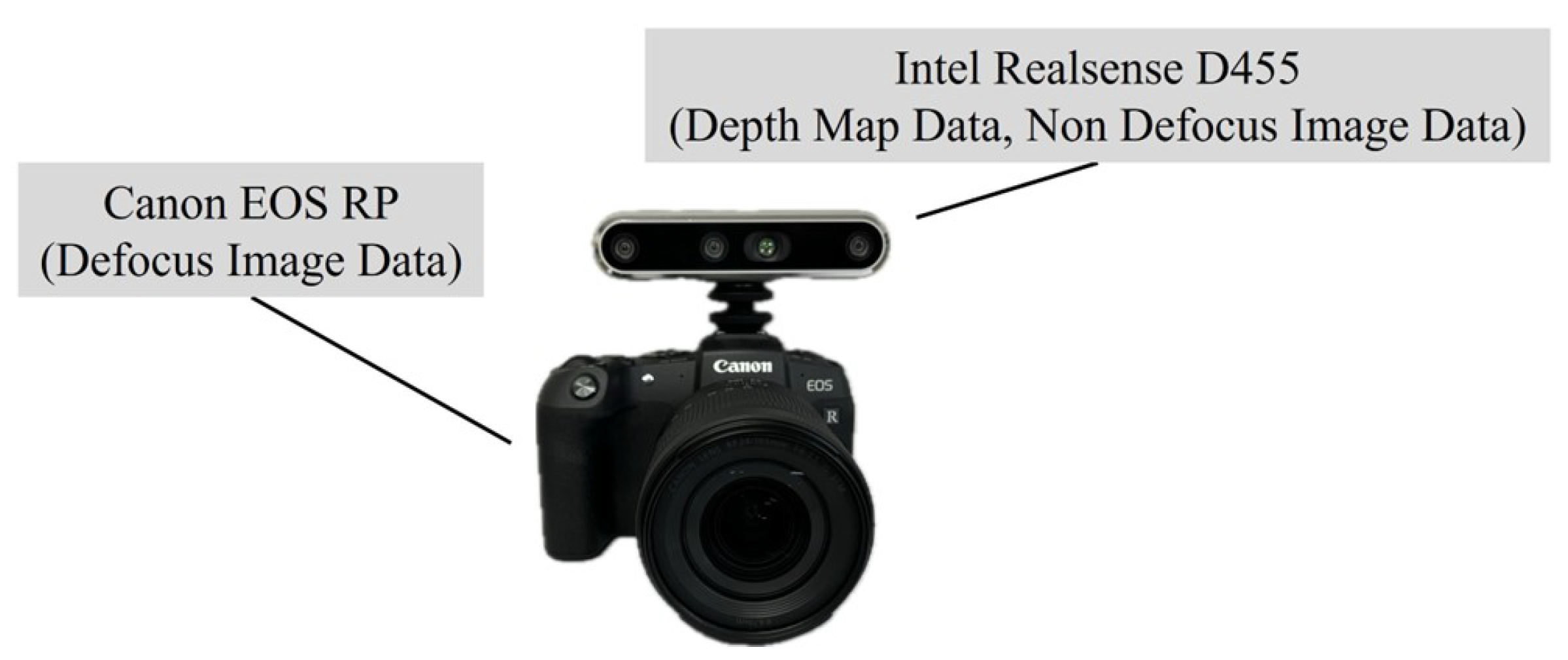
Figure 1.
Data collection hardware.
Figure 1.
Data collection hardware.
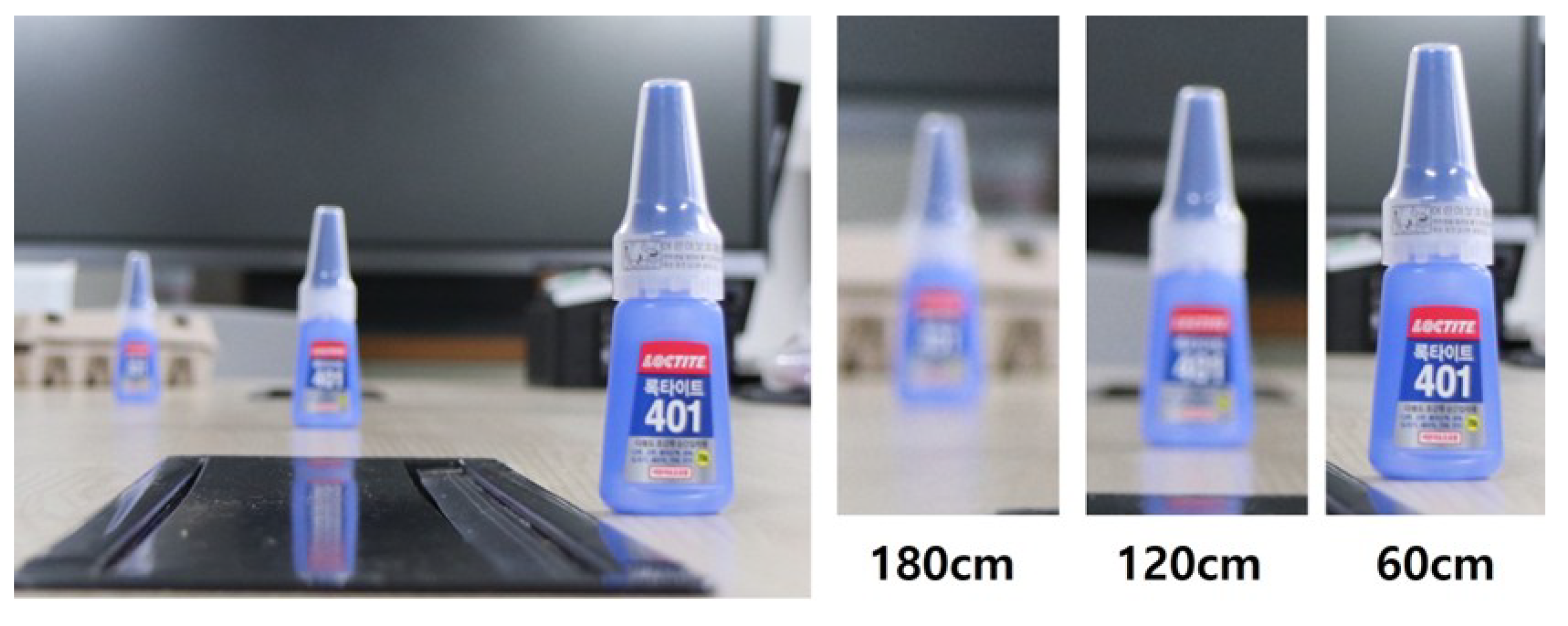
Figure 2.
Compare the degree of blur based on distance (from left to right, 180 cm, 120 cm, 60 cm).
Figure 2.
Compare the degree of blur based on distance (from left to right, 180 cm, 120 cm, 60 cm).
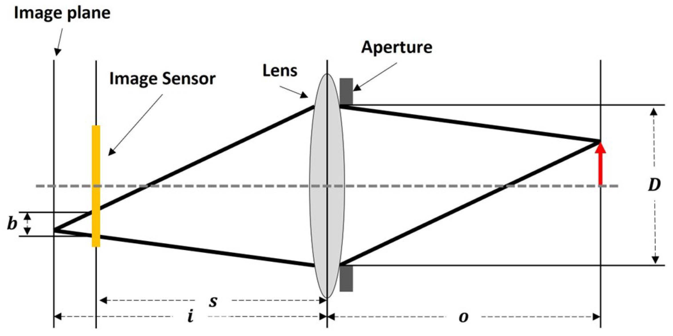
Figure 3.
Cross-section of a thin lens.
Figure 3.
Cross-section of a thin lens.
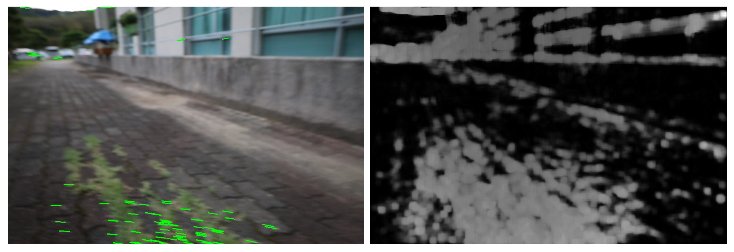
Figure 4.
(Left) Sparse Optical Flow, (Right) Dense Optical Flow.
Figure 4.
(Left) Sparse Optical Flow, (Right) Dense Optical Flow.
Figure 5.
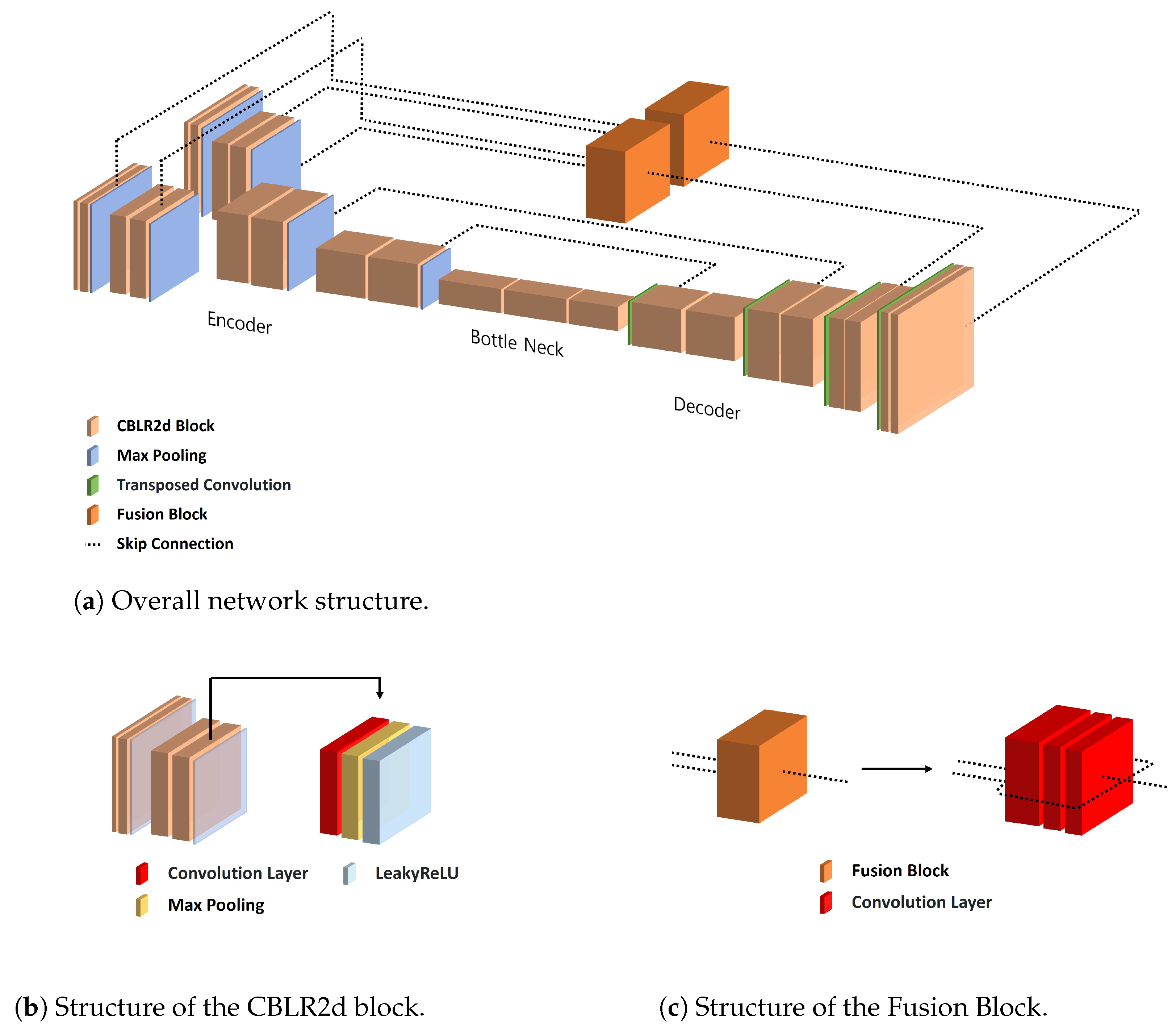
Architecture of R-Depth Net. (a) The defocussed Image and Optical Flow are processed by separate encoders, followed by a Fusion Block and a decoder to generate the Depth Map. (b) Structure of the CBLR2d block used in both encoder and decoder, consisting of Convolution, Batch Normalization, and Leaky ReLU. (c) Structure of the Fusion Block that resizes and concatenates the outputs of both encoders before passing to the decoder.
Figure 6.
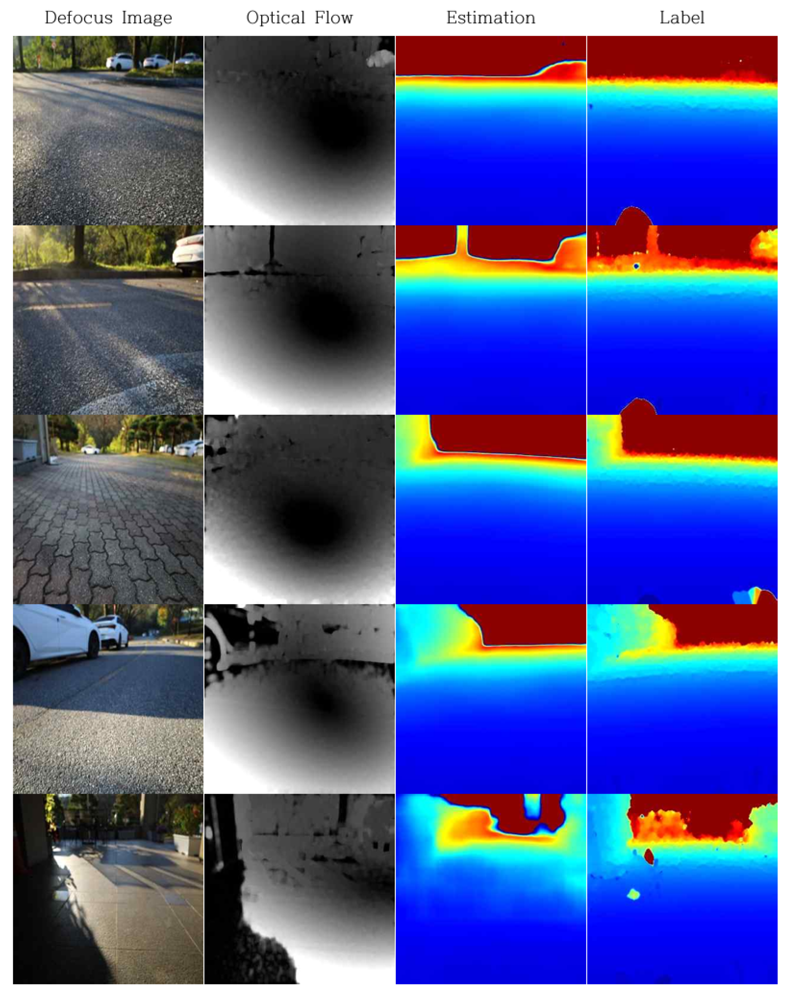
Training Result (Column 1: input Defocussed image, Column 2: optical flow magnitude (lighter: larger pixel displacement, darker: smaller pixel displacement), Column 3: estimation depth map (blue = near, yellow/green = intermediate, red = far), Column 4: label depth map (blue = near, yellow/green = intermediate, red = far)).
Figure 7.
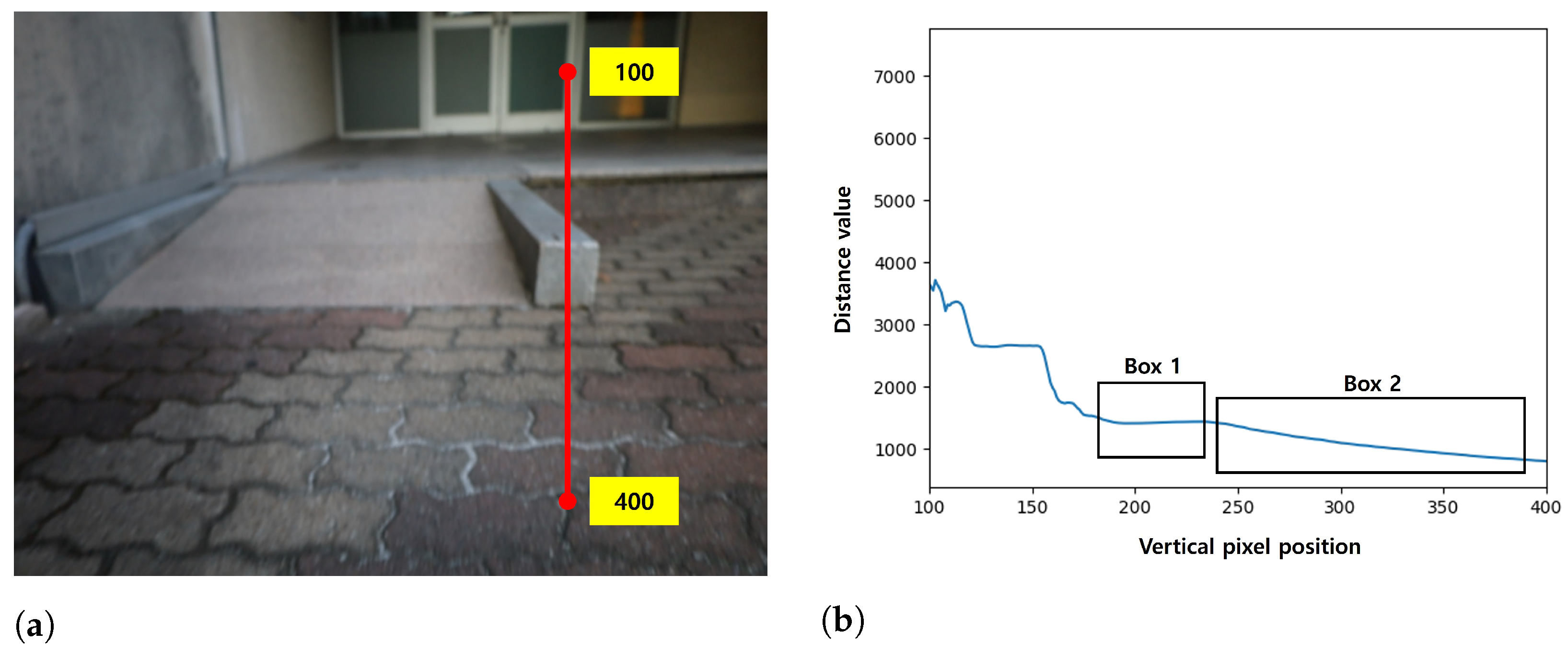
Depth variation profile for obstacle detection. (a) Sample Column Representing Depth. (b) Depth Profile with Box 1 Representing the Obstacle and Box 2 Representing the Ground (Horizontal Axis: Pixel Coordinates, Vertical Axis: Depth).
Figure 7.
Depth variation profile for obstacle detection. (a) Sample Column Representing Depth. (b) Depth Profile with Box 1 Representing the Obstacle and Box 2 Representing the Ground (Horizontal Axis: Pixel Coordinates, Vertical Axis: Depth).
Figure 8.
Example of a V-Disparity Map.
Figure 8.
Example of a V-Disparity Map.
Figure 9.
Example of Ground Mask.
Figure 9.
Example of Ground Mask.
Figure 10.
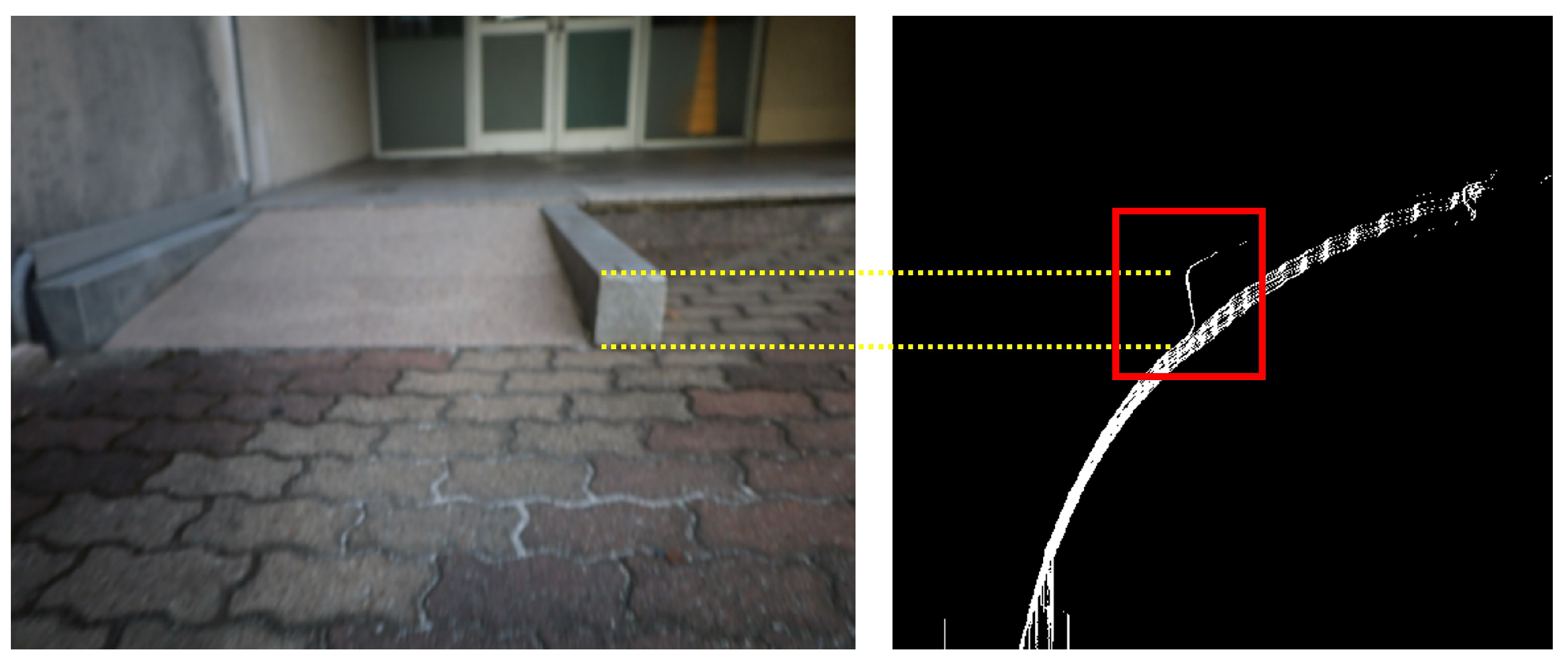
Detection of obstacle regions using the V-Disparity map.
Figure 10.
Detection of obstacle regions using the V-Disparity map.
Figure 11.
Relationship Between Camera and Obstacles for Height Calculation.
Figure 11.
Relationship Between Camera and Obstacles for Height Calculation.
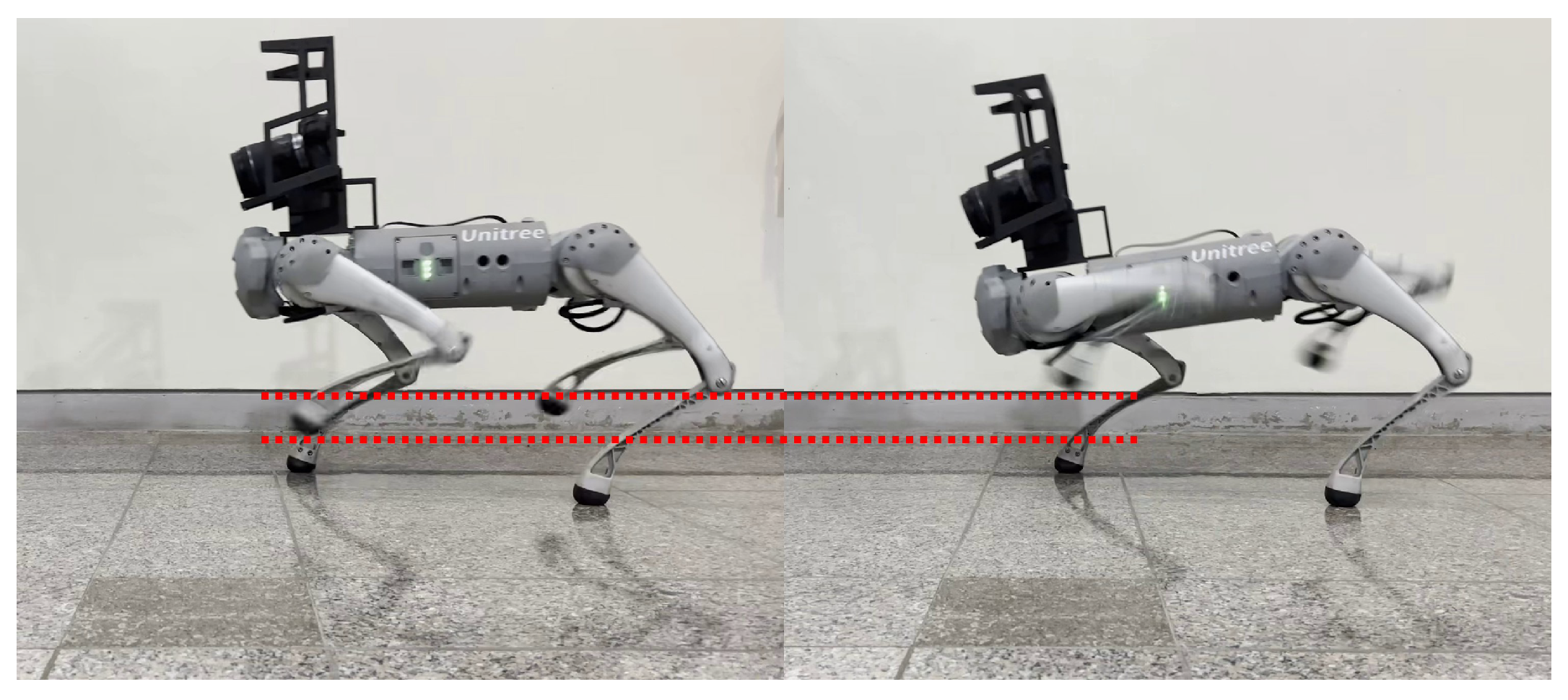
Figure 12.
Unitree Go1 Walking Mode (Left: Normal Walking Mode, Right: Obstacle Overcoming Mode). The red dashed line highlights the increased foot clearance in obstacle-overcoming mode.
Figure 12.
Unitree Go1 Walking Mode (Left: Normal Walking Mode, Right: Obstacle Overcoming Mode). The red dashed line highlights the increased foot clearance in obstacle-overcoming mode.
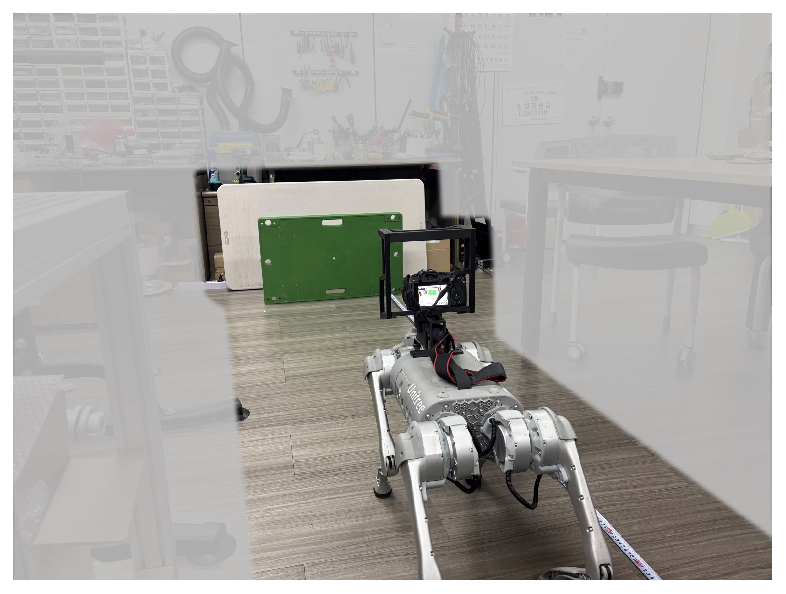
Figure 13.
Experimental Environment for Obstacle Distance Estimation Accuracy.
Figure 13.
Experimental Environment for Obstacle Distance Estimation Accuracy.
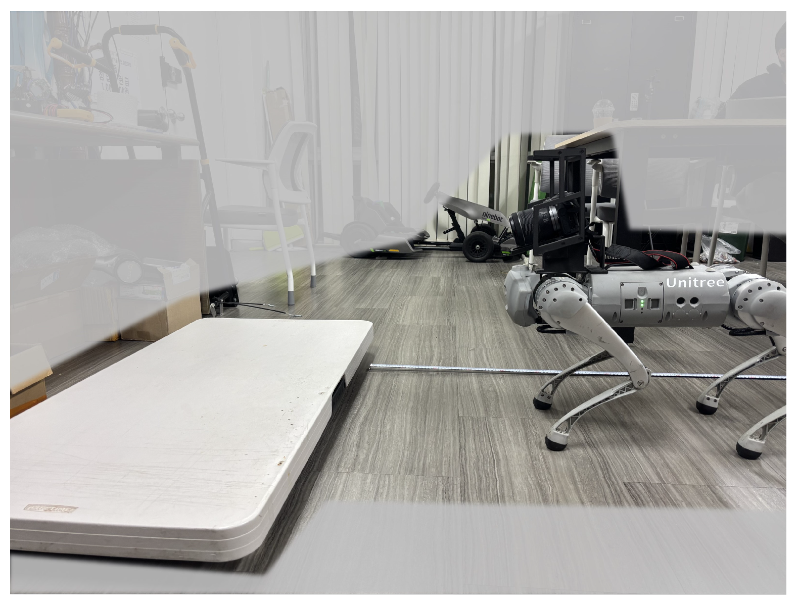
Figure 14.
Experimental Environment for Obstacle Height Estimation Accuracy.
Figure 14.
Experimental Environment for Obstacle Height Estimation Accuracy.
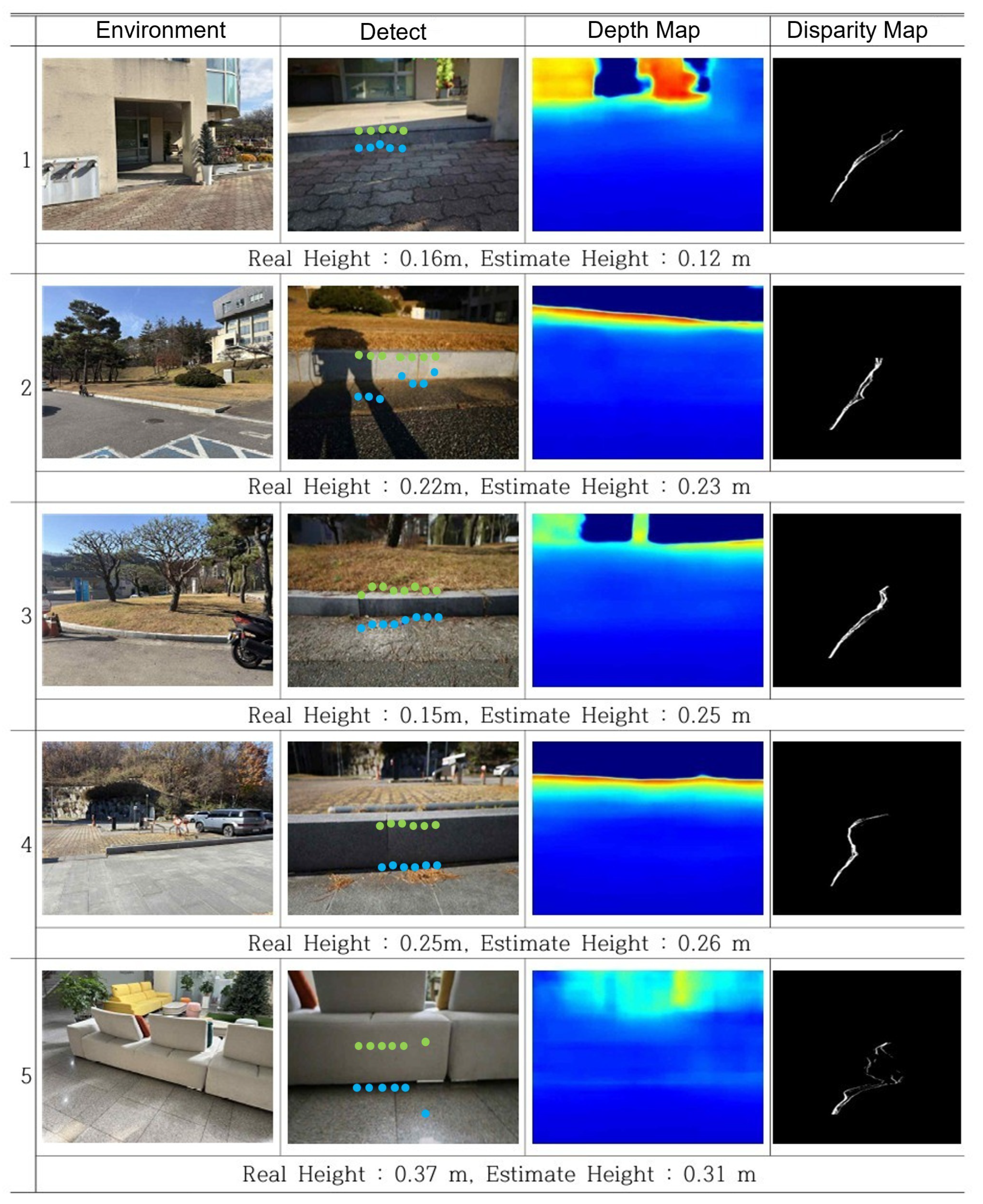
Figure 15.
Obstacle Height Estimation in Real-World Environments. (Column 2: Green dot indicates the obstacle top, and blue dot indicates the obstacle bottom. Column 3: blue = near, yellow/green = intermediate, red = far).
Figure 15.
Obstacle Height Estimation in Real-World Environments. (Column 2: Green dot indicates the obstacle top, and blue dot indicates the obstacle bottom. Column 3: blue = near, yellow/green = intermediate, red = far).
Figure 16.
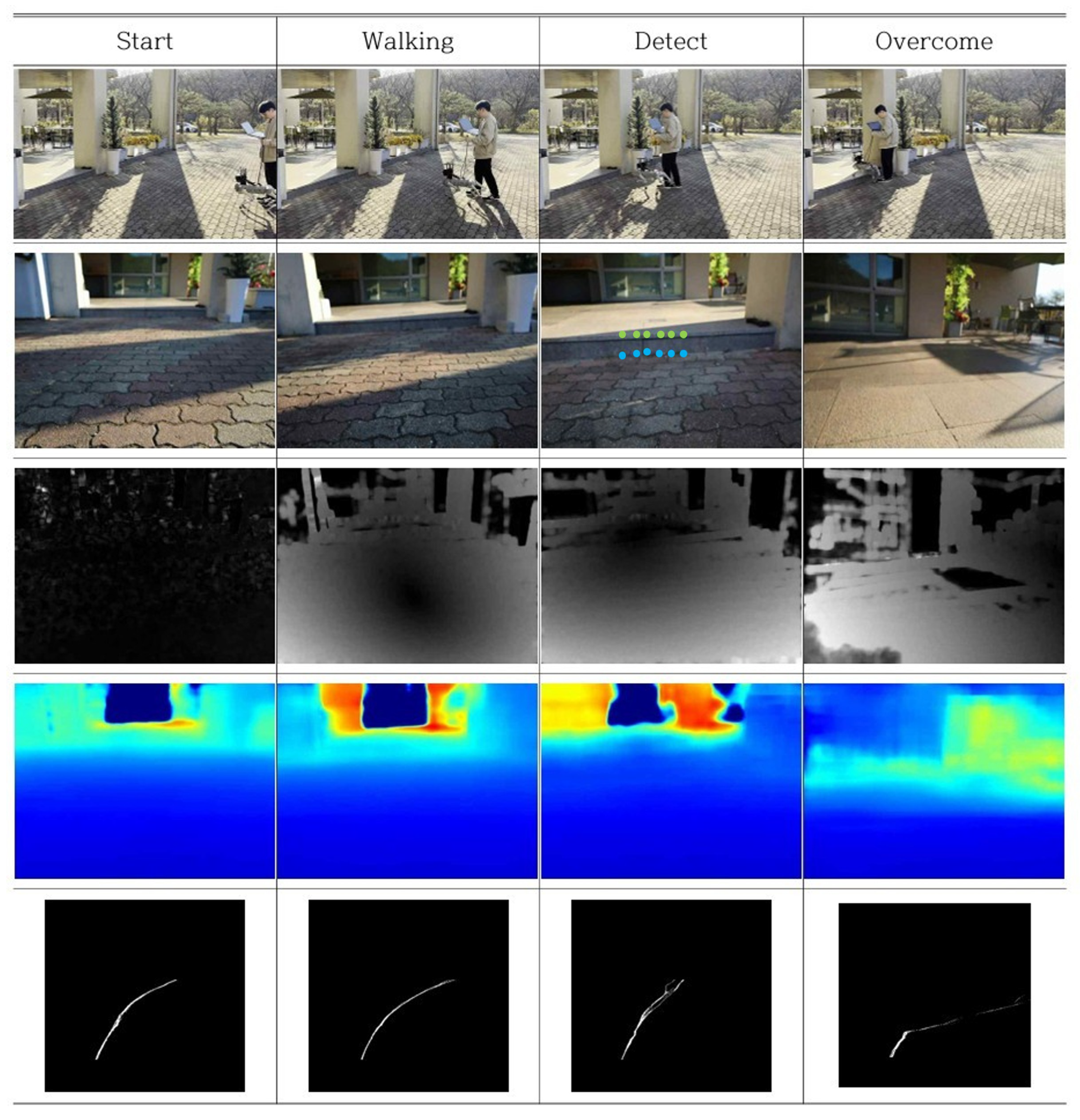
Obstacle Detection and Overcome Mode Transition in Real-World Environments (row 1: Experimental Environment, row 2: Robot View (Green dot indicates the obstacle top, and blue dot indicates the obstacle bottom), row 3: Optical Flow, row 4: Predicted Depth Map (blue = near, yellow/green = intermediate, red = far), row 5: V-Disparity Map).
Figure 17.
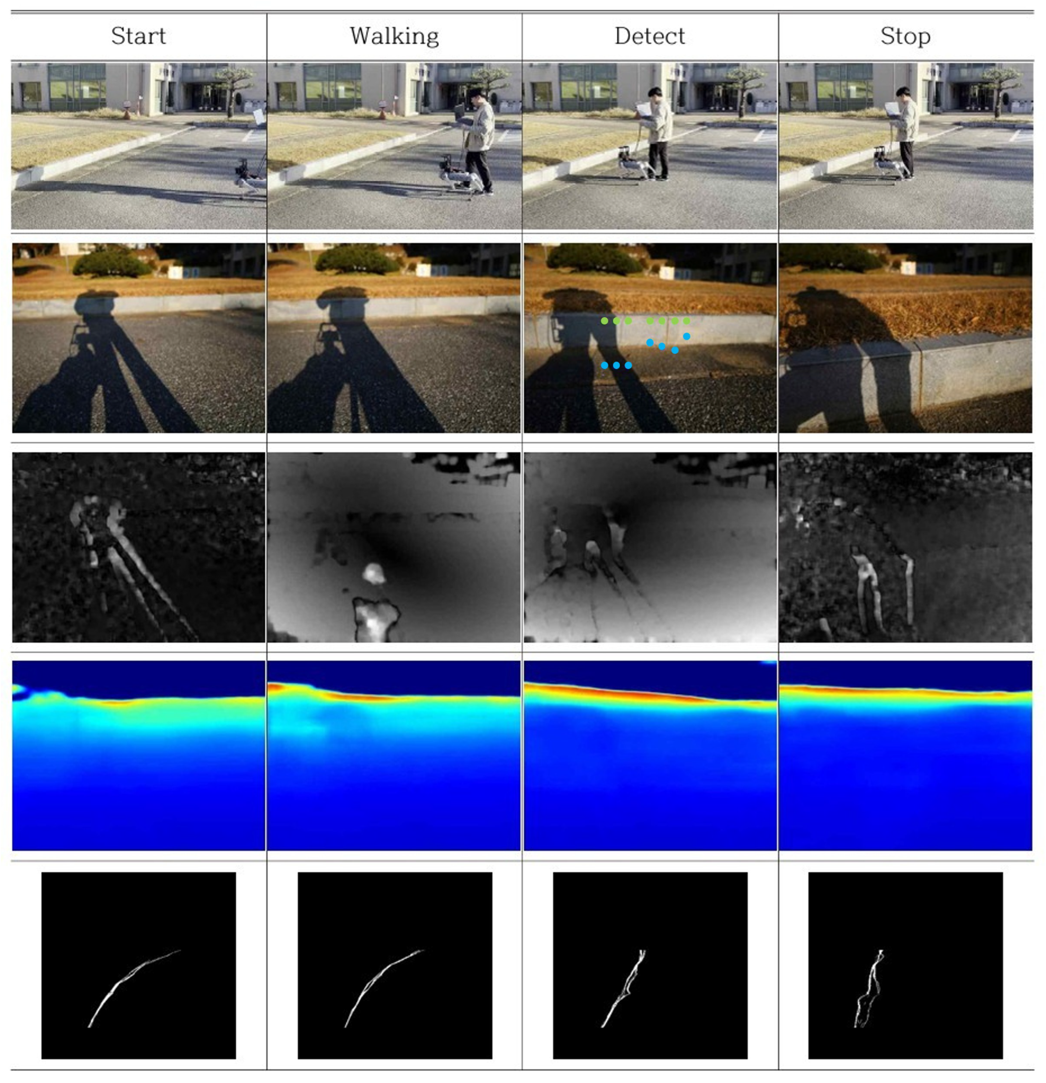
Obstacle Detection and Stop Mode Transition in Real-World Environments (row 1: Experimental Environment, row 2: Robot View (Green dot indicates the obstacle top, and blue dot indicates the obstacle bottom), row 3: Optical Flow, row 4: Predicted Depth Map (blue = near, yellow/green = intermediate, red = far), row 5: V-Disparity Map).
Table 1.
Variables Used to Calculate the degree of blur.
Table 1.
Variables Used to Calculate the degree of blur.
| Symbol | Meaning |
|---|
| s | Distance between lens and image sensor (mm) |
| f | Focal length (mm) |
| i | Distance between lens and image plane (mm) |
| b | Amount of blur (pixel) |
| o | Distance between lens and object (m) |
| D | Aperture diameter (mm) |
Table 2.
Training Result— Accuracy.
Table 2.
Training Result— Accuracy.
| Metric | Value |
|---|
| 95% |
| 97% |
| 98% |
Table 3.
Training Result—Error.
Table 3.
Training Result—Error.
| Metric | Value |
|---|
| Absolute Relative Error (AbsRel) | 6.5% |
| Squared Relative Error (SqRel) | 6.2% |
Table 4.
Impact of Depth from Defocus and Optical Flow on Test Dataset.
Table 4.
Impact of Depth from Defocus and Optical Flow on Test Dataset.
| Method | AbsRel (%) | SqRel (%) |
|---|
| No Defocus | 6.8 | 1.3 |
| Defocus | 2.9 | 5 |
| Defocus + Optical Flow | 2.4 | 4 |
Table 5.
Distance Estimation Error of R-Depth Net (absolute and percentage).
Table 5.
Distance Estimation Error of R-Depth Net (absolute and percentage).
| Distance | RMSE (m) | RMSE (%) | MAE (m) | MAE (%) |
|---|
| 3.0 m | 0.45 | 15.0 | 0.45 | 15.0 |
| 2.5 m | 0.06 | 2.4 | 0.05 | 2.0 |
| 2.0 m | 0.20 | 10.0 | 0.20 | 10.0 |
| 1.5 m | 0.29 | 19.3 | 0.29 | 19.3 |
| 1.0 m | 0.32 | 32.0 | 0.32 | 32.0 |
| Average | 0.30 | 15.7 | 0.26 | 15.7 |
Table 6.
Obstacle Height Estimation Error (absolute and percentage).
Table 6.
Obstacle Height Estimation Error (absolute and percentage).
| Obstacle Height | RMSE [m] | RMSE [%] | MAE [m] | MAE [%] |
|---|
| 0.10 m | 0.030 | 30.0 | 0.029 | 29.0 |
| 0.15 m | 0.039 | 26.0 | 0.035 | 23.3 |
| 0.20 m | 0.064 | 32.0 | 0.054 | 27.0 |
| Average | 0.048 | 29.3 | 0.040 | 26.4 |
