Long-Term Trends in Air Pollution in Poland on Selected Examples—A Spatial and Temporal Analysis of PM10 Concentrations

Abstract

The aim of this study was to analyze long-term trends and spatial variability of PM10 concentrations in Poland during the period 2019–2024, based on data from the European Air Quality Monitoring System (EAQ). The analysis covered nine locations representing three types of areas: large agglomerations (Warsaw, Kraków, Katowice), medium-sized cities (Wrocław, Poznań), and spa towns (Ciechocinek, Lądek-Zdrój, Świnoujście). An integrated statistical approach was applied, including Welch’s ANOVA, Linear Mixed Models (LMM), Generalized Additive Models (GAM), and Quantile Regression (FDR–BH). Mean PM10 concentrations in the analyzed period ranged from 17.43 µg/m³ in Świnoujście to 31.16 µg/m³ in Kraków, with 30.17 µg/m³ in Katowice and 27.90 µg/m³ in Warsaw. The largest differences between locations were observed during smog episodes —the 90th percentile values reached 56.61 µg/m³ in Kraków, 49.99 µg/m³ in Katowice, and 29.19 µg/m³ in Świnoujście. In most locations, a downward trend in PM10 levels was recorded over time; however, regional differences persist. The GAMs confirmed strong seasonality (winter maximum, summer minimum), while quantile regression indicated that the highest risk of smog episodes occurs in southern Poland. The novelty of this study lies in the integration of three complementary modeling approaches (LMM, GAM, and Quantile Regression) in the analysis of the spatio-temporal variability of PM10, as well as in the innovative comparison-unique in the literature-of agglomerations, medium-sized cities, and spa towns in Poland based on a uniform, reference EAQ dataset. This approach made it possible to reveal persistent environmental disparities of significant relevance to the national anti-smog policy and enables a more realistic assessment of environmental risk within the European research context.

1. Introduction

Air pollution refers to the presence of harmful substances in the Earth’s atmosphere and constitutes a serious global problem. According to the European Council [1], approximately 300,000 people die prematurely each year due to air pollution. It also contributes to numerous respiratory and cardiovascular diseases.

Despite numerous studies on air quality in Europe, a significant research gap remains concerning long-term spatial analyses of pollution at the national scale using uniform measurement data. Previous research has mainly focused on individual agglomerations or industrial areas [2,3,4], short-term analyses of pollution episodes [5,6,7], or modeling of pollutant transport without direct reference to monitoring data [8,9,10]. However, no systematic comparison has been identified regarding regional differences in PM10 levels in Poland, taking into account various types of locations (agglomerations, medium-sized cities, and spa towns) as well as long-term temporal trends. Moreover, although the European Air Quality Assessment system provides consistent and comparable measurement data, its potential has not yet been utilized for a comprehensive spatio-temporal analysis of PM10 concentrations in Poland. The present study aims to fill this research gap.

The analytical methods applied in this study were selected to ensure their applicability not only in the context of Polish cities but also in other locations with diverse environmental conditions. As a result, the proposed research approach can be replicated and adapted to different local contexts, enabling comparisons at both national and international levels. The findings obtained are therefore of a universal character and may serve as a foundation for further research as well as for shaping environmental policies in other regions.

2. Literature Review and Definition of the Research Problem

Effective air quality management relies on precise measurement and environmental monitoring. The European Air Quality Index (EAQ) provides information on air quality within the EU, based on 2000 air monitoring stations in Europe, which collect hourly information on the concentrations of most harmful air pollutants [3,5,11,12,13]. In Poland, air pollution monitoring is carried out by the Chief Inspectorate of Environmental Protection, which operates under the European Air Quality Index. Apart from precise measurement in air quality management, the analysis of the obtained results is also essential. There are a number of methods for environmental data analysis. Edupuganti et al. [11] developed sensor nodes connected with a GPS system for data storage, then used the IoT method and published the results online in the public domain. Mohan et al. [14], with the aim of improving environmental measurement analysis, presented a three-stage system of air pollution monitoring, with the data stored in a public cloud. Iman et al. [15] demonstrated the high effectiveness of machine learning (ML) algorithms in predicting air quality. The authors examined four classical algorithms: support vector classifier, random forest classifier, logistic regression, and decision tree classifier. Ghosh et al. [16] analyzed environmental data using mathematical modeling to assess air quality. The proposed method achieved an effectiveness level of 79%. Calvile et al. [17] used mathematical techniques to analyze long-term trends in pollutants such as PM₁₀, NO, NO₂ and O₃, in order to estimate the impact of the introduction of new vehicle technologies on the final air quality in Greece. In the study by Giechaskiel et al. [18], trends in air pollution and meteorological parameters were analyzed in order to present long-term forecasts of air quality. In [19,20], trends in annual observations of PM₁₀ and their impact on health in Iran were examined. An increasing trend in mean annual PM₁₀ concentrations and a corresponding rise in disease incidence, particularly among children under three years of age, was noted. The authors of [21] used mathematical models to compare air quality trends for selected countries. Sondej et al. [22] monitored and analyzed SO₂ and NO₂ pollution in a protected area in Poland. The authors also compared the results with EU averages. During the six-year observation period, a clear decline in SO₂ levels was observed in the protected area, while NO₂ concentrations decreased only slightly, in line with observations across the EU [23,24].

It is worth noting that although the European Environment Agency and national environmental monitoring institutions regularly publish reports on air quality and long-term changes in particulate matter concentrations in Europe [25,26], these analyses are aggregated in nature and focus mainly on the national or community level. However, there is a lack of detailed spatio-temporal analyses for Poland that would use the uniform measurement data system of the European Air Quality network while simultaneously accounting for the diversity of area types (agglomerations, medium-sized cities, and spa towns). In addition, no studies have been identified that simultaneously analyze mean values, seasonal trends, and high-concentration episodes (P90) based on an advanced modeling approach enabling the separation of temporal and spatial variability.

In view of the above, two research questions were posed in this article. How are long-term air quality trends, using PM₁₀ as an example in Poland, shaped on the basis of EAQ data for an EU member state, with particular emphasis on the recent years (2019–2024)? And do disparities exist in the development of PM₁₀ concentrations for different areas of Poland, taking into account both highly populated urban agglomerations and towns with health resort status?

3. Materials and Methods

In order to answer the above research questions, an analysis of long-term trends in selected air pollutants (PM₁₀) in Poland (2019–2024) was carried out on the example of selected cities, and large urban agglomerations were compared with smaller cities and towns recognized as health resorts. The scope of the data included air quality measurement data obtained from the Measurement Data Bank of the Chief Inspectorate of Environmental Protection, which operates under the EAQ [23,27]. A total of nine locations were analyzed, including large agglomerations such as Warsaw, Kraków, and Katowice; medium-sized cities such as Wrocław and Poznań; and small towns—Ciechocinek, Lądek-Zdrój, and Świnoujście, recognized as health resorts. The measurement data were obtained from the European Air Quality (EAQ) system, which includes publicly available measurements conducted by the Chief Inspectorate of Environmental Protection (GIOS). The analysis covered the period 2019–2024, adopted as a range enabling the assessment of current air quality trends following the implementation of key anti-smog policy instruments in Poland (anti-smog resolutions and the “Clean Air” program). In the relevant literature, a period of ≥5 years is considered sufficient for evaluating air quality trends in environmental analyses [16,25,28,29].

In each location, one representative monitoring station was analyzed to avoid local distortion of results caused by linear (traffic) or point-source emissions. The selection of stations complies with EU reference criteria. The applied monitoring stations included both automatic and manual measurement methods. Station codes are shown in

Table 1. Chief Inspector of Environmental Protection station codes.

Location	Station Code
Kraków	PL0039A
Katowice	PL0008A
Warszawa	PL0308A
Poznań	PL0572A
Wrocław	PL0193A
Gdańsk	PL0775A
Ciechocinek	PL0066A
Lądek-Zdrój	PL0504A
Świnoujście	PL0862A

.

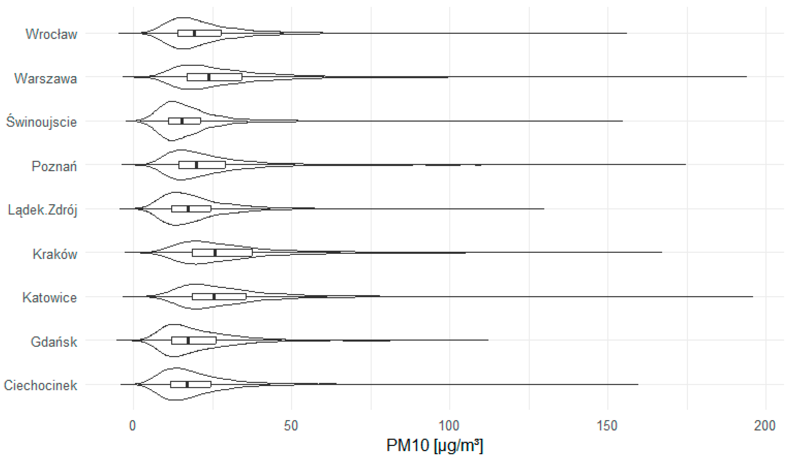
At the stage of exploratory data analysis (EDA) [30,31], a set of visualizations was prepared. First, the distributions of concentrations in individual locations were visualized—using violin plots and boxplots, which made it possible to assess simultaneously the shape of the distribution, the median, and the dispersion of the data (Figure 1). The mean values and 90th percentile are also presented in

Table 2. Summary of global tests assessing the impact of location on PM₁₀ concentration.

Test	Statistic	p-Value
ANOVA (classical)	F(8, 19,719) = 310.63	<$1{·10}^{-4}$
Omega2 (overall effect)	${\omega }^2$ = 0.11 [0.1, 1]	NA
Permutation test (Fisher–Pitman)	${\chi }^2$ = 2207.8	<$1{·10}^{-4}$

. The analyses were performed in the R environment, version 4.2.2 producer: R-project. The symbol used in Table 2 omega square is ${\omega }^2$.

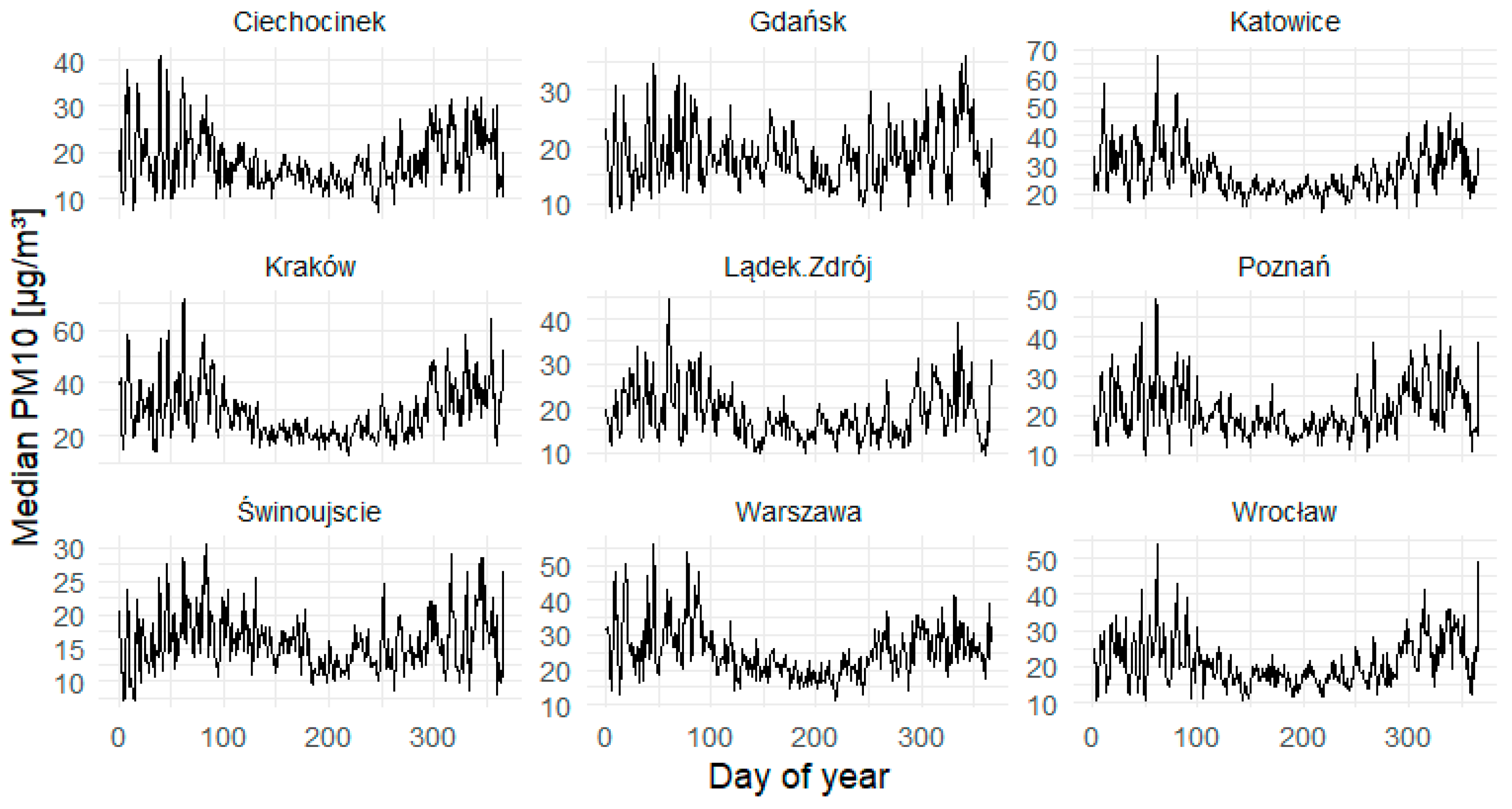
Next, by first assessing daily seasonality, the medians of PM₁₀ concentrations for each day of the year were calculated and presented in the form of trend curves for individual locations, which made it possible to identify cyclical seasonal patterns. Daily seasonality is presented in Figure 2, daily graphs will allow for the assessment of the median and dispersion over the observed years.

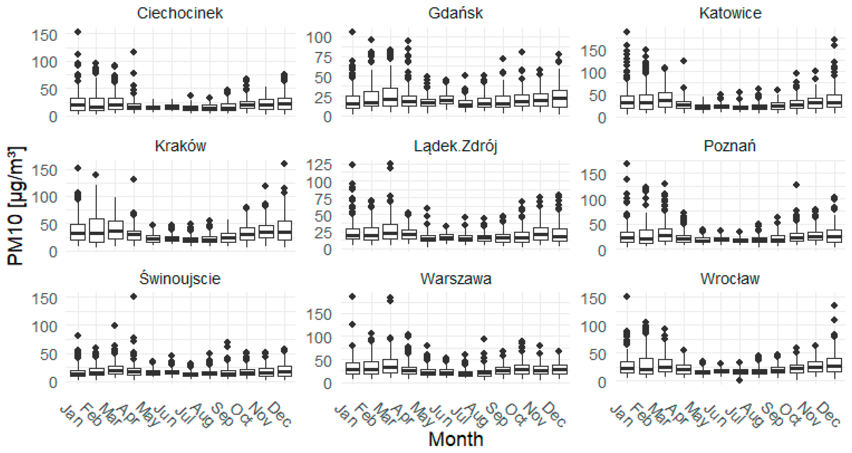
Monthly seasonality was then presented in the form of boxplots divided by months and locations, which made it possible to compare variability on a monthly scale (Figure 3). Figure 3 will allow for a comparison of medians and dispersion with daily graphs over the observed years.

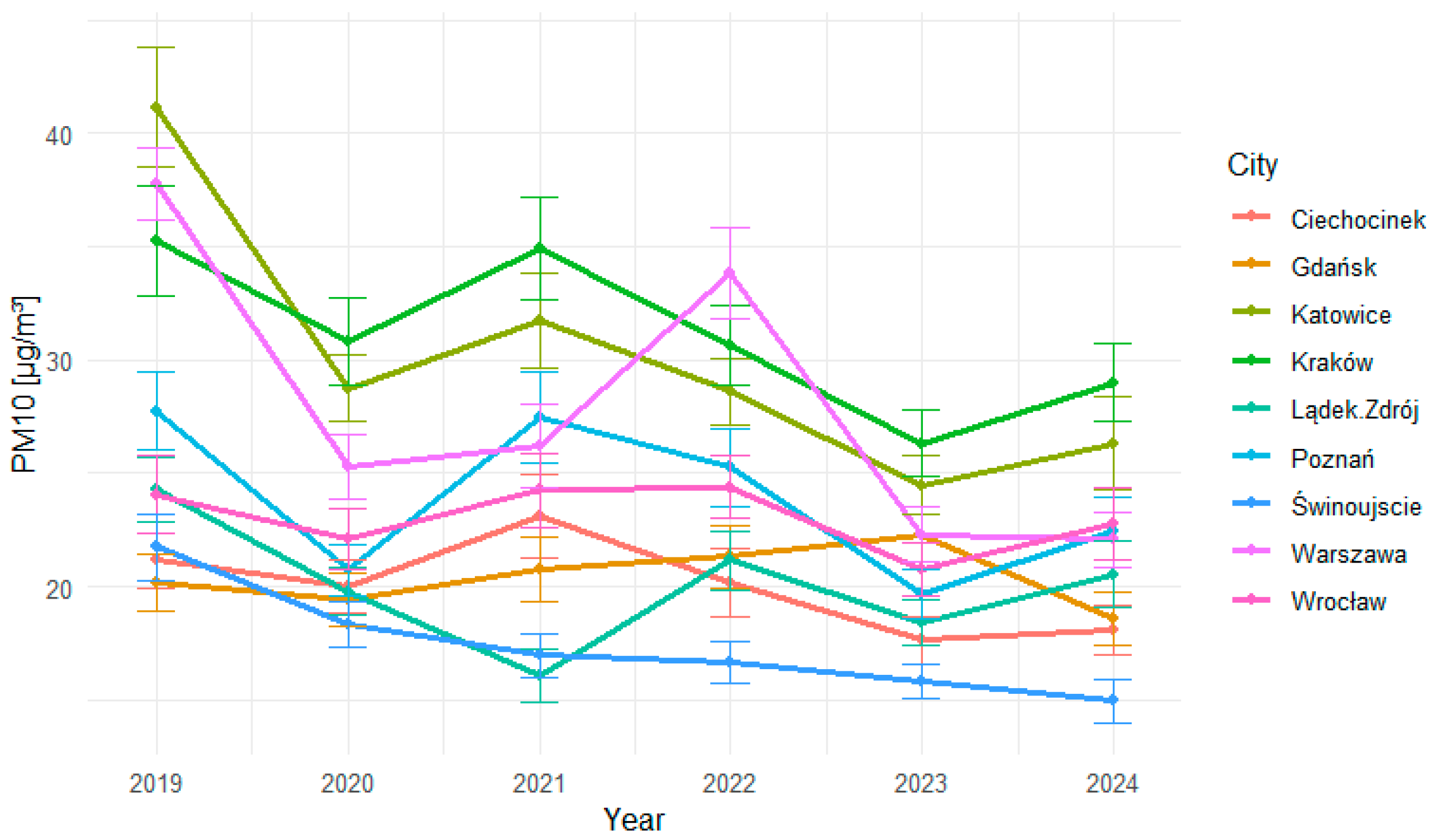
For the purpose of a preliminary visualization of the analyzed time series, annual means and calculated 95% confidence intervals were also presented (Figure 4).

In all locations, a clear daily seasonality within the annual cycle can be observed—PM₁₀ concentrations are highest in winter (at the beginning and end of the year) and lower during the summer period. The most pronounced seasonal fluctuations are observed in cities with high levels of traffic-related and/or heating-related pollution (e.g., Katowice, Kraków, Warsaw). Health resort or coastal locations (Świnoujście, Lądek-Zdrój) are characterized by lower median values and smaller seasonal amplitudes. The monthly boxplots confirm the observations from the daily plots: in the winter months (January, February, December), both the median and the dispersion of values are significantly higher than during the summer period. In Kraków and Katowice, particularly high variability is visible in winter—the presence of numerous outliers indicates frequent episodes of elevated concentrations. In summer, values are more stable and lower across all locations, confirming the seasonal nature of the problem. Data analysis shows a significant decline followed by an increase in 2020. This phenomenon can be explained by the COVID pandemic, where a significant reduction in transport and industry contributed to a decrease in air pollution. However, over the observed years 2019–2024, a general downward trend in annual mean PM10 concentrations is visible in most locations. The highest levels persist in agglomerations with heavy traffic and emissions from individual heating systems (Kraków, Katowice, Warsaw). Coastal and spa towns (Świnoujście, Ciechocinek) show significantly lower annual mean concentrations, usually below 25 µg/m³. The confidence intervals indicate moderate estimation uncertainty but do not alter the main conclusion regarding the improvement of air quality over time.

3.1. Statistical Testing of Differences

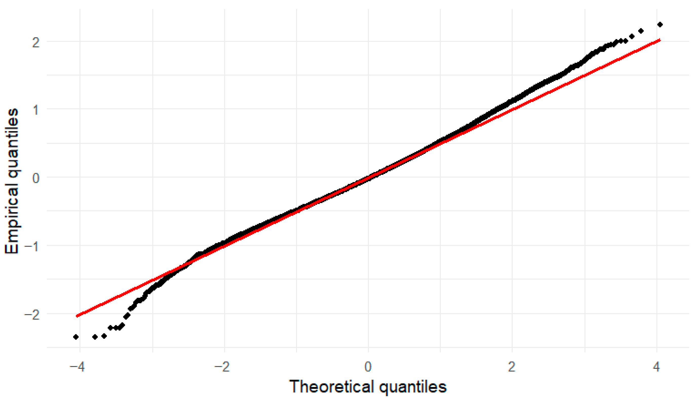
Due to the right-skewness and heteroskedasticity of the data, a logarithmic transformation log(x + 1) was applied, which is a recommended procedure for variance stabilization in environmental analyses. The adequacy of the transformation was assessed using the Breusch–Pagan test, comparing the stability of variance before and after transformation, as well as graphical residual diagnostics (QQ-plot). All analyses were performed on the transformed data. Since the assumptions of normality and homoscedasticity are rarely fully met in environmental datasets, variance stabilization through logarithmic transformation, combined with robust model diagnostics, is considered acceptable and widely recommended in the literature [32,33,34].

The Breusch–Pagan test confirmed a significant reduction in heteroskedasticity after the log(x + 1) transformation (BP = 225.5, p < 0.001 before transformation; BP = 27.68, p < 0.001 after transformation), which justifies the application of the transformation in subsequent modeling.

The normality of the residual distribution was assessed using the QQ-plot (Figure 5). The residual distribution after the log(x + 1) transformation was sufficiently close to normal for the purposes of statistical modeling. According to the Central Limit Theorem, for large samples, the approximate normality of the mean distribution is ensured, which justifies the use of linear regression–based methods and allows for valid statistical inference.

To compare mean concentration levels between locations, several complementary methods were employed: (i) Welch’s ANOVA, which is robust to variance heterogeneity, (ii) the effect size measure Omega squared (ω²), which indicates the proportion of variance explained by the factor, and (iii) the Fisher–Pitman permutation test, a non-parametric counterpart of ANOVA, testing the null hypothesis of identical distributions across all groups. Given the numerous pairwise comparisons between locations, false discovery rate (FDR) control was applied using the Benjamini–Hochberg (BH) method. This approach reduces the risk of Type I errors across a series of tests, while maintaining greater statistical power than the classical Bonferroni correction. Results marked as significant should therefore be interpreted as statistically reliable differences under the assumed FDR level (q < 0.05).

Global analyses demonstrated a significant effect of location on PM10 concentration levels (Table 2). Welch’s ANOVA, conducted on logarithmically transformed data, confirmed significant differences between groups (F(8, 8216) = 316.85, p < 0.0001). The overall effect size was estimated at ω² = 0.11 (95% CI: 0.10–1.00), indicating that approximately 11% of the variability in PM10 concentrations can be attributed to differences between locations. Similarly, the non-parametric Fisher–Pitman permutation test also unequivocally confirmed significant differences in the distributions across groups (χ² = 2207.8, p < 0.0001). These results consistently indicate that spatial factors play an important role in shaping PM₁₀ concentration levels.

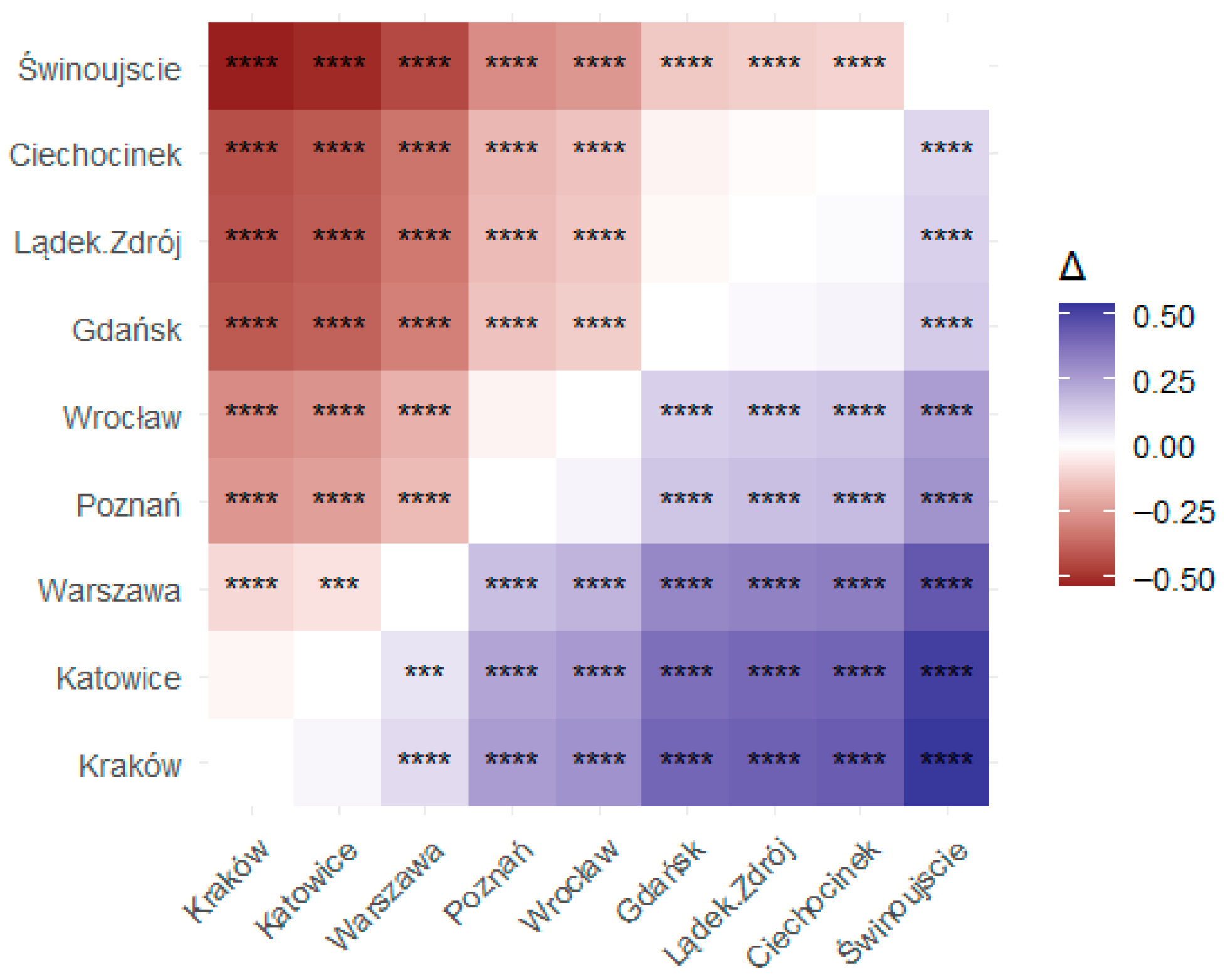
Subsequently, post hoc comparisons were performed using the Games–Howell test, which is robust to unequal variances and group sizes. The results are presented in Figure 6. The * symbol in Figure 6 indicates levels of statistical significance. In practice, it indicates how significant the difference between two groups is in a multiple comparison. The scale ranges from one * to ****.

Post hoc Games–Howell tests revealed significant differences between most locations. The highest mean concentrations (after log transformation) were observed in Kraków and Katowice, significantly higher than in Świnoujście (Δ ≈ 0.5, p < 0.001). Ciechocinek and Gdańsk did not differ from each other (p = 0.77). Similarly, no differences were found between Katowice and Kraków (p = 0.90) or between Poznań and Wrocław (p = 0.70). Świnoujście showed lower values than most locations, while Warsaw occupied an intermediate position.

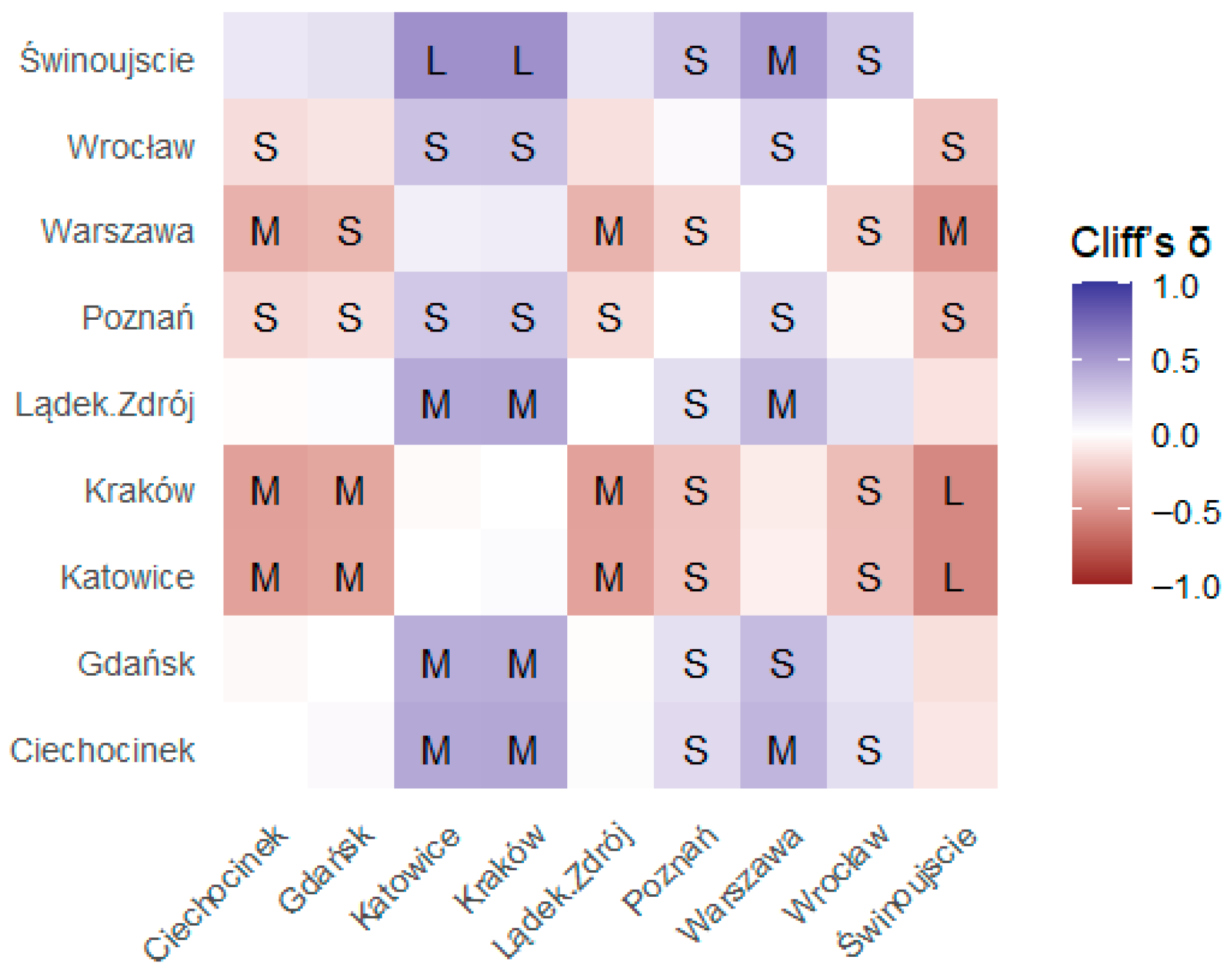
To complement the significance tests, non-parametric effect sizes for pairwise comparisons of locations were calculated using Cliff’s delta. This measure describes the probability that observations from one location exceed those from another. The interpretation followed the thresholds: <0.147—negligible, 0.147–0.33—small, 0.33–0.474—medium, ≥0.474—large effect.

The analysis of effect sizes indicated that many differences between locations (δ < 0 indicates that the second location has higher values), although statistically significant, had limited practical importance (δ in the range of 0.15–0.30). Medium differences were observed, among others, between Kraków and Ciechocinek (δ = −0.43) and between Warsaw and Świnoujście (δ = 0.47). The strongest differences (δ ≈ 0.54, large effect) were found between Katowice and Świnoujście and between Kraków and Świnoujście, indicating clearly higher PM10 levels in the Silesian and Kraków agglomerations compared to the coastal town. The results are presented as a Cliff’s δ matrix (Figure 7), where color reflects the δ value (−1…1), letters (L/M/S) denote the effect size category, and asterisks indicate significance after BH correction.

3.2. Mathematical Modeling

In the further analysis, in addition to classical tests, three complementary modeling approaches were applied to capture more comprehensively the spatial and temporal variability of PM₁₀ concentrations [35]:

(1)

Linear mixed model (LMM) with a random day effect (1|date), which made it possible to “filter out” location-specific differences from common daily fluctuations (e.g., nationwide episodes). Location effect estimates were calculated on the logarithmically transformed scale and then back-transformed to µg/m³. This allowed for a comparison of marginal mean PM₁₀ values between locations while accounting for daily variability. Multiple pairwise contrasts were adjusted using the Benjamini–Hochberg (BH) method, ensuring control of the false discovery rate (FDR).

(2)

Generalized additive model (GAM), which incorporated both fixed differences between locations and nonlinear temporal patterns. A cyclic spline for the day of year was used to model annual seasonality, while long-term trends were captured through separate smooth functions for each location. This enabled the estimation of the extent to which the observed differences between locations resulted from distinct seasonal patterns and trends rather than from average PM₁₀ level differences alone. Significance tests and contrasts between locations were also corrected using the BH method (FDR).

(3)

Quantile regression, applied to the median (τ = 0.5) and the upper tail of the distribution (τ = 0.9), which enabled the analysis not only of typical PM₁₀ values but also of extreme smog episodes. Comparisons against the reference location (Ciechocinek) indicated which locations were characterized by higher or lower values both in the median and in the 90th percentile. In this way, a complementary picture of variability was obtained—encompassing average values, seasonality and trends (GAM), as well as extreme situations (quantile regression).

In this study, a set of complementary methods was deliberately applied to enable a multifaceted analysis of environmental data with a complex spatio-temporal structure. The use of a single statistical technique, such as a classical linear model, would be insufficient for an accurate interpretation of the observed phenomena. For this reason, a three-stage analytical framework was designed, consisting of:

• Analysis of differences between locations, in which the Welch ANOVA and Fisher–Pitman permutation tests were applied as global analyses, followed by post hoc Games–Howell tests supported by effect size measures (Cliff’s δ), allowing for differentiation of results in terms of both statistical and practical significance.
• Development of models accounting for data structure, specifically linear mixed models with a random effect of the measurement day, which made it possible to eliminate the influence of common, nationwide pollution episodes and thereby to reliably assess differences between locations without the risk of temporal pseudoreplication.
• Modeling of trends and seasonal variability, specifically flexible generalized additive models (GAM) and quantile regression, which enabled not only the identification of mean temporal trends but also the analysis of extreme values (τ = 0.9), crucial from the perspective of air quality management.

It should be emphasized that the selection of methods was guided by their suitability for analyzing environmental data characterized by non-normal distributions and heterogeneous variances, as well as by their capacity for transparent and application-oriented interpretation of results. All multiple comparison analyses were subjected to Type I error control using the Benjamini–Hochberg procedure, which further increased the reliability of the statistical inference.

3.2.1. Linear Mixed Model (LMM)

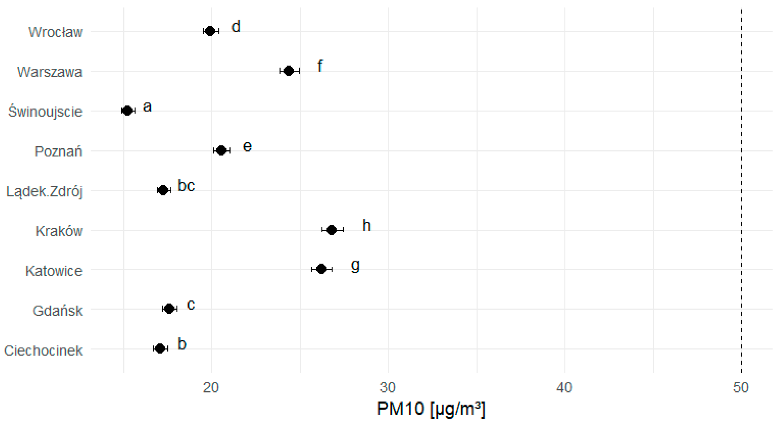
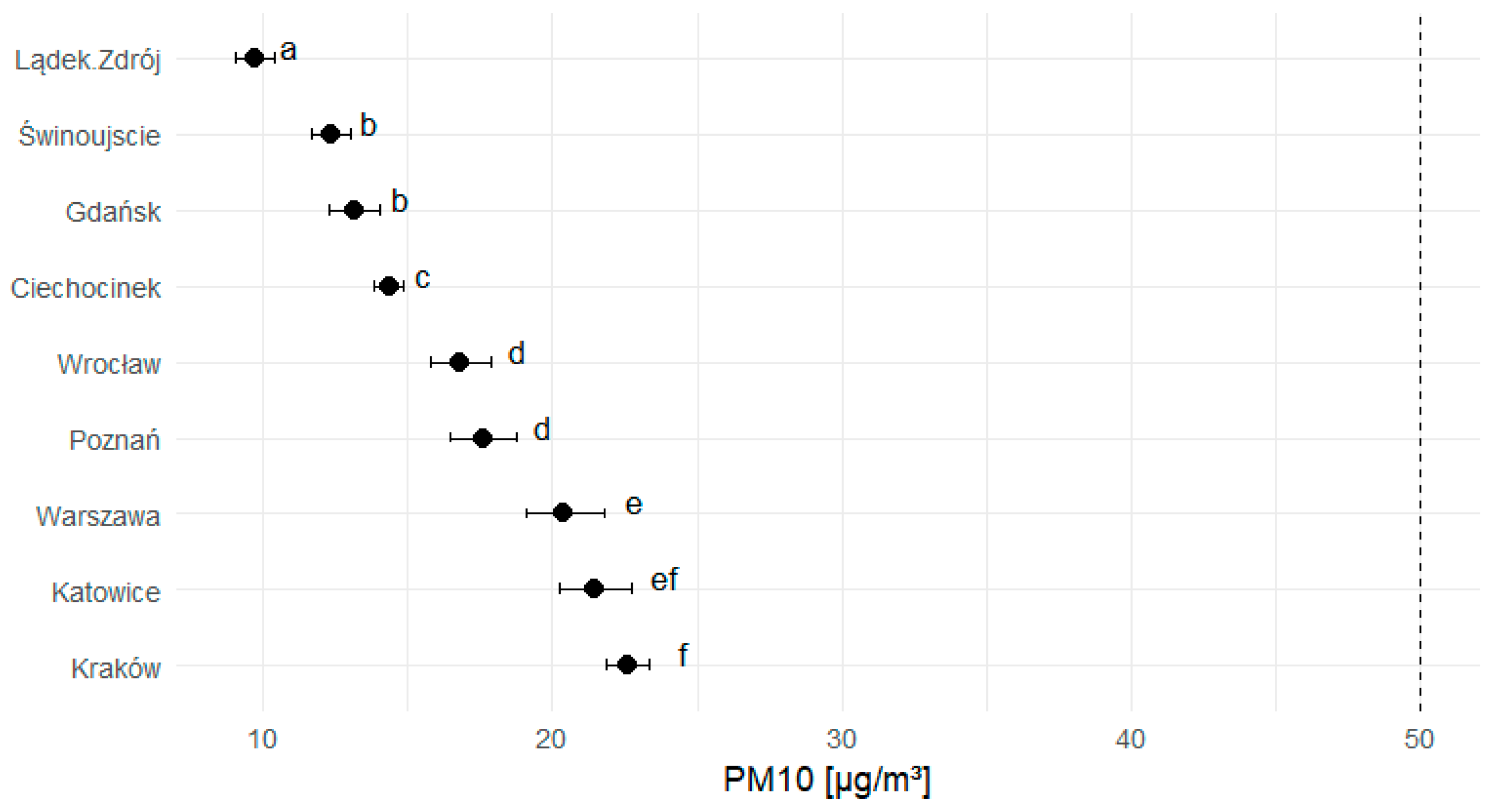
A linear mixed model with a random effect of the measurement day was estimated in the form: lpm ~ location + (1|date). This made it possible to compare locations while controlling for nationwide fluctuations. The model confirmed significant differences between locations (η² partial = 0.27, 95% CI: 0.26–1.00). Estimates were calculated on the log scale, and then comparisons and confidence intervals were back-transformed to µg/m³. The highest values on the log scale were recorded in Kraków and Katowice (β ≈ +0.42, corresponding to an increase of approx. 52% relative to the reference point), followed by Warsaw (+0.34 → +41%), Poznań (+0.17 → +19%), and Wrocław (+0.15 → +16%). Świnoujście was characterized by significantly lower values (β = –0.11 → –10%). Ciechocinek, Gdańsk, and Lądek-Zdrój showed similar levels, with no significant differences compared to the reference value.

Most pairwise comparisons were statistically significant after BH correction, except for the pairs Ciechocinek–Lądek-Zdrój, Gdańsk–Lądek-Zdrój, and Katowice–Kraków, where the differences were minimal. Figure 8 presents the marginal mean PM10 concentrations (µg/m³) estimated by the mixed model, along with 95% CIs (after back-transformation). Letters above the points indicate homogeneous groups: locations marked with the same letter do not differ significantly, while different letters indicate statistically significant differences. The dashed line marks the 50 µg/m³ threshold (the daily PM10 limit value according to EU/WHO standards [36]). The average PM10 concentration limits for individual locations are shown in Figure 8.

3.2.2. GAM

To capture seasonal effects and long-term trends, a generalized additive model (GAM) was fitted with a cyclic spline for day of year and separate smooth functions of time for each location. The model revealed clear seasonality (s(doy): edf = 17.33, F = 95.61, p < 0.001), consistent with the typical annual PM₁₀ cycle (winter maximum, summer minimum), as well as significant long-term trends in most locations (all p < 0.001). The complexity of the trends varied: in Kraków and Ciechocinek, the course was close to linear (edf ≈ 1), whereas in Warsaw, Gdańsk, Lądek-Zdrój, Poznań, Wrocław, and Świnoujście it was more complex (edf ~ 5–9). The model fit was moderate but significant for environmental data (R²adj = 0.233, deviance explained = 23.6%).

Parametric coefficients (reference point: Ciechocinek) indicated that Gdańsk (+0.027; p = 0.063) and Lądek-Zdrój (+0.010; p = 0.473) did not differ significantly, whereas Katowice (+0.409), Kraków (+0.430), Warsaw (+0.339), Poznań (+0.174), and Wrocław (+0.147) were significantly higher (all p < 0.001), while Świnoujście was significantly lower (−0.106; p < 0.001). The analysis of marginal means after GAM (emmeans, BH correction) showed that most of the 36 contrasts between locations were significant, with no significant differences observed, among others, for the pairs: Katowice–Kraków, Katowice–Warsaw, Poznań–Wrocław, and Gdańsk–Świnoujście. 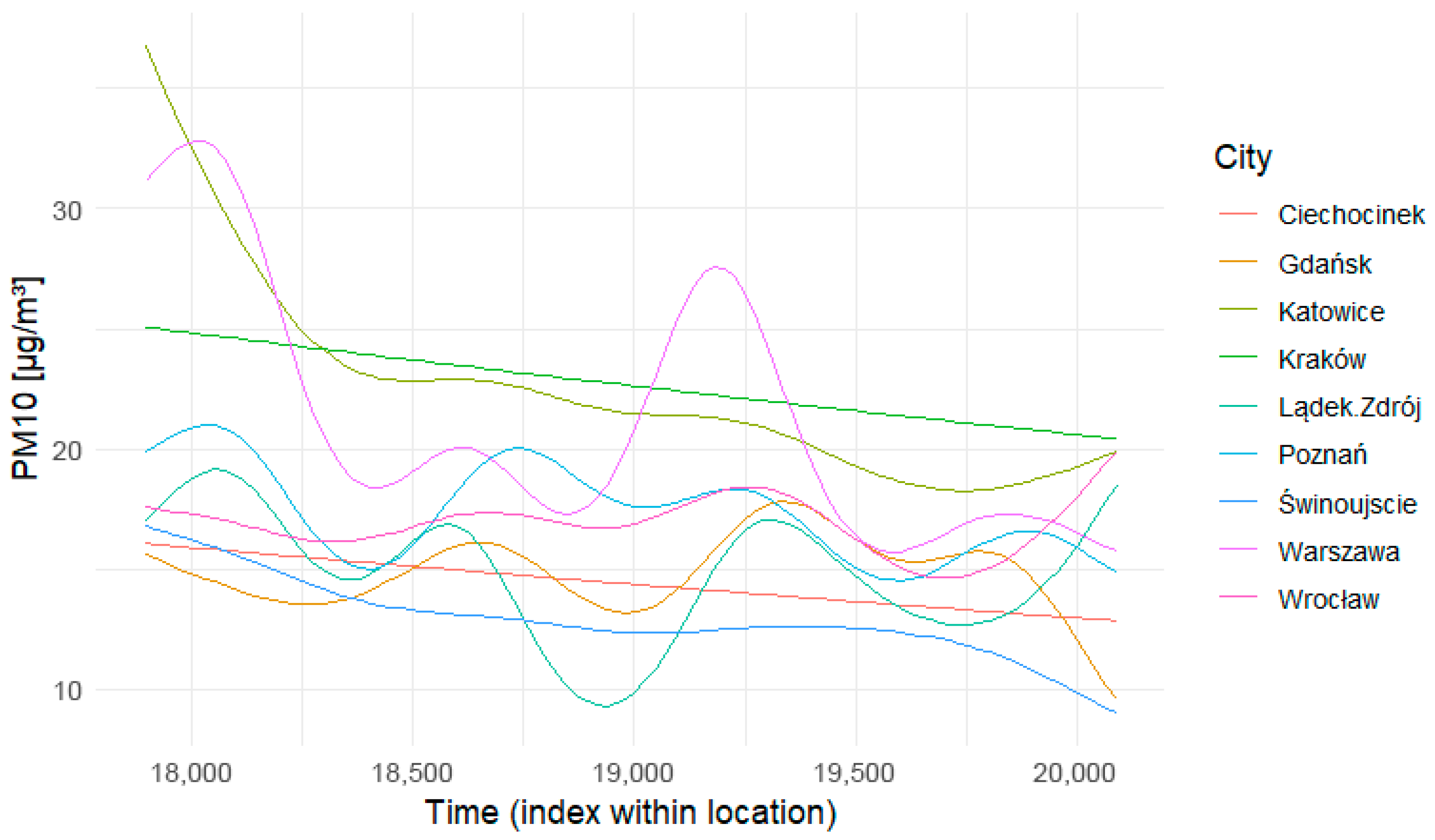Figure 9 presents the estimated seasonal PM₁₀ concentration patterns for individual locations.

Figure 10 presents the marginal mean PM₁₀ values after controlling for seasonality and long-term trends, together with confidence intervals. Letters above the points indicate homogeneous groups.

The GAMs revealed clear differences in both seasonality and long-term trends of PM₁₀ concentrations among the analyzed locations. In all cities, a recurring annual cycle with a winter maximum and a summer minimum was observed (p < 0.0001 for the s(doy) effect); however, the amplitude of seasonality varied substantially across regions. The highest seasonal variability was recorded in southern agglomerations (Kraków, Katowice), where differences between winter and summer values reached 25–35 µg/m³, while in medium-sized cities (Poznań, Wrocław) the amplitude ranged between 15 and 18 µg/m³, and in spa towns (Ciechocinek, Świnoujście, Lądek-Zdrój) it was below 12 µg/m³. This indicates a considerably greater influence of seasonal emission sources, primarily solid fuel heating, in southern Poland. The analysis of the temporal trend component also revealed varying rates of air quality improvement across locations. The strongest decline in PM10 concentrations over time was observed in Kraków and Katowice (negative trend, p < 0.001), a moderate downward trend in Warsaw, Poznań, and Wrocław (p < 0.01), while the slowest improvement was recorded in spa towns, where changes were minor and often statistically insignificant. This suggests that large agglomerations are improving air quality more rapidly than smaller cities and spa towns, likely due to more intensive anti-smog measures and a higher pace of heating source modernization.

The GAMs also made it possible to separate the influence of seasonality from the long-term trend, which is not feasible when using simple linear models. This revealed that some of the differences between cities stem more from distinct seasonal patterns than from annual mean levels, highlighting the importance of GAM-type analyses in air quality research.

3.2.3. Quantile Regression

To obtain an additional perspective and assess not only the means but also the differences in the distribution “tails,” quantile regression (τ = 0.5 and τ = 0.9) was applied. Ciechocinek was taken as the reference location. The median analysis (τ = 0.5) showed that in Kraków and Katowice typical PM10 levels were higher by approx. 8–9 µg/m³ compared to Ciechocinek, and in Warsaw by 6.9 µg/m³ (p < 0.001). Poznań and Wrocław also exhibited significantly higher values (+3.1 and +2.4 µg/m³, respectively), while Lądek-Zdrój and Gdańsk did not differ from the reference location. Świnoujście was characterized by a significantly lower median (–1.6 µg/m³, p < 0.001).

In the analysis of the upper tail of the distribution (τ = 0.9), the differences were even more pronounced. In Kraków, typical values at the 90th percentile reached 56.6 µg/m³, i.e., +21.8 µg/m³ compared to Ciechocinek; in Katowice 50.0 µg/m³ (+15.1); and in Warsaw 48.4 µg/m³ (+13.6). Poznań and Wrocław recorded moderately higher values (+6.0 and +5.4 µg/m³, respectively), whereas Gdańsk and Lądek-Zdrój did not deviate from the reference. The lowest values occurred in Świnoujście (29.2 µg/m³, –5.6 µg/m³ compared to Ciechocinek).

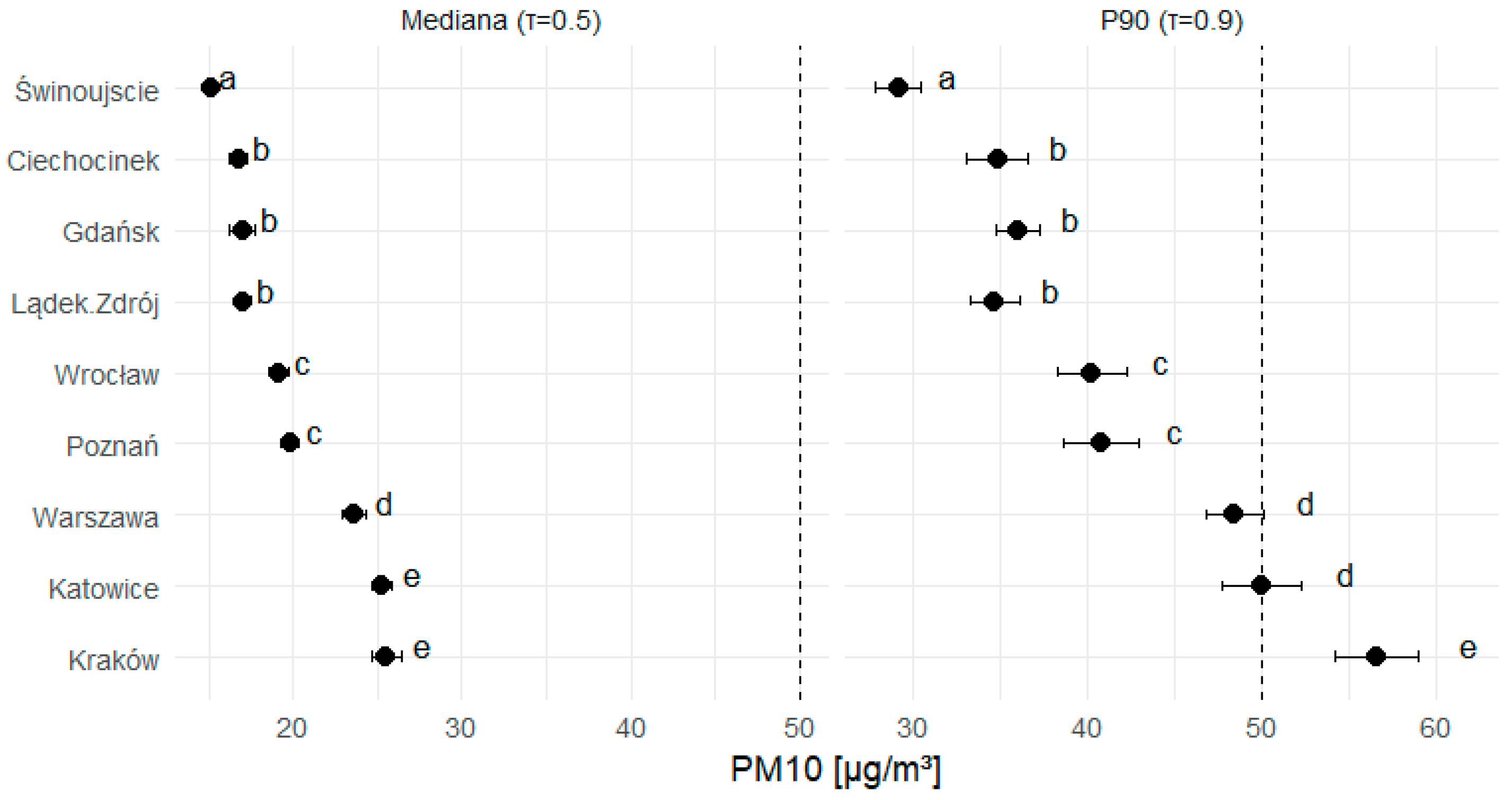
Overall, the results of quantile regression indicate that differences between locations are much greater during episodes of high pollution (90th percentile) than on typical days (median)—Figure 10. This means that Kraków, Katowice, and Warsaw are particularly exposed to extreme smog episodes, while Świnoujście and Ciechocinek remain relatively less affected. For reliable confidence intervals and contrast tests, a bootstrap covariance matrix of estimates was applied. Marginal means (on the µg/m³ scale) and their 95% confidence intervals (CI) were calculated, and multiple comparisons were adjusted using the Benjamini–Hochberg method. The results are presented in Figure 10 as a plot with point estimates and CLD letters indicating homogeneous groups (locations marked with the same letter do not differ significantly). The median and P90 from quantile regression are shown in Figure 11. Letters above the points indicate homogeneous groups.

The quantile regression analysis for the median (τ = 0.5) revealed significant differences in PM10 levels between locations (

Table 3. Results of quantile regression for the median (τ = 0.5) of PM10 concentrations [µg/m³] in the analyzed locations.

Location	Level	LCL	UCL	p_BH_tau0.5	p_Label
Ciechocinek	16.73	16.208	17.251	NA	ref
Gdańsk	17.00	16.417	17.582	4.98$\times 10^{-1}$	0.498
Katowice	25.20	24.531	25.869	1.42$\times 10^{-83}$	<0.001
Kraków	25.50	24.714	26.285	4.82$\times 10^{-73}$	<0.001
Lądek.Zdrój	17.07	16.604	17.535	3.88$\times 10^{-1}$	0.389
Poznań	19.81	19.254	20.365	4.88$\times 10^{-15}$	0.001
Świnoujscie	15.10	14.724	15.475	8.79$\times 10^{-7}$	<0.001

).

With reference to Ciechocinek (16.73 µg/m³; 95% CI: 16.21–17.25), the highest median values were observed in industrial agglomerations, namely Kraków (25.50 µg/m³; 95% CI: 24.71–26.29; p(BH) < 0.001 compared to the reference), Katowice (25.20 µg/m³; 95% CI: 24.53–25.87; p(BH) < 0.001), and Warsaw (23.59 µg/m³; 95% CI: 22.98–24.20; p(BH) < 0.001). Significantly lower medians were recorded in Świnoujście (15.10 µg/m³; 95% CI: 14.72–15.48; p(BH) < 0.001), suggesting a more favorable air quality background in the coastal location. For Gdańsk (17.00 µg/m³; p(BH) = 0.498) and Lądek-Zdrój (17.07 µg/m³; p(BH) = 0.389), no significant differences were found compared to the reference location. Poznań (19.81 µg/m³; p(BH) < 0.001) and Wrocław (19.10 µg/m³; p(BH) < 0.001) occupied an intermediate position, with moderately higher median PM10 values.

In turn, the quantile regression analysis for the 90th percentile (τ = 0.9) revealed much stronger differences between locations than in the case of the median, indicating that the variability of PM10 concentrations increases during high-pollution episodes (

Table 4. Results of quantile regression for the 90th percentile (τ = 0.9) of PM10 concentrations [µg/m³] in the analyzed locations.

Location	Level	LCL	UCL	p_BH_tau0.9	p_Label
Ciechocinek	34.86	33.251	36.468	NA	ref
Gdańsk	36.00	34.528	37.471	3.48$\times {10}^{-1}$	0.349
Katowice	50.00	47.744	52.255	2.86$\times {10}^{-26}$	<0.001
Kraków	56.61	53.844	59.375	2.017$\times {10}^{-39}$	<0.001
Lądek.Zdrój	34.71	33.356	36.063	8.88${\times 10}^{-1}$	0.889
Poznań	40.81	38.828	42.791	7.85$\times {10}^{-6}$	<0.001
Świnoujscie	29.21	28.082	30.337	3.51${ \times 10}^{-8}$	<0.001

).

With reference to Ciechocinek (34.86 µg/m³; 95% CI: 33.25–36.47), the highest P90 values were observed in Kraków (56.61 µg/m³; 95% CI: 53.84–59.38; p(BH) < 0.001) and Katowice (50.00 µg/m³; 95% CI: 47.74–52.26; p(BH) < 0.001), indicating a clearly higher frequency of smog episodes in these locations. High P90 values were also recorded in Warsaw (48.44 µg/m³; p(BH) < 0.001), while Poznań (40.81 µg/m³; p(BH) < 0.001) and Wrocław (40.30 µg/m³; p(BH) < 0.001) occupied an intermediate position. In contrast, Świnoujście (29.21 µg/m³; 95% CI: 28.08–30.34; p(BH) < 0.001) showed a significantly lower P90 compared to the reference, suggesting a lower frequency of high PM₁₀ concentrations in this location. Gdańsk (36.00 µg/m³; p(BH) = 0.349) and Lądek-Zdrój (34.71 µg/m³; p(BH) = 0.889) did not differ significantly from the reference location, indicating a moderate level of pollution episodes. Overall, the P90 results clearly emphasize that differences between locations are most pronounced in the upper quantiles of the PM₁₀ concentration distribution, confirming the crucial role of smog episodes in shaping air quality variability in Poland.

The results of the quantile regression revealed a clear asymmetry in the spatial variability of PM₁₀ concentrations. While the differences between locations in the central value of the distribution (median, τ = 0.5) were moderate, much greater disparities appeared in the upper quantile (τ = 0.9), which reflects smog episodes. This indicates that environmental inequalities between locations are primarily revealed under high-pollution conditions rather than on typical days. For instance, the 90th percentile reached 56.6 µg/m³ in Kraków and 50.0 µg/m³ in Katowice, whereas in Świnoujście it was only 29.2 µg/m³ (

Table 5. Mean values and 90th percentile.

Location	Mean_pm10	p90_pm10
Kraków	31.157	56.605
Katowice	30.172	49.990
Warszawa	27.903	48.436
Poznań	23.881	40.801
Wrocław	23.056	40.300
Gdańsk	20.442	35.990
Lądek.Zdrój	20.051	34.709

). This represents a difference of +27.4 µg/m³ and +20.8 µg/m³, respectively, compared to areas with the lowest emission levels. Such analysis makes it possible to capture phenomena that remain invisible in models based on means or medians.

The results indicate that episodic high PM₁₀ concentrations, rather than annual mean levels, are the main source of air quality variability in Poland. The highest values were observed in southern agglomerations, where the accumulation of pollutants is influenced by both emission factors (solid fuel heating, dense urban development) and meteorological conditions such as air stagnation and winter temperature inversions. This suggests that assessing air quality solely based on mean values may lead to misleading conclusions, and that mitigation measures should focus on reducing episodic pollution events.

4. Discussion

Table 6. Percentage rate of change of PM₁₀ in 2019–2024.

Location	2019	2024	cagr_pct	Change_pct_Total
Warszawa	37.742	22.099	−10.151	−41.447
Katowice	41.135	26.335	−8.532	−35.978
Świnoujscie	21.751	14.987	−7.177	−31.093
Poznań	27.749	22.425	−4.171	−19.186
Kraków	35.255	29.015	−3.821	−17.698
Lądek.Zdrój	24.275	20.539	−3.286	−15.389
Ciechocinek	21.187	18.087	−3.113	−14.629
Gdańsk	20.219	18.623	−1.631	−7.891
Wrocław	24.073	22.781	−1.098	−5.3721

presents the percentage rate of change in PM₁₀ from 2019 to 2024 for key locations.

cagr_pct—represents the Compound Annual Growth Rate (CAGR), indicating the average annual percentage change in PM₁₀ concentrations between 2019 and 2024.

Change_pct_Total—denotes the total percentage change over the period 2019–2024, showing the overall decrease (or increase) in PM₁₀ concentrations from 2019 to 2024.

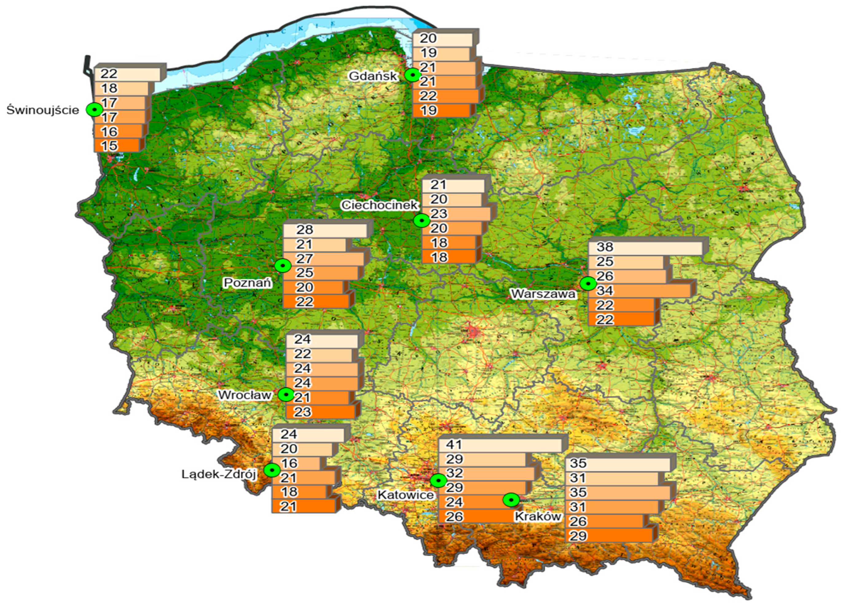
To visualize temporal and spatial trends, GIS mapping of average annual data was also performed (Figure 12). The data is arranged from the darkest color, i.e., the oldest (2019), to the lightest, i.e., the newest (2024).

The observed downward trends in PM10 concentrations are likely the result of the combined influence of several social, technological, and environmental factors [37]. First, during the analyzed period, Poland implemented an increasingly intensive anti-smog policy, including regional anti-smog resolutions in the Małopolskie and Silesian voivodeships (banning the use of non-certified boilers) and the “Clean Air” program, which promotes the replacement of heating sources and the thermal modernization of residential buildings. Second, cities undertook measures to reduce traffic-related emissions, such as the introduction of low-emission transport zones, modernization of bus fleets, and the expansion of electric and gas infrastructure. Third, the observed changes may also have been influenced by meteorological factors, particularly milder winters during some seasons of the analyzed period and variations in air circulation patterns that may reduce the frequency of strong temperature inversions.

However, it should be emphasized that in southern Poland, the process of emission reduction is slower due to the high share of individual coal-based heating and specific topographic conditions that favor the accumulation of pollutants. The findings of this study highlight the need for further research in this area, particularly in regions with persistently high low-stack emissions and during periods of increased demand for thermal energy [38].

The analysis of data from 2019 to 2024 revealed significant differences in PM₁₀ concentration levels between the studied locations. Both classical tests (Welch ANOVA, permutation test) and statistical models (LMM, GAM, quantile regression) consistently indicated that the highest PM₁₀ concentrations occurred in large agglomerations—Kraków, Katowice, and Warsaw—while the lowest were observed in Świnoujście. Poznań and Wrocław occupied intermediate positions, whereas Ciechocinek, Gdańsk, and Lądek-Zdrój did not differ significantly from one another or from the reference values.

The mixed model (LMM) showed that, after controlling for common daily fluctuations, location-based differences remained stable, with the largest contrasts observed between agglomerations and Świnoujście. The GAM model additionally confirmed strong seasonality (winter maximum, summer minimum) and diverse temporal trends—ranging from simple, nearly linear trends in Kraków and Ciechocinek to more complex patterns in Warsaw, Gdańsk, and Lądek-Zdrój. After accounting for seasonality, some contrasts (e.g., Katowice–Kraków, Poznań–Wrocław) lost significance, indicating that these differences stemmed mainly from varying seasonal trend structures. Quantile regression, in turn, revealed that differences between locations were particularly pronounced in the upper tail of the distribution (90th percentile), i.e., during smog episodes—when values in Kraków exceeded those in the reference Ciechocinek by as much as 22 µg/m³.

Quantile analysis has significant practical importance, as it reflects the health risks associated with sudden and intense smog episodes. The results of this study confirm that population exposure is not determined by average PM₁₀ concentrations but rather by extreme values that occur seasonally, particularly during the heating period. At the same time, the highest risk of exceeding permissible PM₁₀ limits concerns the Silesian and Kraków agglomerations, which is consistent with previous observations and reports by the EEA and WHO. Consequently, air quality policy should take into account rapid-response mechanisms to smog episodes (e.g., temporary emission restrictions, low-emission zones, public alerts) rather than focusing solely on programs aimed at reducing annual mean PM₁₀ levels.

The conducted study also shows that quantile regression is a valuable tool in environmental analysis, as it allows for capturing variations in emission and pollutant transport conditions that are overlooked by classical linear models.

Thus, large agglomerations (Kraków, Katowice, Warsaw) are characterized by the highest and most problematic PM₁₀ levels, both in terms of averages and during smog episodes. Świnoujście and spa towns (Ciechocinek, Lądek-Zdrój) exhibit significantly lower values, confirming their more favorable environmental conditions and justifying their spa status. Seasonality undoubtedly plays a key role—with the highest values recorded in winter and the lowest in summer—reflecting the impact of communal heating and meteorological conditions.

The observed spatial variability of air quality has clear emission-related and environmental determinants. The highest PM₁₀ concentrations were recorded in Kraków, Katowice, and Warsaw, which is consistent with the influence of two main groups of sources: traffic-related emissions associated with intensive road transport and so-called low-stack emissions originating from individual solid fuel heating systems. In the Upper Silesia and Małopolska regions, an additional contributing factor is dense urban development located in areas unfavorable for air ventilation, as well as temperature inversion phenomena that lead to the accumulation of pollutants in the near-surface layer of the atmosphere [39]. Conversely, lower concentrations in locations such as Lądek-Zdrój or Świnoujście result from lower traffic intensity and more favorable dispersion conditions, particularly in coastal zones where higher wind speeds promote the dilution of atmospheric aerosols.

The downward trends observed in 2019–2024 were significantly influenced by regulatory and investment measures implemented at both national and regional levels. In the Małopolskie and Silesian voivodeships, anti-smog resolutions were introduced, mandating the replacement of inefficient furnaces and imposing restrictions on the use of solid fuels. At the same time, support programs such as “Clean Air” contributed to an increase in the number of buildings undergoing thermal modernization and being equipped with less polluting heating systems [40].

It should also be emphasized that the analyzed phenomena exhibit strong seasonality, resulting from increased demand for thermal energy during the winter period and meteorological conditions that limit pollutant dispersion (high pressure, lack of convection, weak wind). The GAMs applied in this study confirmed this effect, indicating a recurring winter peak in concentrations across all analyzed locations.

The study faced certain limitations related to meteorological variables, which resulted from the availability of measurement data. Meteorological variables (e.g., temperature, wind speed, relative humidity, precipitation) were not included due to the lack of consistent, co-located daily time series for all analyzed monitoring points in the years 2019–2024. A potential part of their influence was indirectly captured in the LMM through the random day effect, which models shared episodes (often weather-driven), and in the GAM through a cyclic spline of the day of the year as a proxy for meteorological seasonality. Nevertheless, the absence of explicit meteorological predictors limits the causal interpretation of differences between locations; therefore, in future research, the authors plan to integrate meteorological data and assess the robustness of the results using a multimodel approach extended to include weather-related variables.

The applied methodological approach, although based on well-established statistical techniques, is characterized by an innovative, application-oriented integration of methods with complementary properties. This combination made it possible not only to distinguish pollution levels between locations but also to separate the effects of seasonality and long-term trends from episodic phenomena. Particularly important was the use of quantile regression as a tool for analyzing extreme smog episodes, which are crucial from a public health perspective yet often insufficiently addressed in the national literature. Moreover, incorporating a random day effect in the LMM model helped to avoid the underestimation of standard errors resulting from temporal autocorrelation, which can be considered a methodological strength of the study. In addition, the consistent application of the FDR control procedure increased the reliability of comparisons between locations by reducing the risk of errors arising from multiple testing. Such an integrated combination of environmental data modeling techniques has not been previously reported in studies on air quality in Poland, highlighting the applied contribution of this work and its potential significance for future research and analyses conducted by air quality monitoring institutions.

The added value of this study lies in the application of consistent and methodologically complementary analytical techniques to assess complex environmental phenomena in Poland within a spatio-temporal framework. The originality of the work is application-oriented and is reflected in the following aspects:

• A comprehensive comparison of three types of areas—large agglomerations, medium-sized cities, and spa towns—in the context of emission variability and the effects of environmental policy;
• Inclusion in the analysis not only of mean concentration levels but also of smog episodes, which made it possible to identify locations particularly exposed to exceedances of daily PM₁₀ limits;
• The use of linear mixed models to eliminate temporal covariation and to separate local effects from nationwide pollution episodes;
• The analysis of long-term trends and seasonality using GAMs, which enabled the identification of structural differences in the temporal evolution of air quality;
• The application of quantile regression, through which stronger inter-location differences were demonstrated in the upper quantiles of the distribution (τ = 0.9), which is highly relevant for health risk assessment.

Furthermore, the obtained results contribute to the existing body of knowledge in the field of air quality monitoring in Poland and Central and Eastern Europe, highlighting the persistence of regional environmental disparities despite the overall downward trend. The study may serve as a basis for the development of territorially differentiated anti-smog policies, particularly in the context of the planned updates to the National Air Protection Program and the initiatives implemented under the European Green Deal.

5. Conclusions

The aim of this study was to address the research questions concerning the development of long-term air quality trends in Poland based on PM₁₀ concentrations, as well as to identify differences between urban agglomerations, smaller towns, and spa resorts. The analysis revealed a clear downward trend in PM₁₀ levels over the study period, consistent with the EU’s objectives under the European Green Deal and the long-term goal of environmental neutrality by 2050. At the same time, significant spatial disparities were observed—the largest urban centers remain the most burdened by pollution, whereas spa towns maintain relatively stable air quality.

From the perspective of environmental policy, these findings are of critical importance. They show that the overall improvement in air quality does not guarantee uniform outcomes across the country. To realistically meet EU targets, political and economic actions must be directed towards the most exposed areas—particularly large agglomerations, where the combined effects of transport, industry, and emissions from the residential and communal sector accumulate. This implies the need to introduce more stringent local air quality standards, invest in zero-emission heating systems, accelerate the energy transition based on renewable sources, and expand sustainable urban transport.

The differences between large urban agglomerations and spa towns are as much as 22 µg/m³ during the period of the highest PM₁₀ concentrations. Referring to Table 6, the city with the largest percentage decrease, which is −41%, is Warsaw, and Katowice −35%. The cities with the smallest percentage decrease are Wrocław (−7%) and Gdańsk (−5%). These differences result, according to the Central Statistical Office, from the greater financial contribution received to the development of eco-friendly policies in the cities of Warsaw and Katowice [40]. As demonstrated by the presented analysis, political actions for climate change are actually reflected in practice.

The analysis of seasonal fluctuations in PM₁₀ concentrations, especially during winter, clearly indicates that without decisive political interventions in the area of individual heating and improvements in building energy efficiency, achieving the 2050 targets remains highly problematic. The results demonstrate that existing policy mechanisms must be supplemented with solutions tailored to regions with the highest pollution levels, as well as tools to monitor the effectiveness of their implementation.

In summary, the study confirms that Poland is on the right track in reducing air pollution. However, achieving the ambitious EU goals requires a much more differentiated political approach, adapted to local conditions. Without this, the risk of delays in fulfilling EU commitments remains substantial. The authors plan to extend the research to other EU member states in order to assess whether similar challenges and disparities occur on a European scale, which would enable the development of joint and more effective environmental policy strategies.