Hybrid A-Star Path Planning Method Based on Directional Guidance and Segment-Based Heuristic Weighting

Abstract

To improve the planning efficiency of the Hybrid A-Star algorithm in facility-based agriculture environments, we propose a novel method that integrates directional guidance and segment-based heuristic weighting. Jump point search (JPS) is first employed to generate a reference path, from which key jump points and their heading angles are extracted to guide node expansion. The path is then segmented into straight and turning segments, each assigned dynamic heuristic weights to form a segment-wise heuristic sequence. Simulation results show that, while maintaining comparable path lengths, the proposed method significantly improves computational efficiency, reduces node expansion, and enhances overall path smoothness. These results highlight the proposed method’s effectiveness for path planning in autonomous mobile platforms operating within agricultural facilities.

1. Introduction

Under the dual pressures of continuous global population growth and tight arable land resources, the smart agricultural system, with the core goals of precision, efficiency, and sustainability, is developing rapidly. Aiming to increase agricultural output and resource utilization efficiency, reduce labor intensity, and ensure food safety, smart agriculture uses technologies such as the Internet of Things (IoT), big data, artificial intelligence, and robotics to monitor and make decisions on the environment, soil, crop growth conditions, and production processes in real time [1,2,3]. In facility-based agriculture such as greenhouse farms, key indicators such as temperature, humidity, light and water, and fertilizer can be precisely monitored and managed. The automation and intelligence of agricultural equipment is another important aspect to ensure the efficient and stable production process.

Against this backdrop, the automatic navigation technology for agricultural machinery is a key element of smart agriculture, with path planning constituting the core of such systems [4,5]. In facility-based environments such as greenhouses, the working areas are mostly characterized by multiple rows of symmetry, narrow and long corridors, and dense obstacles. When performing tasks, intelligent transportation vehicles need to pass through complex U-shaped areas, and this poses significant challenges to the robustness and safety of the path planning. To ensure the crops are not damaged and to enhance the delivery efficiency, the planned path not only needs to comply with the kinematic constraints of the vehicle but also needs to generate a feasible trajectory with low oscillation and high smoothness and maintain an adequate safety distance from the corridor walls and obstacles.

Conventional path planning algorithms primarily encompass graph search-based methods (e.g., A-star and Dijkstra), sampling-based approaches (e.g., RRT), optimization-based techniques (e.g., gradient descent), and curve interpolation methods (e.g., Dubins and Bézier curves) [6]. Among these, the A-star algorithm is commonly used for global path planning in static maps due to its stability and heuristic characteristics [7,8]. A-star algorithm uses a heuristic function to search for the shortest path on a grid map. However, in situations with dense obstacles, it is prone to generating a large number of redundant nodes and resulting in decreased computational efficiency [9]. In a real agricultural environment, the A-star algorithm faces challenges such as excessive node expansion, abrupt curvature changes, and inability to accommodate dynamic constraints [10,11].

To address these issues, the Hybrid A-star algorithm was developed. This method combines the heuristic search framework of A-star with the trajectory generation mechanism in continuous space. It enhances the feasibility and smoothness of the path by integrating kinematically feasible extension strategies (such as Reeds-Shepp or Dubins paths) [12,13]. The Hybrid A-star algorithm has demonstrated excellent performance in automatic parking [14,15,16], complex structural environments, and intelligent agricultural scenarios [17,18,19].

To further enhance the path planning performance of the Hybrid A-star algorithm in complex constraint environments, researchers have proposed various improvement strategies. From the standpoint of path continuity, some researchers apply Bézier curves or cubic splines to smooth the discrete paths generated by the Hybrid A-star algorithm, which enhance the stability of path tracking control [20]. Some studies have incorporated G2 continuity constraints during the path generation stage to ensure the smoothness of curvature changes, thereby improving path quality and compatibility with vehicle control systems [21]. To address the challenges of excessive node expansions in the Hybrid A-star algorithm when dealing with high-resolution maps, Cui et al. [22] proposed an improved method based on geometric curves and direction guidance. During the planning stage, multiple controllable arcs are implemented, and the path expansion direction is dynamically guided by the local geometric structure, effectively reducing the expansion of invalid nodes and improving the search efficiency. To further reduce the search space, some studies have incorporated the Jump Point Search (JPS) algorithm into the initial guidance stage of the ant colony optimization. As reported in the literature [23], initializing pheromone distribution with jump points expedites early iterations by directing the algorithm toward more promising solution regions. The above studies all demonstrate that the Hybrid A-star algorithm has excellent scalability and integration capabilities and is suitable for path planning tasks in facility agriculture that involve multiple types of obstacles and highly coupled kinematic constraints.

In recent years, research on path planning for facility-based agricultural such as greenhouses and orchards has exhibited significant trends of integration, multi-level structure, and high real-time performance. In orchard operation, in order to meet the actual requirements of the grass-cutting robot for operation in the dense planting rows, Li et al. [24] proposed a path generation strategy based on safety corridors and secondary planning. Their approach divides the environment into high-security zones and drivable areas and then performs trajectory optimization. It effectively avoids obstacles while maintaining high controllability. For articulated tractor path optimization, some scholars have utilized a multi-objective function that integrates genetic algorithms with a multi-segment structure encoding method to comprehensively optimize the path length, the number of turns, and the alignment accuracy. It demonstrates that multi-dimensional performance indicators are gradually gaining attention in agricultural path planning [25]. Overall, agricultural path planning is progressing towards structural adaptation and model integration, emphasizing the deployability and stability of algorithms in actual operation systems.

However, in large-scale greenhouse or multi-narrow corridor environments, the conventional Hybrid A-star algorithm often exhibits insufficiencies in node expansion owing to unnecessary exploration into dead zones. The adopted fixed heuristic poses challenges in balancing search efficiency with path quality. To overcome these limitations, this study proposes a novel Hybrid A-star algorithm path planning method based on directional guidance and segmented heuristic weighting, which takes into account both search efficiency and path feasibility. The proposed approach introduces two principal enhancements: directional node expansion and adaptive heuristic weighting. First, the JPS algorithm is employed to extract key jump points from the planned path and utilize them as the direction guiding points for the Hybrid A-star algorithm. The guiding nodes expand successively in the direction of the key jump points to avoid the ineffective node expansion. Secondly, by calculating the difference in reference heading angles between adjacent key jump points and combining with axis alignment detection, determine whether the current path segment is a straight segment or a turning segment. Higher heuristic weights are allocated to straight segments to accelerate the search process along linear corridors, whereas lower weights are retained for turning segments to preserve trajectory smoothness and planning quality.

2. Proposed Path Planning Framework and Methodology

2.1. Overview of the Proposed Path Planning Framework

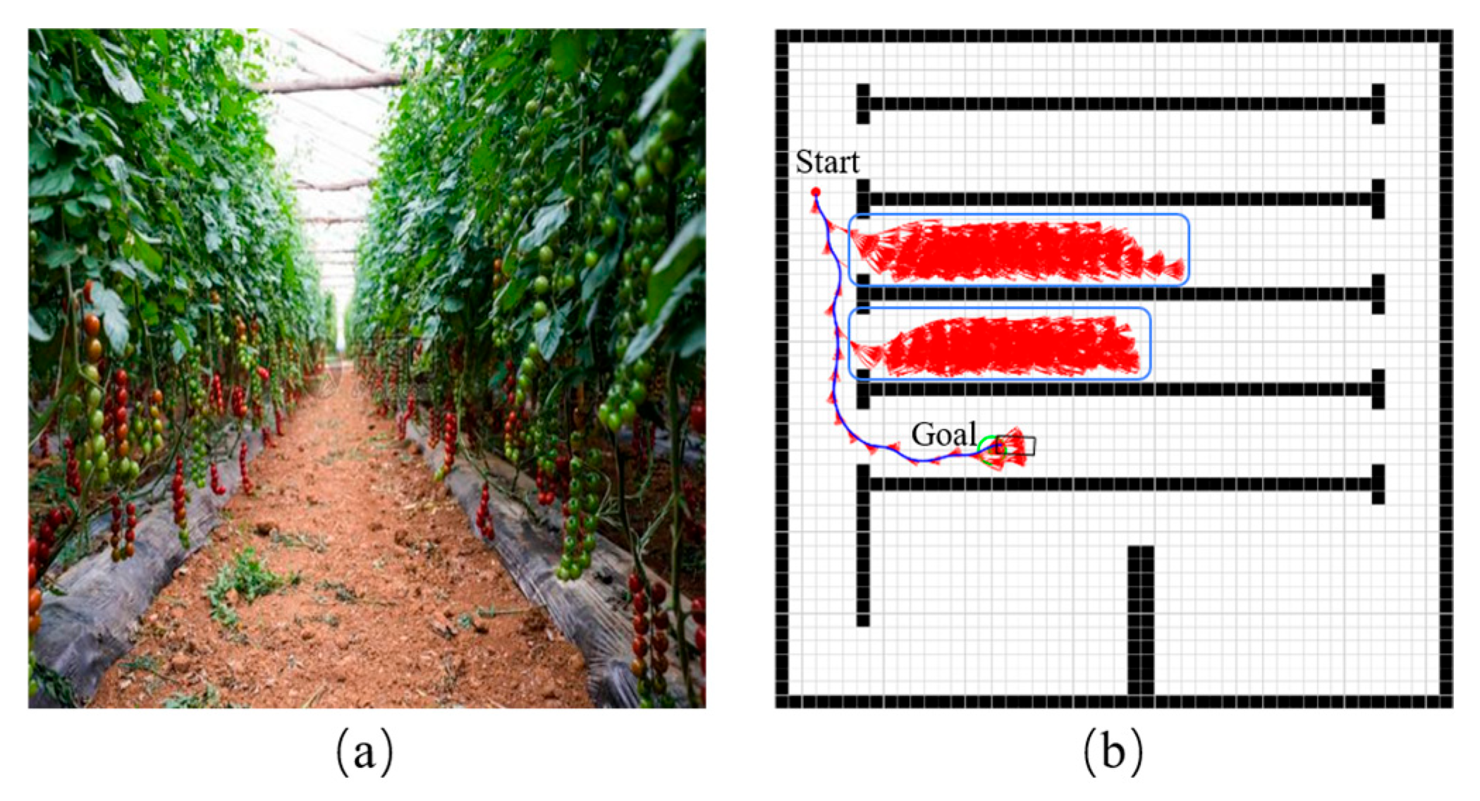
In structured agriculture environments such as greenhouses, U-shaped obstacles are frequently encountered. When applying the Hybrid A-star algorithm for path planning in these settings, the search process often extends into dead zones, resulting in a large number of invalid node expansions and decreased computational efficiency. As shown in Figure 1a, a typical tomato greenhouse is depicted. For path planning purposes, the structural layout of the greenhouse is abstracted into a 2D grid map. Figure 1b shows the corresponding path generated by the Hybrid A-star algorithm. In the grid representation, black cells indicate obstacle regions, white cells represent navigable workspace, and the blue box underscores an area where the algorithm expands into a dead zone, leading to inefficient and unnecessary node exploration.

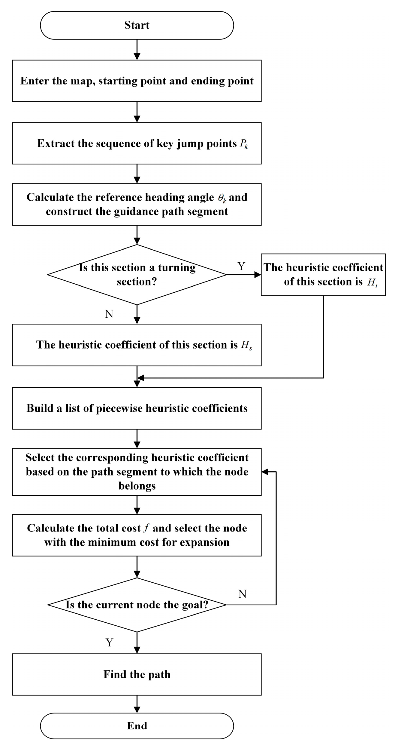
A preliminary path is quickly generated using the JPS algorithm between the start and goal positions, from which a sequence of key jump points is extracted. These jump points act as directional references for the subsequent Hybrid A-star planning process, effectively reducing unnecessary exploration into dead zones. For each jump point, a reference heading angle is calculated based on the coordinates of two adjacent jump points. By analyzing heading angle differences and axis alignment between successive segments, the path is classified into either turning or straight segments. Each segment is then assigned a dynamic heuristic coefficient, resulting in a segment-wise heuristic coefficient list. This allows accelerated node expansion in straight-line regions and enhanced path smoothness in turning regions. When the expanding node enters a predefined tolerance region around the next jump point, the algorithm switches to the corresponding heuristic coefficient for that segment. The total cost function integrates the travel cost, steering continuity penalty, and directional deviation penalty, thereby promoting efficient forward exploration while constraining node expansion in non-optimal directions. The overall algorithm workflow is shown in Figure 2.

2.2. Vehicle Kinematic Model and Node Expansion Strategy

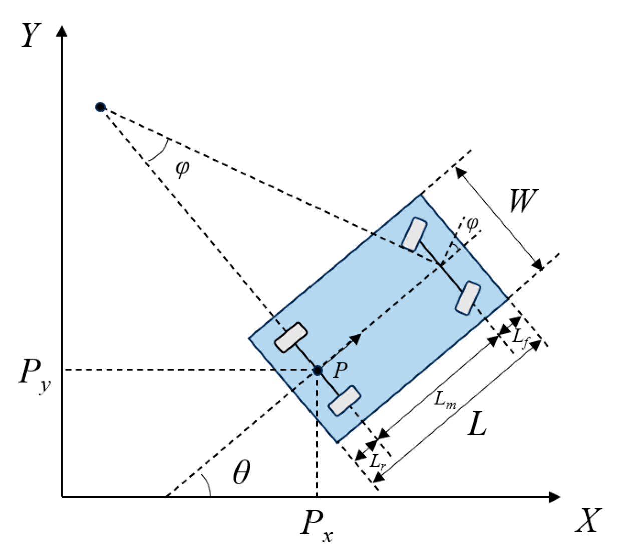
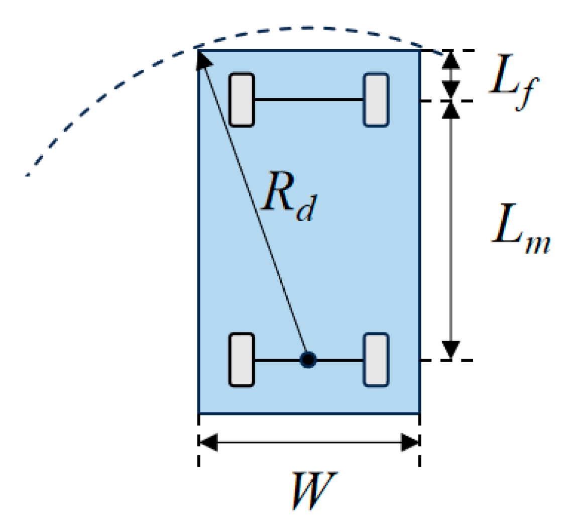
The improved Hybrid A-star algorithm proposed in this study is formulated based on an Ackermann-steering vehicle model. The kinematic structure of the Ackermann model is presented in Figure 3. In the diagram, $(P_x,P_y)$ represent the coordinates of the rear axle center, $\theta$ denotes the vehicle’s orientation (heading angle), and $\phi$ represents the front-wheel steering angle. In addition to these motion parameters, the figure also presents key geometric parameters of the vehicle, including $L$ (vehicle length), $L_f$ (front overhang), $L_m$ (wheelbase), $L_r$ (rear overhang), and $W$ (vehicle width). Based on the Ackermann kinematic constraints and the vehicle’s geometric configuration, the minimum turning radius $R_{min}$ can be calculated as:

$$R_{min}={\displaystyle \frac{L_m}{tan{\phi }_{max}}}$$

(1)

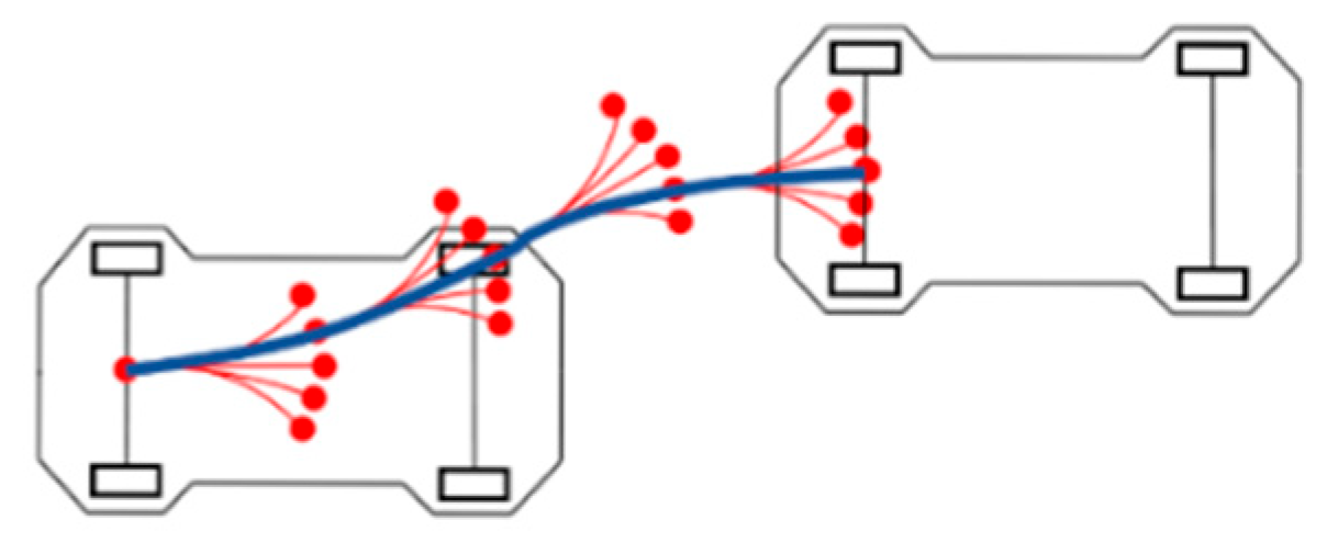
The Hybrid A-star algorithm enhances the conventional A-star algorithm by incorporating the vehicle’s kinematic constraints, thereby allowing the generation of paths that are physically feasible and trackable by real vehicles. Unlike the A-star algorithm, which expands nodes strictly based on adjacent grid centers, the Hybrid A-star algorithm utilizes a set of discrete motion primitives defined by step length, turning radius, and front wheel steering angles, as shown in Figure 4. The red line segments correspond to expansion trajectories, red dots mark the expanded nodes, and the blue solid line shows the generated path. This approach allows successor nodes to occupy arbitrary positions within the grid, rather than being confined to grid cell centers as in the standard A-star algorithm. As a result, the Hybrid A-star algorithm more accurately models continuous motion and supports the planning of kinematically feasible trajectories.

The state of the vehicle is represented by the position and heading angle of the rear-axle center, denoted as $s=(P_x,P_y,q)$. Assuming each control input consists of a linear displacement $D$ and a front-wheel steering angle $\phi$, the relationship between the current node and its successor node can be described using the following kinematic equations:

$$\left\{\begin{array}{c}{P}_{x(i+1)}=P_{x(i)}+D\cos ({\theta }_i)\\ P_{y(i+1)}=P_{y(i)}+D\sin ({\theta }_i)\\ {\theta }_{i+1}={\theta }_i+{\displaystyle \frac{D}{L}}\tan \phi \end{array}\right.$$

(2)

2.3. Jump Point-Based Global Guidance Mechanism

The JPS algorithm is an optimized variant of the conventional A-star algorithm. In the standard A-star approach, each node expansion involves evaluating potential movements in all eight directions around the current node, making the computation process relatively complex and time-consuming. JPS enhances efficiency by eliminating unnecessary intermediate nodes and retaining only a set of representative key nodes, referred to as jump points, to guide the search. These jump points allow the algorithm to reduce redundancy and accelerate the overall path planning process.

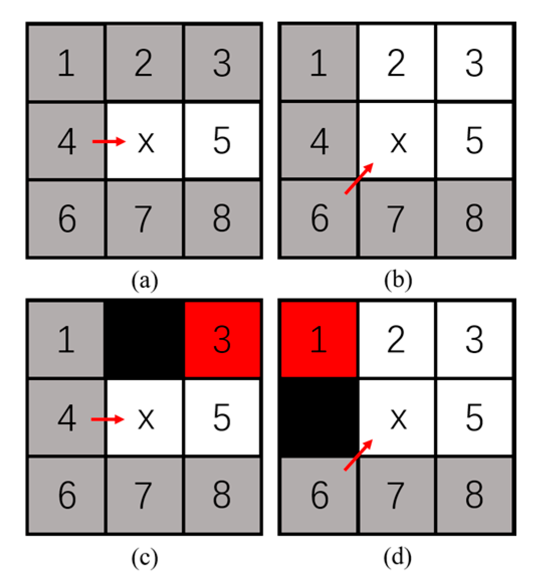
Based on the distribution of obstacles in the map, the neighboring nodes around a given node can be categorized into two types: natural neighbors and forced neighbors. For example, in the absence of surrounding obstacles, consider a scenario where the parent node expands horizontally from node 4 to node $x$. If a neighboring node $n$ satisfies the condition that the path passing through $x$ is shorter than any alternative path that avoids $x$, then $n$ is identified as a natural neighbor. This relationship is illustrated by the gray cells in Figure 5a.

When the expansion direction is either horizontal or vertical, the criteria for identifying natural neighbors can be formally defined as follows:

$$L(P(x),\cdots ,n)\ge L(P(x),x,n)$$

(3)

where $L(·)$ represents path length; $<P(x),\dots ,n>$ denotes a path from $P(x)$ to $n$ that does not pass through $x$; $<P(x),x,n>$ denotes the path $P(x)\to x\to n$; $P(x)$ is the parent node of $x$. When expanding diagonally from parent node 6 to node $x$, a neighboring node $n$ is considered a natural neighbor if the path that passes through node $x$ is longer than the alternative path that bypasses $x$, as illustrated in Figure 5b. This condition typically occurs during diagonal expansions under specific geometric constraints.

In an obstacle-free environment, when the expansion direction is diagonal, the criteria for identifying natural neighbors can be defined as follows:

$$L(P(x),\cdots ,n)>L(P(x),x,n)$$

(4)

When obstacles are present around the current node, a neighboring node $n$ is identified as a forced neighbor if the cost of the path passing through node $x$ from the parent node is lower than the cost of bypassing $x$ to reach $n$. In other words, the presence of an obstacle forces the path to include node $x$ to maintain optimality. Such nodes are highlighted in red in Figure 5c,d, which illustrate typical scenarios where forced neighbors arise owing to the presence of adjacent obstacles.

A neighboring node $n$ is considered a forced neighbor if it satisfies both of the following conditions:

(1)

Node $n$ is not a natural neighbor;

(2)

The path passing through node $x$ from the parent node has a lower total cost than any alternative path reaching $n$ that avoids $x$.

A node $x$ is identified as a jump point if it satisfies at least one of the following conditions:

(1)

Node $x$ is the start or end point;

(2)

Node $x$ has at least one forced neighbor;

(3)

When expanding diagonally, both the horizontal and vertical neighbors of $x$ satisfy either condition 1 or 2;

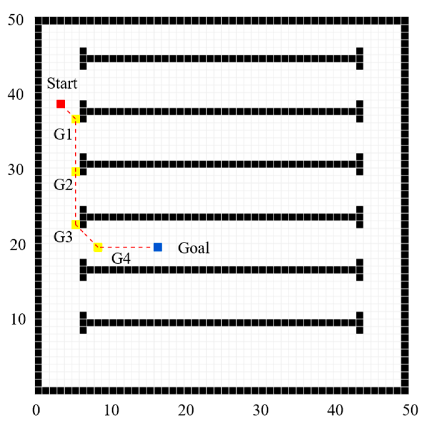
The path is initially planned on the grid map using the JPS algorithm. Based on the jump point selection criteria, key jump points are extracted from the resulting path and serve as directional guidance references for the Hybrid A-star algorithm. The selection of key jump points is illustrated in Figure 6.

2.4. Design of Tolerance Region Around Key Jump Points

To ensure collision-free path planning and enable node expansion into regions guided by key jump points, a tolerance region is defined around each jump point, as illustrated in Figure 7. This tolerance area also enhances the continuity between different path segments that are assigned different heuristic weights.

The tolerance region is defined as a circular area centered at each jump point, with its radius determined based on the vehicle’s geometric dimensions. Let $R_d$ represent the diagonal distance from the rear-axle center to the frontmost point of the vehicle. Given $L_f$ (front overhang), $L_m$ (wheelbase), and $W$ (vehicle width), the radius $R_d$ of the positional tolerance region is expressed as:

$$R_d=\sqrt{{(L_m+L_f)}^2+{({\displaystyle \frac{W}{2}})}^2}$$

(5)

This tolerance ensures that any node entering the vicinity of a jump point can be considered to have successfully reached it, thereby facilitating smooth heuristic transitions and stable trajectory continuity across path segments.

2.5. Segment-Based Heuristic Weighting Strategy

In the traditional Hybrid A-star algorithm, the heuristic weight $H_{cost}$ is typically held constant throughout the planning process. However, maintaining a constant heuristic coefficient makes it challenging to strike an optimal balance between search efficiency in straight-line segments and path smoothness in turning segments. To overcome this limitation, a segment-based heuristic weighting mechanism is proposed. By calculating the heading angle difference between two adjacent key jump points and determining their axis alignment, each path segment is categorized as either a straight or a turning segment. Distinct heuristic weights are then assigned based on this classification: higher weights are used in straight segments to accelerate the search, whereas lower weights are used in turning segments to preserve path quality.

Because the key jump points extracted from the JPS algorithm lack heading information, a reference heading angle ${\theta }_k$ is computed for each key jump point (excluding the start and goal points), based on the coordinates of its adjacent jump points. The reference heading angle ${\theta }_k$ for the $k$ jump point is calculated as:

$${\theta }_k=atan2(y_{k+1}-y_k,x_{k+1}-x_k)$$

(6)

where $P_{k+1}(x_{k+1},y_{k+1})$ and $P_k(x_k,y_k)$ are the coordinates of two adjacent jump points, respectively.

To classify path segments and assign appropriate heuristic weights, both the heading angle difference and axial alignment are evaluated for all pairs of adjacent key jump points, including the start and goal points. A path segment between two consecutive jump points $P_{k+1}$ and $P_k$ is classified as a turning segment if either of the following conditions is met:

(1)

The absolute difference between their reference heading angles exceeds a predefined threshold ${\theta }_s$;

(2)

The two points are not aligned along the same axis (i.e., they are not directionally collinear).

Otherwise, the segment is classified as a straight segment. The heuristic weight $H_i$ for each segment is assigned accordingly:

$$H_i=\left\{\begin{array}{l}{H}_t,\mathrm{\Delta }\theta >{\theta }_s\wedge \left(x_i\ne x_{i+1}\wedge y_i\ne y_{i+1}\right)\\ H_s=min\left\{\left(1+{\displaystyle \frac{{\theta }_s}{\mathrm{\Delta }\theta }}\right)H_t,H_{\mathit{\text{s-max}}}\right\},\mathrm{\Delta }\theta \le {\theta }_s\end{array}\right.$$

(7)

$$\mathrm{\Delta }\theta =\left|{\theta }_{k+1}-{\theta }_k\right|$$

(8)

These parameters were empirically tuned through multiple preliminary simulations to balance path smoothness and computational efficiency, and the same values were consistently used across all experiments.

• ${\theta }_s$ represents the threshold for heading angle difference used to distinguish between straight and turning segments.
• $H_s$ represents the heuristic weight for straight segments.
• $H_t$ represents the heuristic weight for turning segments.
• $H_{\mathit{\text{s-max}}}$ represents the upper bound for the heuristic weight applied to straight segments.
• ${\theta }_k$ represents the reference heading angle corresponding to jump point $P_k$.
• $\Delta \theta$ represents the difference in the reference heading angles between two adjacent key jump points $P_k$.

2.6. Cost Function

In the conventional Hybrid A-star algorithm, the total cost function $f(n)$ comprises two parts: the accumulated cost $g(n)$ and the heuristic cost $h(n)$. The total cost is expressed as:

$$f(n)=g(n)+h(n)$$

(9)

The heuristic cost $h(n)$ estimates the distance from the current node to the goal. It is typically computed using two different methods, and the maximum of the two is selected as the final heuristic value:

• The Reeds–Shepp path length $h_{\mathit{\text{R-S}}}$, which accounts for vehicle kinematic constraints but does not consider obstacles;
• The A-star algorithm path length $h_A$, which considers static obstacles but ignores the vehicle’s nonholonomic constraints.

Thus, the conventional heuristic function is defined as:

$$h(n)=max(h_{\mathit{\text{R-S}}},h_A)$$

(10)

However, in structured environments such as greenhouses, where wide open spaces are absent, a heuristic focused solely on obstacle avoidance often delivers superior performance. Therefore, in this study, we discard the $h_{\mathit{\text{R-S}}}$ term and adopt only the obstacle-aware heuristic. Additionally, a segment-based heuristic weighting mechanism is applied according to the path segment classification introduced earlier. The final heuristic function is expressed as:

$$h(n)=H_i{h}_A$$

(11)

To better capture the frequency and intensity of steering adjustments during vehicle path tracking, we refine the accumulated cost function $g(n)$ by incorporating both the cumulative steering angle change and a directional guidance penalty. The enhanced accumulated cost is expressed as:

$$\left\{\begin{array}{l}g(n_1)=D\\ g(n_2)={\displaystyle \sum _{i=0}^{n-1}\left|{\phi }_{i+1}-{\phi }_i\right|}\\ g\left(n_3\right)={\displaystyle \sum _{i=0}^{n-1}\left|{\theta }_k-{\theta }_i\right|}\\ g(n_i)=g(n)+\alpha g(n_1)+\beta g(n_2)+\gamma g(n_3)\end{array}\right.$$

(12)

These parameters were empirically tuned through multiple preliminary simulations to balance path smoothness and computational efficiency, and the same values were consistently used across all experiments.

• $\mathrm{g}(n_1)$ denotes the set expansion step length;
• $\mathrm{g}(n_2)$ denotes the total change in front wheel steering angles across all steps;
• $g(n_3)$ denotes the cumulative heading deviation from the reference heading angle of the corresponding key jump point $P_k$;
• ${\phi }_i$ denotes the steering control input at step i;
• ${\theta }_i$ is the actual heading angle of the vehicle at step i;
• ${\theta }_k$ is the reference heading angle corresponding to key jump point $P_k$;
• $g(n_i)$ denotes the accumulated cost at the child node;
• $g(n)$ denotes the accumulated cost at the parent node;
• $\alpha$, $\beta$, and $\gamma$ are weighting coefficients controlling the contributions of path length, steering effort, and directional penalty, respectively.

2.7. Simulation Setup

The proposed Hybrid A-star algorithm was implemented and evaluated using MATLAB R2020a. All simulations were performed on a laptop computer with the following specifications: AMD R7-7840H CPU, 16 GB RAM, and an NVIDIA GeForce RTX 4060 (8 GB GPU). The test environment consisted of a 50 m × 50 m structured map populated with several elongated U-shaped obstacles, with a grid resolution of 1 m. To evaluate the effect of the segment threshold on the proposed path planning algorithm, a single-factor analysis was conducted. The influence of different threshold settings on planned path length, sum of steering angle changes, computational time, and expanded node count was examined.

Experiments were performed using the Dy–DG–Hybrid A-Star algorithm under Map Setup 2. For each segment threshold configuration, five repeated simulations were carried out, and the average values were used for analysis, as summarized in

Table 1. Single-Factor Analysis of the Segment Threshold Parameter.

Segment Threshold (°)	Planned Path Length (m)	Sum of Steering Angle Changes (Rad)	Computational Time (s)	Expanded Node Count
5	30.3	5.28	3.70	177
10	30.3	5.28	2.86	177
15	30.3	5.28	2.87	177
20	30.3	5.28	2.99	177

. The results demonstrate that as the segment threshold increases, the planned path length, sum of steering angle changes, and expanded node count remain nearly constant. However, the computational time exhibits a slight nonlinear trend, first decreasing and then increasing marginally. Based on the results in Table 1, when the segment threshold is set between 10° and 15°, the computational time reaches its minimum, indicating that this range achieves a balanced trade-off between search efficiency and computational stability.

To assess the effectiveness of the proposed method, three path planning algorithms were compared: Standard Hybrid A-star [26]; Direction-Guided Hybrid A-star (DG–Hybrid A-star), which incorporates directional guidance based on JPS key points; and Direction-Guided and Dynamically Weighted Hybrid A-star (Dy–DG–Hybrid A-star), which integrates both directional guidance and segment-based heuristic weighting. The experimental parameters of the path planning platform are shown in

Table 2. Experimental Parameters of the Path Planning Platform.

Length of vehicle $(L)$	2.8 m
Width of vehicle $(W)$	1.3 m
Wheelbase $(L_m)$	1.9 m
Front overhang $(L_f)$	0.4 m
Rear overhang $(L_r)$	0.5 m
Minimum turning radius	2.78 m
Segment threshold $({\theta }_s)$	10°
Tolerance radius $(R_d)$	2.4 m

.

3. Results and Discussion

Each algorithm was evaluated under two simulation configurations. Setup 1 and setup 2 used the same map and identical starting positions but differed in their goal locations. The path length was computed by discretizing the final path obtained through backtracking, using a fixed interval of 0.1 m, and summing the Euclidean distances between consecutive points.

Table 3. Comparison results.

Indexes	Setup	Hybrid A-Star	DG–Hybrid A-Star	Dy–DG–Hybrid A-Star
Planned path length (m)	Setup 1	15.9	15.9	15.9
	Setup 2	30.3	30.3	30.3
Sum of steering angle changes (rad)	Setup 1	6.12	4.20	4.20
	Setup 2	8.04	5.76	5.28
Computational time (s)	Setup 1	1.80	1.21	1.12
	Setup 2	182.98	2.85	2.26
Expanded node count	Setup 1	119	109	103
	Setup 2	2324	206	177

presents the planned path lengths, cumulative steering angle changes, computational times, and the number of expanded nodes for each algorithm under the two simulation setups.

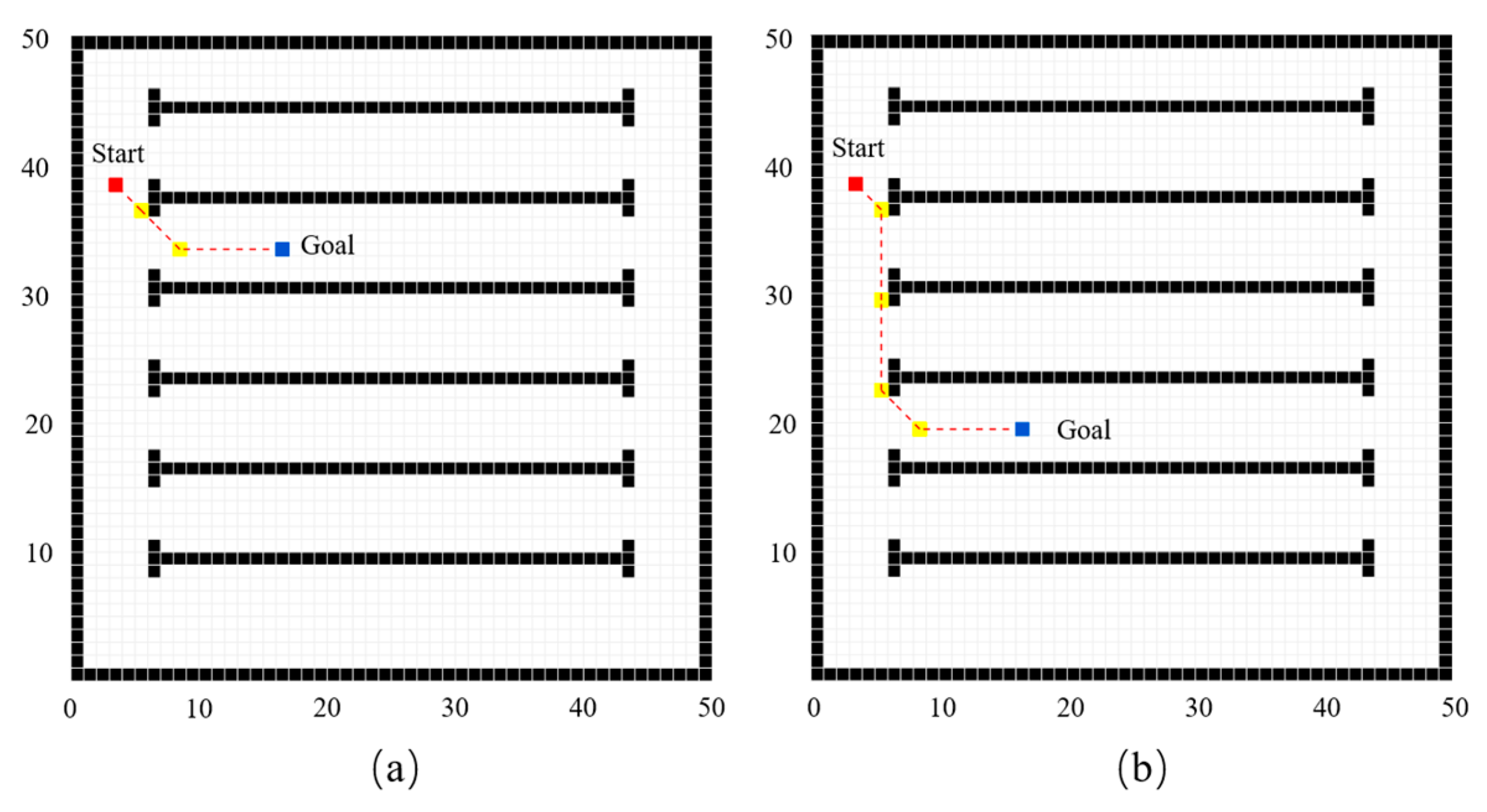
The planned paths generated by the JPS algorithm for setup 1 and setup 2 are illustrated in Figure 8. Figure 8a presents the JPS planning result for setup 1, and Figure 8b presents the corresponding planning result for setup 2.

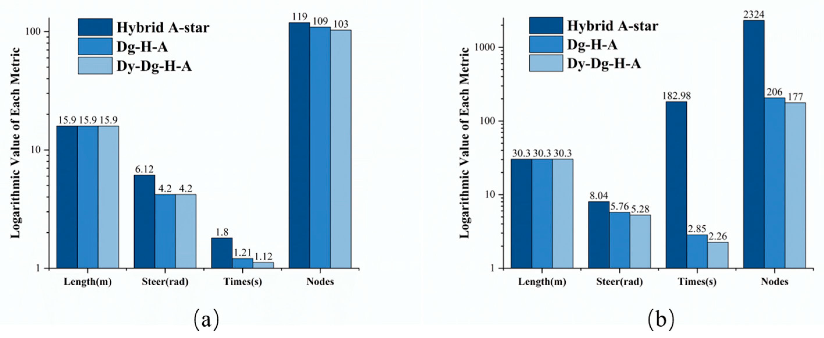
In setup 1, the planned path lengths of the Hybrid A-star algorithm, DG–Hybrid A-star algorithm, and Dy–DG–Hybrid A-star algorithm were all approximately 15.9 m, indicating that the path lengths remained essentially consistent across all three methods. The cumulative steering angles for the Hybrid A-star, DG–Hybrid A-star, and Dy–DG–Hybrid A-star algorithms were 6.12 radians, 4.20 radians, and 4.20 radians, respectively. Compared to the standard Hybrid A-star, both the DG–Hybrid A-star and the Dy–DG–Hybrid A-star algorithms reduced the cumulative steering angle by 31.37%. The computational times for the Hybrid A-star, DG–Hybrid A-star, and Dy–DG–Hybrid A-star algorithms are 1.80 s, 1.21 s, and 1.12 s, respectively. Compared to the Hybrid A-star algorithm, the computational times of the DG–Hybrid A-star and Dy–DG–Hybrid A-star algorithms are reduced by 32.78% and 37.78%, respectively. The number of expanded nodes for the Hybrid A-star, DG–Hybrid A-star, and Dy–DG–Hybrid A-star algorithms was 119, 109, and 103, respectively. Compared to the Hybrid A-star, the number of expanded nodes for the DG–Hybrid A-star and Dy–DG–Hybrid A-star algorithms was reduced by 8.4% and 13.45%, respectively.

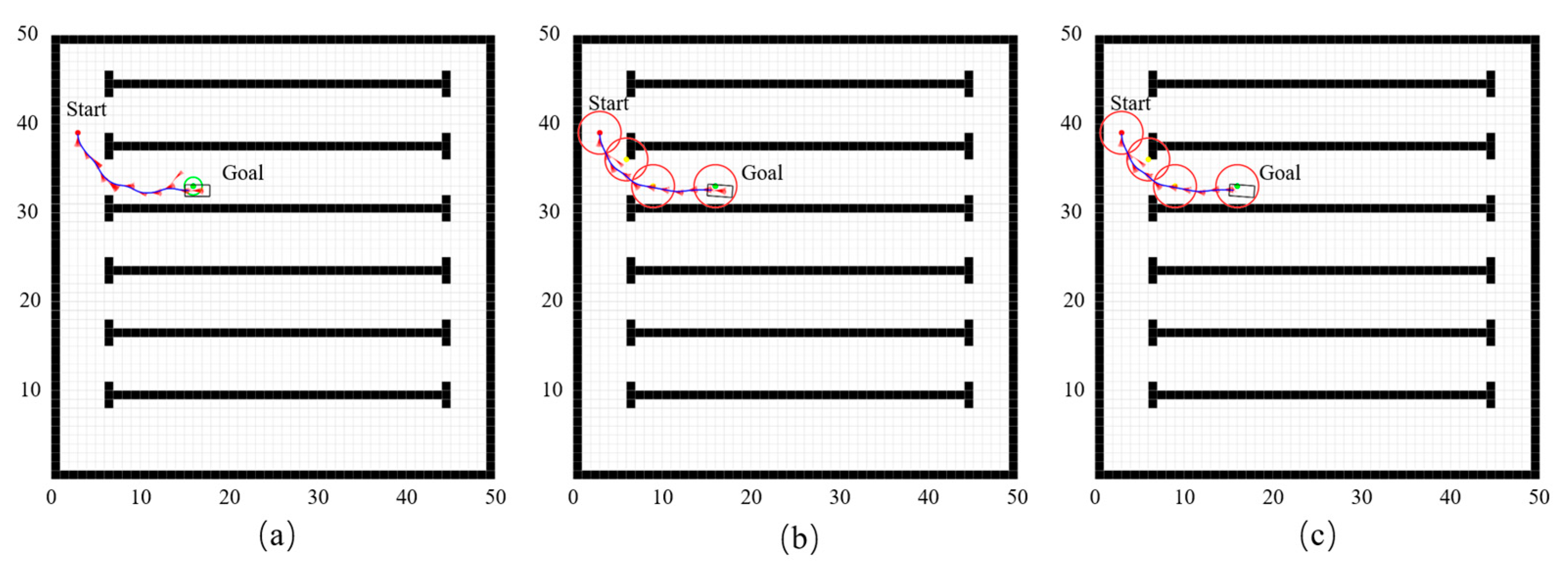
The planned paths under setup 1 for the three algorithms are shown in Figure 9. Figure 9a–c present the results of the standard Hybrid A-star, DG–Hybrid A-star, and Dy–DG–Hybrid A-star algorithms, respectively. In Figure 9, the red dots are the starting points, the green dots are the goal points, the blue solid lines represent the planned paths, and the yellow dots represent the key jump points. The green circles in Figure 9a represent the parking area, while the red circles in Figure 9b,c represent the tolerance radius. The parking criteria of all algorithms are consistent.

To further assess the practical performance of the algorithms under varying conditions, simulations were also conducted using setup 2. In setup 2, the planned path lengths for the Hybrid A-star, DG–Hybrid A-star, and Dy–DG–Hybrid A-star algorithms are all 30.3 m, remaining largely unchanged; The cumulative steering angles for the Hybrid A-star, DG–Hybrid A-star, and Dy–DG–Hybrid A-star algorithms are 8.04 radians, 5.76 radians, and 5.28 radians, respectively. Compared to the Hybrid A-star algorithm, the cumulative steering angles of the DG–Hybrid A-star and Dy–DG–Hybrid A-star algorithms are reduced by 28.36% and 34.33%, respectively. The computational times for the Hybrid A-star, DG–Hybrid A-star, and Dy–DG–Hybrid A-star algorithms are 182.98 s, 2.85 s, and 2.26 s, respectively. Compared to the Hybrid A-star algorithm, the computational times for the DG–Hybrid A-star and Dy–DG–Hybrid A-star algorithms are reduced by 98.44% and 98.76%, respectively. The number of expanded nodes for the Hybrid A-star, DG–Hybrid A-star, and Dy–DG–Hybrid A-star algorithms was 2324, 206, and 177, respectively. Compared to the Hybrid A-star algorithm, the number of expanded nodes for the DG–Hybrid A-star and Dy–DG–Hybrid A-star algorithms was reduced by 91.14% and 92.38%, respectively.

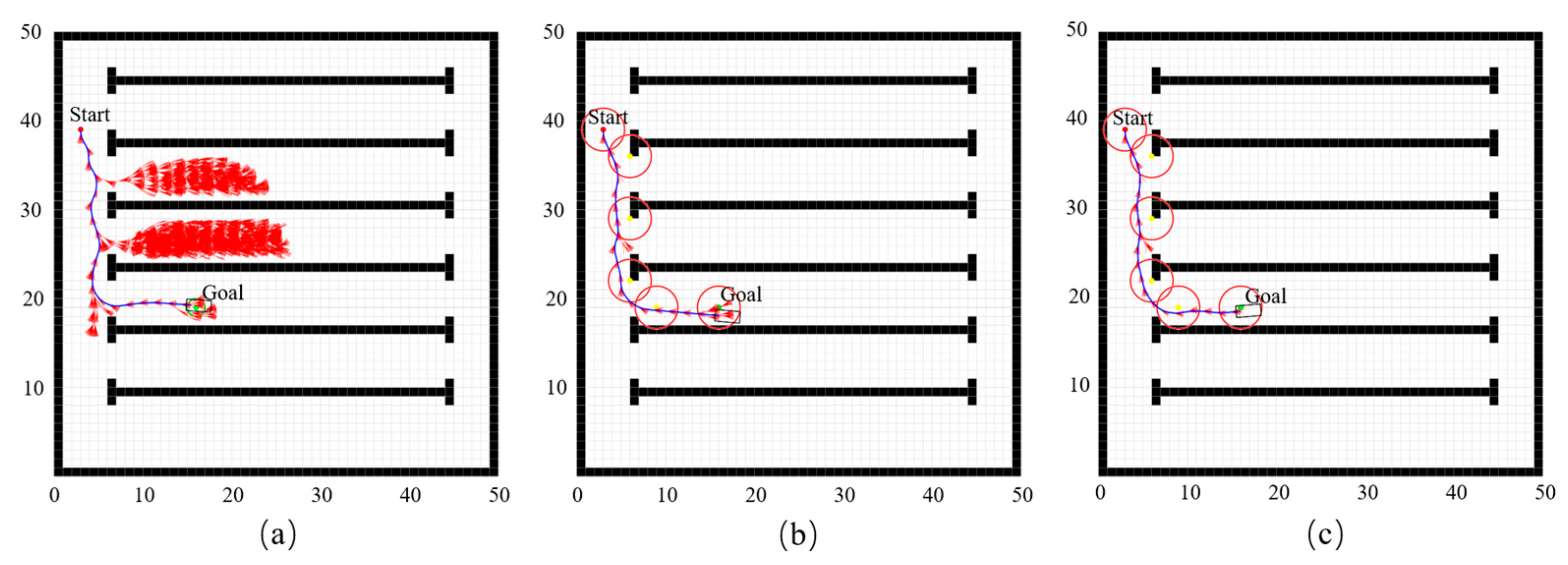
The planned paths under setup 2 for the three algorithms are presented in Figure 10. Figure 10a–c present the paths generated by the standard Hybrid A-star, DG–Hybrid A-star, and Dy–DG–Hybrid A-star algorithms, respectively. The visual elements in Figure 10 follow the same definitions as in Figure 9.

By comparing the path length, cumulative steering angle, computation time, and number of expanded nodes under setup 1 and setup 2, several key conclusions can be drawn. Compared to the original Hybrid A-star algorithm, the proposed DG–Hybrid A-star algorithm significantly reduces redundant node expansions, particularly around U-shaped obstacles, while maintaining a consistent path length. Specifically, DG–Hybrid A-star reduces the cumulative steering angle by 31.37%, computation time by 32.78%, and the number of expanded nodes by 8.4%. In addition, the Dy–DG–Hybrid A-star algorithm, which incorporates segmented heuristic weighting, offers further improvements—reducing computation time by 5% and node expansion by 5.04% compared to the DG–Hybrid A-star.

To more effectively illustrate the comparative performance of key evaluation metrics across the algorithms, both the absolute values and relative improvement rates are illustrated in Figure 11 and Figure 12, respectively. In Figure 11, Dg-H-A represents the DG–Hybrid A-star algorithm, and Dy-Dg-H-A represents the Dy–DG–Hybrid A-star algorithms. In Figure 12a, Dg-H-A improvement represents the improvement rates of the DG–Hybrid A-Star algorithm compared to the Hybrid A-Star algorithm. In Figure 12a, the Dy-Dg-H-A improvement represents the improvement rates of the Dy–DG–Hybrid A-Star algorithm compared to the Hybrid A-Star algorithm. Notably, in Figure 12, as all algorithms produce identical path lengths, only the improvements in the remaining three metrics are evaluated for comparison. The Dy–DG–Hybrid A-star algorithm consistently achieves better performance than the other two methods in terms of steering smoothness, planning efficiency, and search efficiency. In the case of long-distance path planning under setup 2, the DG–Hybrid A-star and Dy–DG–Hybrid A-star algorithms reduce computation time by 98.44% and 98.76%, and the number of expanded nodes by 91.14% and 92.38%, respectively, highlighting the enhanced scalability of the proposed approach.

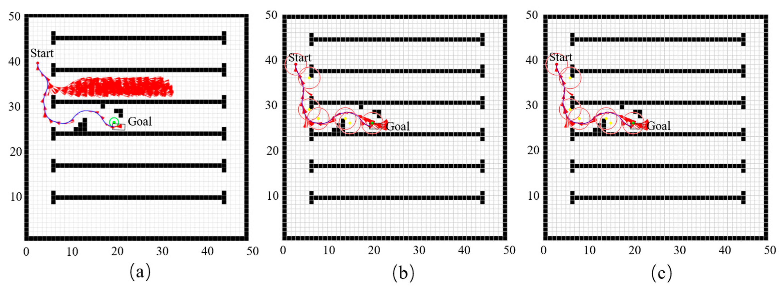
To further investigate the performance of the proposed algorithm in complex environments and verify its feasibility and stability under realistic conditions, additional obstacles were introduced into the original map to create a more challenging scenario. For this environment, the path planning results of the Standard Hybrid A-Star algorithm, JPS algorithm, DG–Hybrid A-Star algorithm, and Dy–DG–Hybrid A-Star algorithm are summarized in

Table 4. Path Planning Performance Comparison in Complex Environments.

Indexes	Hybrid A-Star	DG–Hybrid A-Star	Dy–DG–Hybrid A-Star
Planned path length (m)	30.7	30.7	30.7
Sum of steering angle changes (rad)	8.02	6.36	6.48
Computational time (s)	182.37	6.81	6.53
Expanded node count	1727	272	270

.

As shown in the results, the DG–Hybrid A-Star algorithm significantly reduces computational time, cumulative steering angle change, and the number of expanded nodes compared with the standard Hybrid A-Star algorithm. Furthermore, the Dy–DG–Hybrid A-Star algorithm, building upon DG–Hybrid A-Star, achieves further reductions in computation time and node expansion. However, a slight increase in the cumulative steering angle change is observed.

This increase is likely due to the frequent switching of dynamic heuristic coefficients during turning-intensive segments, which may cause some intermediate node expansions to be skipped, resulting in a larger overall steering angle accumulation.

To evaluate the path planning performance of different algorithms in complex environments, four methods were tested under the same obstacle configuration: the Standard Hybrid A-Star algorithm Figure 13a, the DG–Hybrid A-Star algorithm Figure 13b, and the Dy–DG–Hybrid A-Star algorithm Figure 13c.

4. Conclusions

To enhance the planning efficiency of the Hybrid A-star algorithm in structured agricultural environments, such as greenhouses with elongated U-shaped obstacles, this study introduced an enhanced Hybrid A-star path planning method that combines directional guidance and a segmented heuristic weighting strategy. This method mitigates the problem of redundant node expansion near elongated obstacle regions. The proposed method first uses the JPS algorithm to extract key waypoints, which serve as directional references for guiding node expansion in the Hybrid A-star algorithm. Simulation results show that the DG–Hybrid A-star algorithm, which combines directional guidance, significantly reduces the number of expanded nodes and enhances both path smoothness and planning efficiency compared to the standard Hybrid A-star.

To further improve path planning efficiency and smoothness, a segmented heuristic weighting mechanism was introduced, yielding the Dy–DG–Hybrid A-star algorithm. This mechanism dynamically adjusts the heuristic weight based on path segment type, accelerating search along straight paths while preserving curvature continuity in turning segments. Comparative experiments across various scenarios demonstrate that the Dy–DG–Hybrid A-star algorithm consistently achieves lower cumulative steering angles, fewer expanded nodes, and faster computation times, validating its superior efficiency and robustness in structured agricultural settings.

The proposed Dy–DG–Hybrid A-star algorithm integrates directional guidance with a segment-based dynamic heuristic strategy, which significantly reduces redundant node expansion and computation time while maintaining high path smoothness. However, the algorithm’s performance still depends on the quality of the JPS-generated reference path and is primarily applicable to static or semi-structured environments. In future work, we plan to extend the algorithm to handle dynamic obstacles and incorporate motion prediction models, thereby improving its robustness and adaptability in real-world agricultural scenarios.