A Novel WaveNet Deep Learning Approach for Enhanced Bridge Damage Detection

Abstract

Bridges are vital components of global infrastructure, with millions constructed over the years. Many of them face aging and are vulnerable to risks. Traditional bridge inspection methods are costly and time-consuming. They often rely on many manual laborers without providing system-level insights. Moreover, these outdated approaches make it difficult to obtain a clear representation of the current bridge health. This paper introduces a novel framework based on deep learning (DL) for identifying local bridge damage using acceleration data collected by Unmanned Aerial Vehicle (UAV)-mounted sensors. The framework employs WaveNet, which was designed as a generative audio DL model. Its causal dilated convolution deals with long-range temporal correlations without recurrence. Two WaveNet regressors are used to predict the damage location and its severity. The methodology is integrated with an optimized sensor spacing strategy for UAV deployments. The results demonstrate that the severity model achieved an average R² = 0.98, while the location model reached R² = 0.85. Optimal sensor spacing “S” was found at S = 1.0 m for localization and S = 0.5 m for severity. A field-simulated case was accurately identified by the two models, representing the potential of the proposed framework for more reliable bridge health monitoring.

1. Introduction

Bridges are important structures that play an effective role in transportation infrastructure. It is essential to keep them safe and running effectively [1]. The backbone of bridge decision-making is still based on periodic visual inspections, which are useful but subjective and inconsistent across inspectors. They rarely provide network-level insight for managing thousands of assets simultaneously [2].

Structural Health Monitoring (SHM) is known as a transformative solution, which offers condition-based rather than time-based maintenance [3]. By using sensors along with analytics, SHM systems can estimate deterioration and support decision-making [4,5]. However, the scalability of SHM for large bridge networks remains unlimited. Deploying dense sensor networks introduces high costs in hardware, communication, and data management, while top constraints such as long-term power reliability and network longevity still exist [6,7,8].

Data volume is another practical hurdle. For example, a single accelerometer channel sampled at 200 Hz with 16-bit resolution produces approximately 34 MB/day (12.6 GB/year) by straightforward calculation; dozens or hundreds of channels per bridge push owners toward “big data” pipelines for storage, processing, and interpretation [9]. Accordingly, data management is considered a core challenge in SHM [10,11].

Consequently, DL has gained significant attention in SHM as a data-driven approach capable of learning informative representations directly from raw signals [12]. Deep neural models like Recurrent Neural Network (RNN), Convolutional Neural Network (CNN), Long Short-Term Memory (LSTM), and Gated Recurrent Unit (GRU) architectures have shown success in pattern recognition, vibration analysis, and anomaly detection [13]. RNNs generate hidden states to model temporal dependence but have limitations with long-range context because of vanishing gradients [14]. The LSTM model is widely used for controlling information flow, making it better than RNNs [15]. The GRU has fewer gates than LSTM and has the same accuracy, which makes it easier and faster to train [16,17]. One-dimensional CNNs learn time series as temporal patterns, which can be strong for classification and vibration signal detection [18,19,20]. Nevertheless, the application of DL models in bridge monitoring has been limited by computational limitations and difficulty of modeling long-temporal dependencies in high-frequency data [21].

Recent advances in UAV techniques have accomplished rapid structural evaluation of civil infrastructure, including bridges [22,23]. UAVs equipped with sensors are being developed to monitor civil infrastructure instead of stationary sensors.

Two types of damage could be found in bridges: local damage and global damage. Local damage, which is studied in this paper, is defined as defects that happen in specific elements of the bridge superstructure. These may include cracks, corrosion, or any kind of local deformation [24,25,26]. On the other hand, global damage alters the overall performance and stability, such as foundation settlement, scour, or bearing deterioration [27,28].

This paper introduces a novel data-driven approach for identifying local bridge damage from UAV-mounted sensor data using DL. The damage is predicted with a pretrained WaveNet model, which was originally developed for speech recognition and audio generation [29]. WaveNet employs causal dilated convolutions that efficiently capture long-range temporal dependencies through sequential processing, which leads to faster training and stable convergence, as demonstrated in similar SHM applications [30]. The dataset involves the relationship between acceleration and time at different damage locations. As shown in Figure 1a, acceleration data exhibits localized changes when a crack is present. These changes are like perturbations in sound waves (Figure 1b). According to this similarity, we adapt two WaveNet regressors to the structural domain and use them to predict damage location and severity from acceleration signals.

WaveNet is applied through different applications related to sound generation. Parallel WaveNet is used in Google Assistant, enabling high-speed speech recognition faster than before [31]. This model is also implemented as an autoencoder, which learns timbre embeddings and generates realistic instrument notes [32]. It has also been used in speech enhancement [33] and electroencephalogram (EEG) signal forecasting [34]. The model has also been used in other fields of expertise, like water wave height prediction in oceans [35] and heart sound classification in biomedical acoustics [36]. WaveNet’s architecture was used in electric load forecasting as an encoder and decoder for national-scale 24 h-ahead demand prediction [37].

In structural engineering, the application of WaveNet is still limited but growing. Ning et al. [38] used the WaveNet model and two other DL models for predicting seismic response. The results showed that WaveNet had competitive accuracy with reduced computation time. Mariani et al. [39] used WaveNet in linear regression to predict structure response using temperature readings. The similarity between sound waves and temperature reading allowed them to apply this model as proposed in this research. In SHM, the model was used as an autoregressive forecaster of structural response by obtaining bridge strain data [40]. WaveNet was tested on Z24 bridge vibration data as a damage classifier. The results showed state-of-the-art accuracy with a smaller model and lower computation time [41]. Mariani et al. [30] used ultrasonic waves as a training dataset for WaveNet to predict damage. WaveNet outperformed other models even without performing any kind of feature engineering. The model had a robust detection when the dataset included some shifts and significant changes.

Despite these studies, WaveNet has not yet been fully explored for vibration-based bridge damage detection using time-series acceleration data. Its combination of long-range dependency modeling, computational efficiency, and robustness to temporal shifts makes it particularly well suited for UAV-based SHM systems. This paper extends the WaveNet framework into the bridge engineering domain while integrating it with a UAV sensor network and an optimized sensor spacing strategy for real-world applications.

Beyond damage prediction, the framework also addresses sensor layout. We investigate optimal spacing for UAV-mounted sensors and demonstrate a three-sensor setup as a practical proof of concept [42], while noting that the method scales to any number of sensors.

To train the model, a dataset is generated via a forced vibration analysis on a bridge [43,44,45,46]. An inspection vehicle traverses the span while UAV-mounted sensors record the response [47]. The vehicle may be human-driven or autonomous (e.g., driverless platforms), enabling repeatable data collection even when post-event conditions complicate access. The resulting time series are used to train WaveNet. During inference, field measurements from the sensor configurations are passed to the pretrained model to output predicted damage location and severity (see Figure 2).

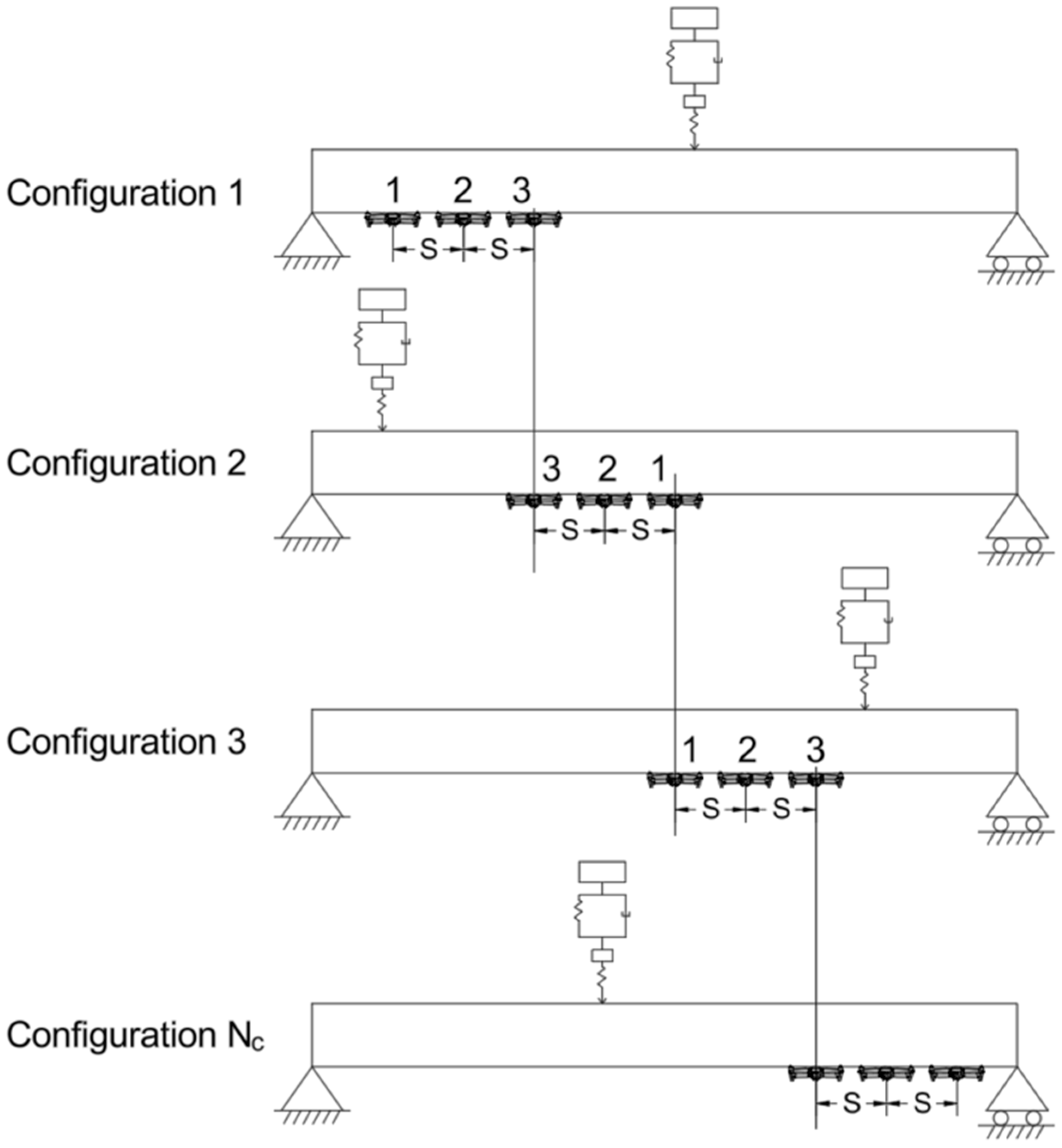
For data collection in practice, the orchestrated UAV concept is introduced with optimum sensor spacing “S” to achieve full-span coverage efficiently [48,49]. As shown in Figure 3, the inspection proceeds through a sequence of configurations. Starting near one abutment (Configuration 1), three sensors (1, 2, 3) record while the vehicle crosses. Then, sensor 3 is held in place while the others advance by “S” (Configuration 2). The process repeats (Configuration 3, …) with sensors moving forward to maintain spacing until the final configuration N_c reaches the far end. This controlled inspection preserves the target spacing, ensures complete coverage, and supplies the model with consistent input for robust localization and severity estimation.

The following sections are structured as follows: Section 2 explains the bridge studied and sensor characteristics. Section 3 describes the methodology and dataset generation. Section 4 presents the analysis results. Finally, Section 5 and Section 6 explain the summary and conclusion. The acronyms used in this paper are summarized in Appendix A (

Table A1. List of acronyms.

Acronym	Definition	Acronym	Definition
1-D	One-Dimensional	API	Application Programming Interface
CNN	Convolutional Neural Network	DL	Deep Learning
EEG	Electroencephalogram	FE	Finite Element
GB	Gigabyte	GRU	Gated Recurrent Unit
LSTM	Long Short-Term Memory	MAE	Mean Absolute Error
MEMS	Micro-electromechanical System	NumPy	Numerical Python
RC	Reinforced Concrete	ReLU	Rectified Linear Unit
RNN	Recurrent Neural Network	SD	Standard Deviation
SHM	Structural Health Monitoring	SWA	Stochastic Weight Averaging
TLA	Temporal Laplacian Acceleration	UAV	Unmanned Aerial Vehicle

).

2. Bridge and Sensor Description

The bridge considered in this study is a reinforced concrete (RC) whose structural system is a simply supported beam, representing a typical short-span bridge. The RC beam has a rectangular cross-section with a depth of 0.9 m and width of 0.3 m. The span is 10 m, and the RC density is 25 kN/m³. The elasticity modulus E is 30 GPa. The structural system of the bridge studied is shown in Figure 4.

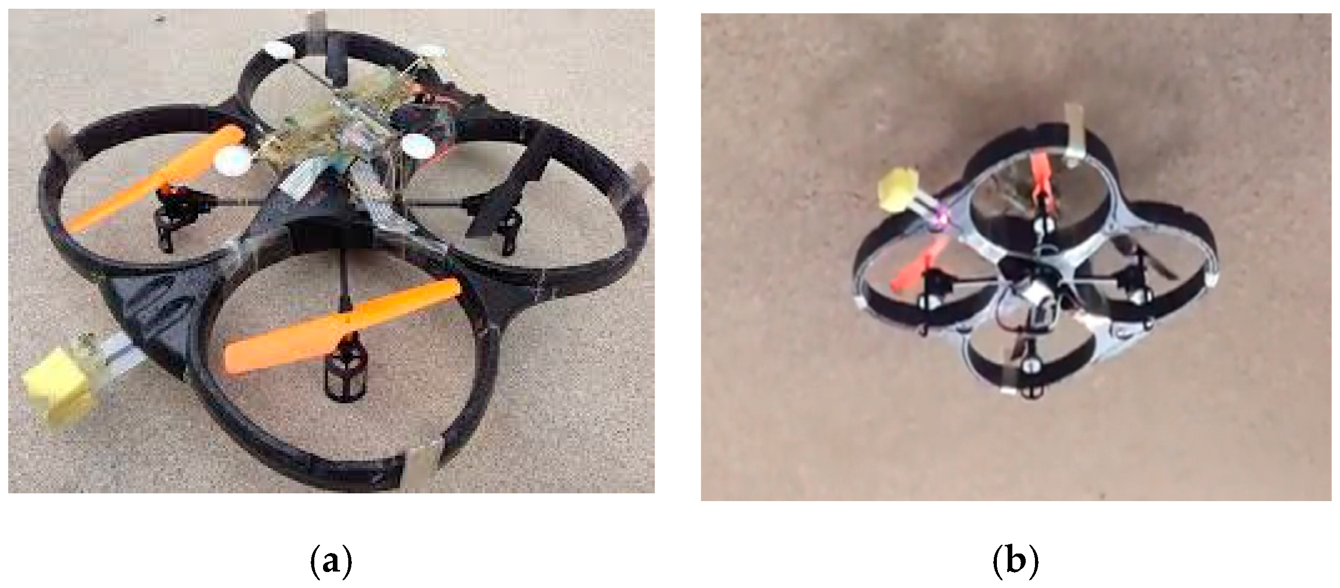
For vibration measurements, the framework utilizes UAVs equipped with sensors, which are high-precision triaxial micro-electromechanical (MEMS) accelerometers. Each sensor operates at a sampling frequency of 5 kHz to ensure accurate capture of dynamic responses. Each UAV can be equipped with a passive perching mechanism that enables it to temporarily attach to the bridge surface for a short period (<5 min). The mechanism employs directional dry adhesives and micro-spine tendons to grip vertical or inverted surfaces, allowing secure contact for vibration sensing, while minimizing noise from UAV dynamics [50,51]. Figure 5 illustrates the UAV setup and mounted accelerometer configuration.

3. Methodology

3.1. Proposed Framework

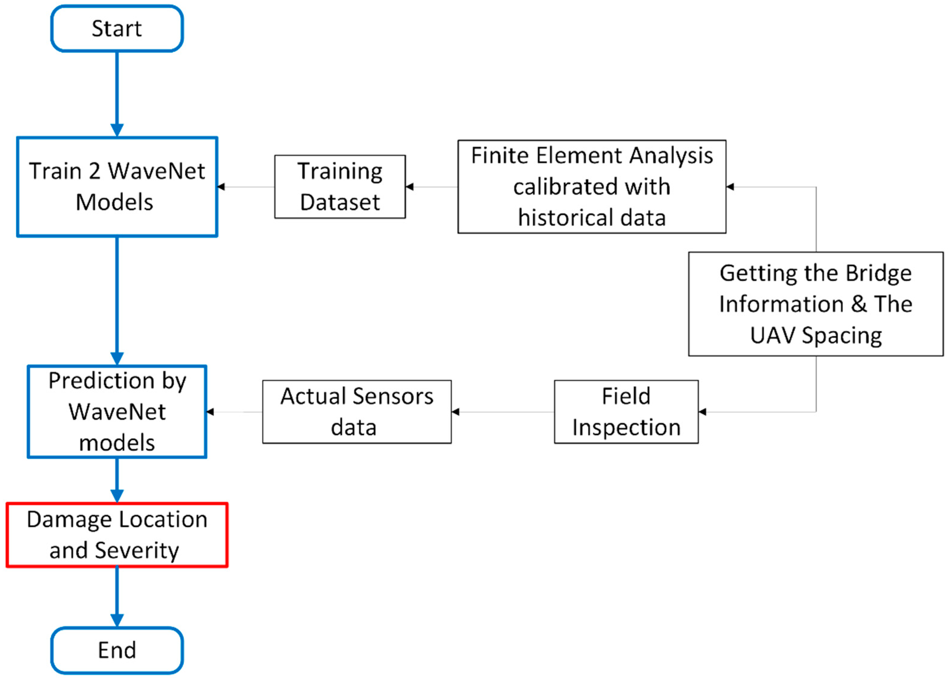
The steps of the framework used are illustrated in Figure 6. The bridge information is obtained from old design data or initial inspection. The information of the current bridge studied in this paper is described in the previous section. Based on this information, the FE analysis is carried out to generate the training dataset. The analysis is based on hypothetical cases of damage to the same bridge studied. If a historical dataset is also available, it can be used to calibrate the analysis model while generating training cases. Then, the WaveNet models are trained based on this data and with respect to the selected UAV-mounted sensor spacing “S.” At the same time, a field inspection is performed by using the abovementioned orchestrated UAV-mounted sensors concept with the same spacing “S.” Then, the actual sensor data are passed to the pretrained WaveNet models to predict the damage location and severity on the bridge. The field data are simulated as a case that has a predefined damage at a location of 5 m and 15% severity using three UAV-mounted sensors.

The WaveNet-based framework is implemented in Python 3.12.5. Different libraries are used within this framework, such as Numerical Python (NumPy) 2.2.3 [52] for matrix mathematical operations, Pandas 2.2.3 [53] for loading individual data files, PyTorch 2.7.1 [54] for loading and rearranging all the data into matrices, and Matplotlib 3.10.1 [55] for plotting training curves for the models.

3.2. Dataset

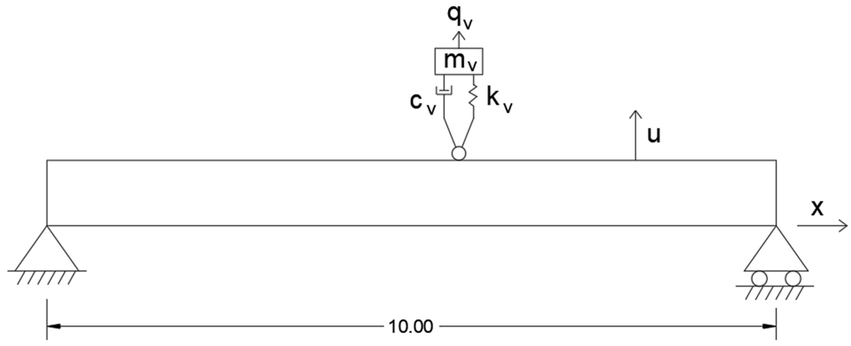
The dataset consists of Finite Element (FE) simulations of the RC bridge studied. The FE analysis was carried out to generate a dataset for training the WaveNet models. This analysis was conducted using a vehicle–bridge interaction model [56]. Acceleration responses are produced by the analysis at intervals of 0.1 m along the bridge. These interval points are assumed to be the places of available UAV-mounted sensors. These intervals balance practical deployment and computational efficiency. A quarter-car model is utilized as a moving load in this analysis to obtain the bridge response, as shown in Figure 7 [43,44,45].

Each case has nine damage locations from 1 m to 9 m. Each location has nine damage severities, with a range from 10% to 90%. Accordingly, 81 damage cases are generated from the FE analysis in addition to the undamaged case. Therefore, the total number of cases considered in this training dataset is 82 cases. Figure 8 shows a general representation of the damaged location in all the cases of this data.

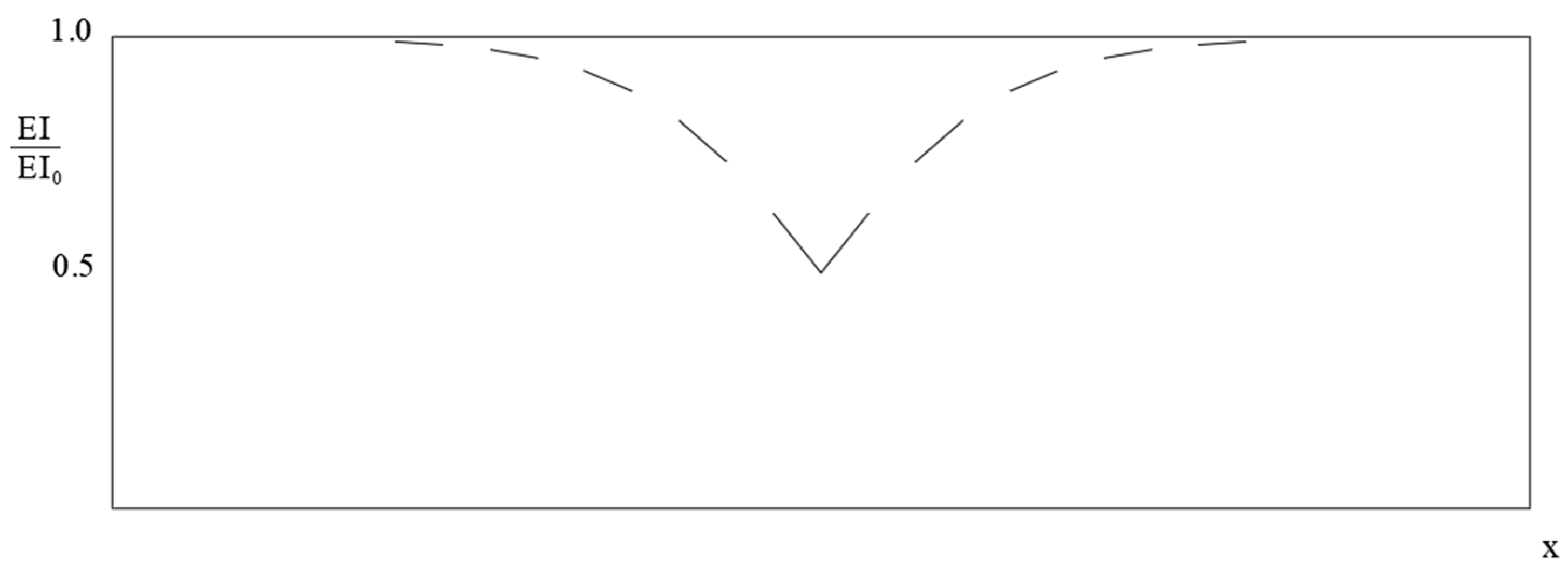
The damage representation in the FE analysis follows the exponential flexural stiffness reduction model proposed by Christides and Barr [57]. The corresponding reduced stiffness is expressed through the following equation.

$$\mathrm{E}\mathrm{I}\left(\mathrm{x}\right)={\displaystyle \frac{\mathrm{E}{\mathrm{I}}_0}{1+\left(\frac{{\mathrm{I}}_0}{{\mathrm{I}}_{\mathrm{r}}}-1\right)e^{\frac{-4\mathsf{\alpha }\left|\mathrm{x}-{\mathrm{x}}_{\mathrm{i}}\right|}{\mathrm{d}}}}}$$

(1)

EI₀ denotes the flexural stiffness of the beam in its uncracked condition, while EI(x) represents the stiffness at any given location x due to the presence of a crack. The terms I₀ and I_r correspond to the moments of inertia of the beam for the uncracked and cracked sections, respectively. The variable x_i indicates crack location, d is the depth of the beam section, and α is a dimensionless constant used to estimate the degree of the stiffness reduction caused by the crack.

Experimental work initially estimated α to be 0.667 for mid-span cracks. However, Shen and Pierre [58] later recommended a value of 1.936. Consequently, Shen and Pierre [59] proposed this value to be taken as 1.276 for a beam with a single-edge crack. In this paper, α = 1.276 is adopted for the studied rectangular beam section.

Damage severity is defined as the ratio between the flexural stiffness at the crack location and the original (uncracked) stiffness [60,61] as follows:

$$\mathrm{S}\mathrm{e}\mathrm{v}\mathrm{e}\mathrm{r}\mathrm{i}\mathrm{t}\mathrm{y}={\displaystyle \frac{\mathrm{E}{\mathrm{I}}_0-\mathrm{E}{\mathrm{I}}_{\mathrm{r}}}{\mathrm{E}{\mathrm{I}}_0}}\times 100$$

(2)

The flexural stiffness change at the crack location is illustrated in Figure 9 with a 50% reduction. It is worth noting that there are other models used to represent the crack such as the linear stiffness reduction model [62] and the rotational spring model [63].

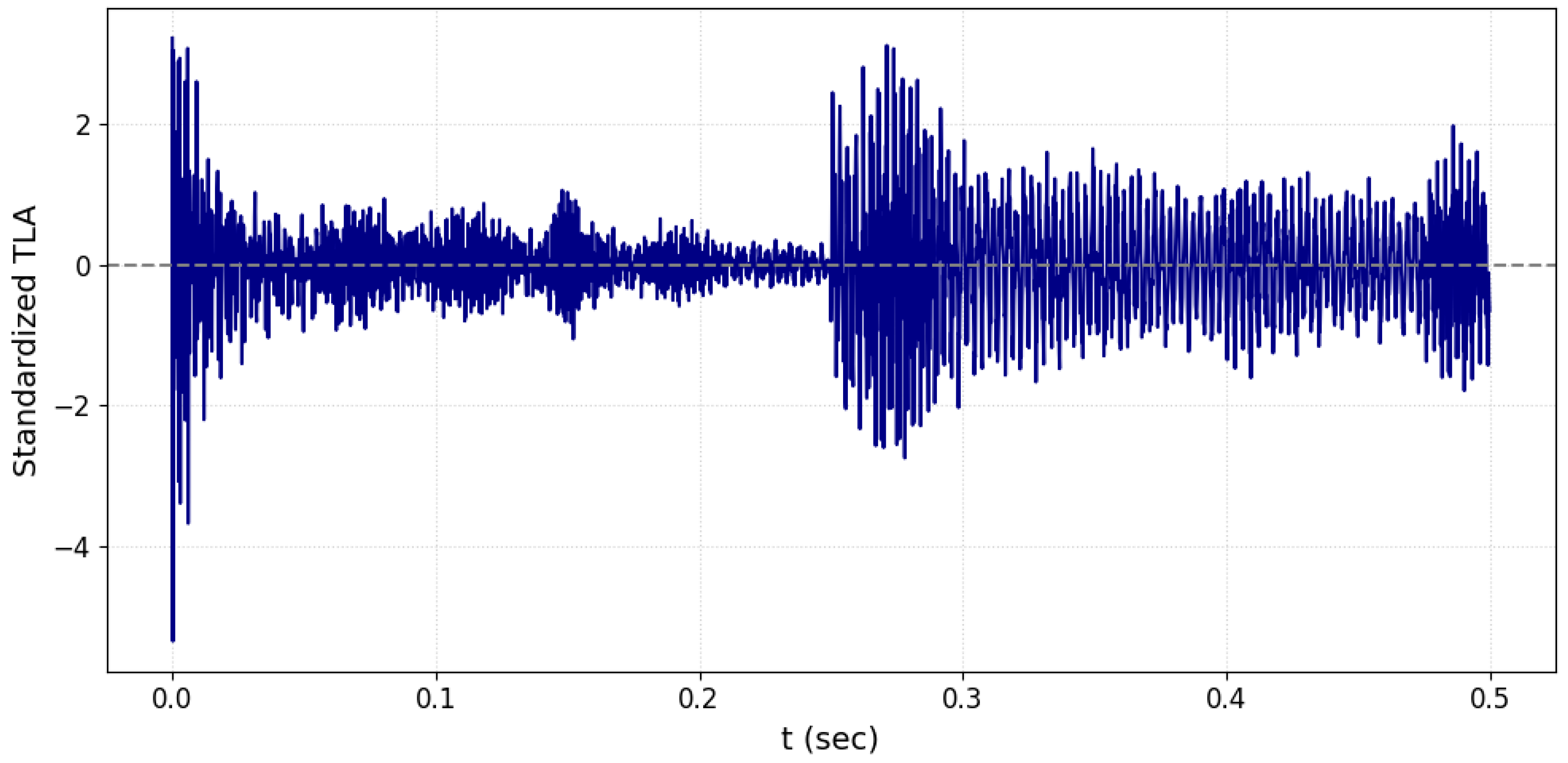
It is noted that all the raw accelerations from these cases had minimal values. Therefore, Temporal Laplacian Acceleration (TLA) is calculated to represent larger values so that the model can differentiate among each other and train smoothly. The Laplacian operator is defined as the divergence of the gradient of a function in Euclidean space. It is calculated by summing the second derivatives with respect to the independent variable for functions expressed in Cartesian coordinates [64,65]. In this study, acceleration is a time-dependent variable. This means that the TLA is calculated as the second derivative of the acceleration with respect to time as follows:

$$\mathrm{T}\mathrm{L}\mathrm{A}\cong {\displaystyle \frac{{\mathrm{a}}_{\mathrm{t}-∆\mathrm{t}}-2{\mathrm{a}}_{\mathrm{t}}+{\mathrm{a}}_{\mathrm{t}+∆\mathrm{t}}}{{∆\mathrm{t}}^2}}$$

(3)

where a_t–Δt, a_t, and a_t+Δt are the accelerations at three successive time steps, and Δt is the step length. For UAV-mounted sensors operating at a sampling frequency of 5 kHz, the step length is defined as Δt = 1/5000 = 0.0002 s, ensuring that the discrete Laplacian computation aligns with the sensor’s sampling rate.

The FE analysis yields a multichannel one-dimensional (1-D) time series consisting of time and sensors. WaveNet models consume this data as 1-D sequences over time, with sensor positions provided as parallel input channels (shaped as channels x time). To ensure consistent training, each channel is then standardized using training-only statistics (mean, standard deviation) to avoid data leakage and ensure proper scaling across splits [66]:

$${\mathrm{X}}_{\mathrm{s}\mathrm{t}\mathrm{d}}={\displaystyle \frac{\mathrm{X}-\mathsf{\mu }}{\mathrm{S}\mathrm{D}}}$$

(4)

where $\mathsf{\mu }$ and $\mathrm{S}\mathrm{D}$ are the channel mean and standard deviation, respectively. Figure 10 illustrates one example (damage at 5 m, severity 50%) after channel-wise standardization for only one channel from a sensor at position 3 m.

The target values for the location range from 0 to 10, and the severity is from 10% to 90%. Therefore, the target values are normalized from 0 to 1 as follows:

$${\mathrm{X}}_{\mathrm{n}}={\displaystyle \frac{\mathrm{X}-\mathrm{m}\mathrm{i}\mathrm{n}}{\mathrm{m}\mathrm{a}\mathrm{x}-\mathrm{m}\mathrm{i}\mathrm{n}}}$$

(5)

3.3. UAV Sensor Deployment

The field data are collected using the orchestrated drones concept explained in the introduction. The UAV-mounted sensors are placed across all configurations with constant spacing “S” among them. The first configuration starts near the beginning of the bridge. Consequently, the concept is applied until reaching the last configuration at the bridge to obtain the actual sensor data. The sensors have a frequency of 5 kHz, which means that acceleration readings are taken in each sensor every 0.0002 s till the vehicle leaves the bridge. Then, the corresponding TLA values for the accelerations are estimated as mentioned previously. Given the actual sensor data and training dataset, WaveNet models can be trained to predict the current damage scenario effectively using different “S” values.

However, the orchestrated drones concept has some practical challenges. The main ones among these are limited battery endurance and environmental conditions such as wind turbulence. To address these challenges, UAV deployment can employ high-capacity batteries and on-site or vehicle-mounted charging pads to extend inspection time [67]. For longer bridges, a spare battery exchange system allows uninterrupted inspection cycles. Moreover, the perching mechanism, as mentioned in Section 2, enables UAVs to land securely on the bridge surface, mitigating the effects of wind and ensuring stable data acquisition. These improvements enhance the feasibility of orchestrated UAV inspection in real-world bridge environments.

3.4. WaveNet Models

WaveNet is a 1-D time series model that was implemented to train on audio waves. It was used to predict and generate audio waves as a state-of-the-art model [29]. They factored the product conditional probability by the joint probability of waveform $\mathrm{x}=\left\{{\mathrm{x}}_1,\dots ,{\mathrm{x}}_{\mathrm{T}}\right\}$ as follows:

$$\mathrm{p}\left(\mathrm{x}\right)=\prod _{\mathrm{t}=1}^{\mathrm{T}}\mathrm{p}\left({\mathrm{x}}_{\mathrm{t}}\right|{\mathrm{x}}_1,\dots ,{\mathrm{x}}_{\mathrm{t}-1})$$

(6)

A stack of convolutional layers models the conditional probability distribution [29]. The network does not have any pooling layers. This model is mainly used to produce one output as it is a 1-D model. However, many trials in this paper are carried out using two outputs. The results did not show significant improvement until using one output. Therefore, two models are used for this paper: the first for the prediction of damage severity, and the second for the prediction of damage location. The same training datasets are used for both models.

3.4.1. Severity Model

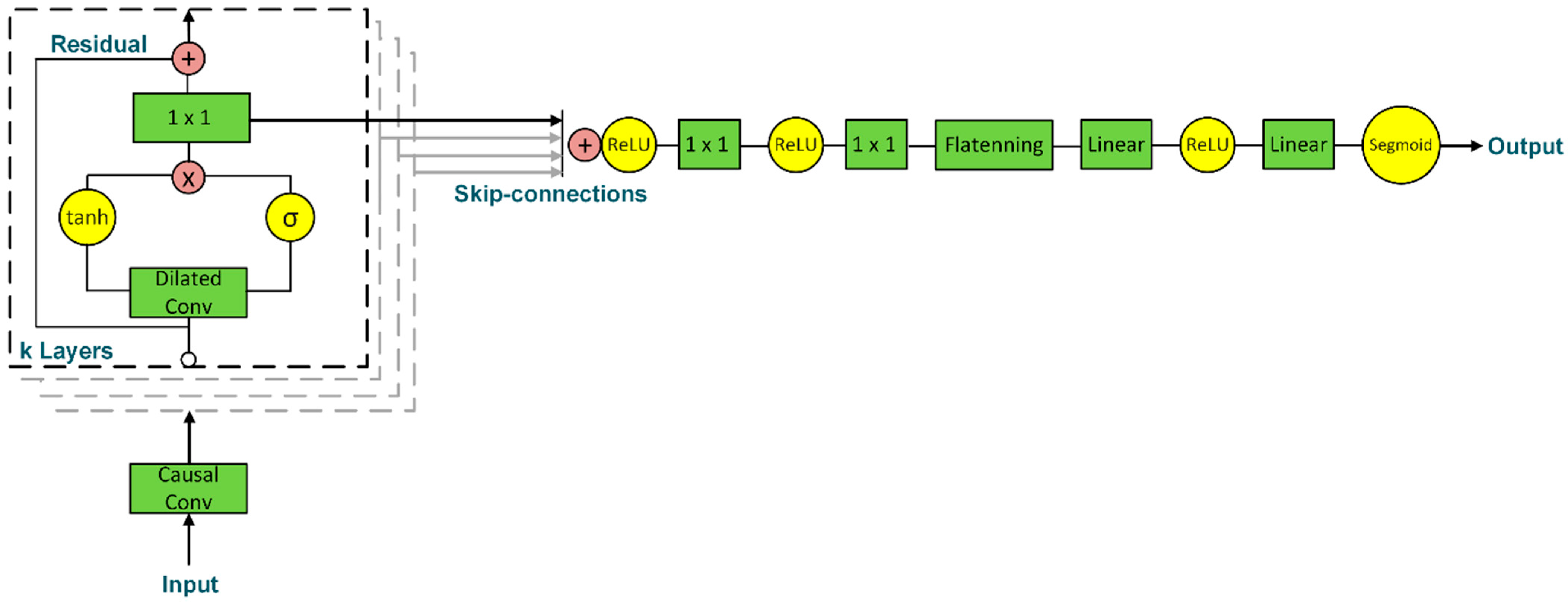
The architecture used for the severity model is shown in Figure 11. The severity model detects damage severity based on TLA values, so it has an easier architecture than the upcoming location model. The original model had a different stage right before the output, as it was used for classification. This stage was changed to a flattening layer, then a linear layer, as the bridge studied is a regression problem.

The model begins with the input channels, which represent the number of features for a single time step. This determines the shape of the input tensor. In our case, the sensor feature per time step depend on the number of UAV-sensor points used based on their spacing “S”. For example, if the spacing among UAV-sensors is 0.1 m for the 10 m bridge span, the UAV-sensors used as channels are 99, neglecting the supports. The spacing cases used in this paper are 2 m, 1 m, 0.5 m, 0.3 m, and 0.1 m for a 10 m bridge. This means that the number of input channels for these cases is 4, 9, 19, 33, and 99, respectively.

After receiving the input, the model passes through an advanced neural network, which is called causal convolution. Regarding the standard Convolutional Neural Network, the inputs depend on the past, present, and future input neurons, as shown in Figure 12a. However, the causal Convolutional Neural Network in WaveNet works with a new technique such that input neurons depend only on the present and the past neurons, not the future ones, as shown in Figure 12b.

After causal convolution, the outputs enter the residual block. According to the WaveNet architecture in Figure 11, a residual block is a modular unit that applies nonlinear transformations and processes the input. By avoiding vanishing gradients, the block uses residual connections to aid in training deep networks. The residual block depends on hyperparameters that must be defined accordingly, such as kernel size, stack size, and layer size.

The number of filters employed in the time-based dimension is known as the kernel size. Though they cost more to compute, larger kernels capture more training. Stack size is the number of times a set of residual blocks is repeated. Stacking residual blocks increases the model’s capacity to learn more complex temporal relationships while maintaining skip connections to avoid vanishing gradients.

The number of residual blocks in one stack is called the layer size. By increasing the layer size, the model will increase another factor called the receptive field, which is the number of inputs that affect a single output. A larger layer size increases the receptive field, which helps the model learn patterns over longer time periods. The receptive field depends on the kernel size, dilations, layer size, and stack size. In our model, it is calculated as follows:

$$\mathrm{R}\mathrm{e}\mathrm{c}\mathrm{e}\mathrm{p}\mathrm{t}\mathrm{i}\mathrm{v}\mathrm{e} \mathrm{f}\mathrm{i}\mathrm{e}\mathrm{l}\mathrm{d}=1+\left(\mathrm{k}\mathrm{e}\mathrm{r}\mathrm{n}\mathrm{e}\mathrm{l} \mathrm{s}\mathrm{i}\mathrm{z}\mathrm{e}-1\right)[1+\mathrm{s}\mathrm{t}\mathrm{a}\mathrm{c}\mathrm{k} \mathrm{s}\mathrm{i}\mathrm{z}\mathrm{e}(2^{\mathrm{l}}-1\left)\right]$$

(7)

This concept is closely linked to dilated convolution, which is another key feature of WaveNet. The data passes through it after entering the residual block. The main target of this stage is to make the output infected with a higher number of inputs from a wide range of input locations. Dilation means extending the causal convolution by adding gaps (dilations) between filter elements, effectively increasing the receptive field without increasing the number of parameters, as shown in Figure 13. When the receptive field is increased, the output will be more reliable to the inputs. The dilation in this research is assumed to be $2^{\mathrm{l}}$ where $\mathrm{l}$ is the current hidden layer number.

Consequently, the model in the following stage after convolution relies on the following activation function:

$$\mathrm{z}=\tanh {(\mathrm{W}}_{\mathrm{f},\mathrm{k}}\ast \mathrm{x})\odot \mathsf{\sigma }{(\mathrm{W}}_{\mathrm{g},\mathrm{k}}\ast \mathrm{x})$$

(8)

where k is the layer index, f and g are the filter and gate, σ is the sigmoid function, * is the convolutional operator, and ⊙ is the element-wise multiplication. The learner filter is W. Batch normalization is applied at the end of dilated causal convolution to normalize activations based on the mean and variance calculated across the batch. This operation works well with large batch sizes but can be unstable with small batch sizes. For this shallower severity model, which uses consistent batch sizes and a short receptive field, batch normalization is sufficient and computationally efficient.

After that, the data passes through a standard 1 × 1 convolution to begin the residual stage. In this stage, the processed output is combined with the input, which is defined as residual channels. This residual connection ensures that the original input signal is preserved and allows deeper layers to focus on learning additional features rather than recomputing the same ones.

Then, the network can efficiently incorporate features from all residual blocks thanks to skip connections. They offer an extra channel for information to go across layers. Skip connections help accumulate features from all layers for the final output. They enable the model to train efficiently by improving gradient flow during backpropagation. The output from the residual block through the skip connections is defined as skip channels, whose number could be defined as the number of features output from the block and sent to the skip connections. This describes the number of channels the skip connections produce, which are passed into the next Rectified Linear Unit (ReLU) activation function. This establishes how much information the model reproduces forward and the dimensionality of the output before the skip connections.

Accordingly, the data passes twice through the ReLU activation function and the standard Convolutional Neural Network. Finally, the data is passed through a flattening layer and then a linear layer. The flattened layer is placed to prepare the output by reshaping multidimensional tensors into a single vector, ensuring compatibility with the fully connected layers. In WaveNet, the flattening layer prepares the network’s high-dimensional features (e.g., from residual/skip connections) for the final linear output layer. The linear layer acts as a fully connected layer that directly predicts the continuous target values. Each output neuron corresponds to a single regression target. It maps the flattened features to the desired number of continuous output values. The linear layer computes as follows:

$$\mathrm{y}=\mathrm{W}\mathrm{x}+\mathrm{b}$$

(9)

where $\mathrm{W}$ and $\mathrm{b}$ are trainable weights and biases.

The predicted value from the model is compared with the target values by the loss function. In this regression model, the recommended loss function to use is Mean Absolute Error (MAE). It measures the absolute average difference between the predicted values ${\widehat{\mathrm{y}}}_{\mathrm{i}}$ and the target value ${\mathrm{y}}_{\mathrm{i}}$ as follows:

$$\mathrm{M}\mathrm{A}\mathrm{E}={\displaystyle \frac{1}{\mathrm{n}}}\sum _{\mathrm{i}=1}^{\mathrm{n}}\left|{\mathrm{y}}_{\mathrm{i}}-{\widehat{\mathrm{y}}}_{\mathrm{i}}\right|$$

(10)

where n is the number of samples. MAE is best suited for tasks where minimizing large errors is critical and the target values are continuous, as in the current case.

3.4.2. Location Model

Detecting the damage location in this model relies on identifying where the spikes occur in the acceleration data relationship. Due to the complexity of detecting the damage location, the WaveNet architecture is more complex than the severity model, as illustrated in Figure 14. Therefore, this model has more characteristics, which are explained in the following paragraphs.

Each dilated convolutional layer is normalized using weight normalization [68], which divides the weight vector into magnitude and direction. This normalization is in contrast with the batch normalization in the severity model and leads to stable gradients during training. Additionally, the outputs are normalized using group normalization [69] by dividing the outputs into groups and normalizing within each group. Group normalization does not depend on batch size, making it robust when training with small or variable batch sizes and suitable for the provided dataset.

Each dilated residual block in the shown architecture includes dropout (p = 0.075) for regularization [70,71]. The dropout is applied after the gated activation in Equation (8) and before the 1 × 1 residual/skip steps. This rate was chosen to control overfitting in the deep causal stack without breaking the model’s ability to capture long-term patterns, following practices for placing dropout in deep residual networks [72].

After the dilated residual/skip stacks, the location model has a multi-stage, fully connected nonlinear readout. First, the 1-D convolutional output is flattened into a feature vector. This is followed by a linear layer that projects into a 64-dimensional hidden space. Consequently, a ReLU activation is applied to introduce nonlinearity. After that, another linear layer reduces the hidden features to a single output neuron. Finally, the sigmoid activation function constrains predictions to the normalized range (0, 1), leading to the damage location representation. The output is denormalized to represent the result with respect to the bridge span. This layered readout allows the network to capture complex feature interactions and ensure physically interpretable output bounds [73,74].

For damage location identification only during the training, the smooth L1 (Huber) loss function is used with $\beta =0.075$, which is different from the MAE used in the severity model, which heavily penalizes large deviations. This loss function behaves like an L2 loss for small errors (encouraging precision) and transitions to an L1 loss for larger errors (limiting the influence of outliers). This balance makes it robust to occasional large location mistakes while providing stable gradients for small errors, which is particularly beneficial in long-range temporal modeling tasks such as ours [75,76]. For a predicted value $\widehat{\mathrm{y}}$ and target value $\mathrm{y}$, the error is calculated as follows:

$$\mathrm{e}=\widehat{\mathrm{y}}-\mathrm{y}$$

(11)

The smooth L1 loss with parameter $\beta >0$ is defined as follows:

$$\mathcal{L}\left(\mathrm{e}\right)=\left\{\begin{array}{c}{\displaystyle \frac{1}{2\mathsf{\beta }}}{\mathrm{e}}^2, \text{if} \left|\mathrm{e}\right|< \beta \\ \left|\mathrm{e}\right|- {\displaystyle \frac{\mathsf{\beta }}{2}}, \text{otherwise.}\end{array}\right.$$

(12)

However, the MAE is used for test data, with the same equation as in the severity model.

3.4.3. Adaptation to Structural Health Monitoring

Although the original WaveNet architecture was implemented for audio generation, its causal and dilated convolutional structure makes it highly suitable for vibration-based SHM. In this paper, the same principle of temporal causality is preserved: the input tensor [B, C, T] consists of B, the batch number; C, the TLA channels from UAV-mounted sensors; and T, the time samples per window. Each output within the causal convolution depends only on the current and past time steps of the input signal, which is consistent with the causal nature of vibration propagation in the bridge beam. The exponentially increasing dilation factors (1, 2, 4, 8, …) expand the receptive field, allowing the network to capture both short- and long-range temporal dependencies associated with structural damage effects. Residual and skip connections (Figure 11 and Figure 14) aggregate multi-scale temporal features and maintain gradient stability during training. After convolutional feature extraction, the resulting sequence features are flattened and passed through fully connected layers that map the learned temporal patterns into continuous regression outputs, such as damage location for the deeper model and damage severity for the shallower one. This adaptation transforms WaveNet from an audio-generation framework into a temporal-pattern regressor tailored for vibration-based SHM.

3.5. Training Procedure

WaveNet is implemented to predict one value. In the case studied, two target values, such as the location of the damage and its severity, are considered. For simplicity, two WaveNet models with different hyperparameters are used for the same beam, one to predict damage location and the other one to predict damage severity. The dataset is divided into training, validation, and test samples with percentages of 70%, 15%, and 15%, respectively.

During the model training, many hyperparameters are included. Regarding WaveNet, the input hyperparameters are input channels, output channels, kernel sizes, stack sizes, and layer sizes, which must be optimized to obtain the most accurate results. For any model, the number of epochs, learning rate, optimizer type, and loss function should be known to obtain the best results with the highest accuracy and the lowest losses without overfitting or underfitting the model. The chosen optimizer to optimize model weights and coefficients is the Adam optimizer. An epoch refers to one complete pass or cycle through the entire training and validation data. The number of epochs is selected based on model convergence and the starting point at which the loss value begins to stabilize over future epochs [77]. The learning rate is a hyperparameter that regulates how much a model modifies its parameters at each stage of the parameter optimization process. Selecting it determines how quickly the model’s parameters converge to optimal values [66]. Learning rate scheduling is performed using a cosine annealing learning rate scheduler, which smoothly decreases the learning rate over epochs toward a small minimum value. This scheduler helps the optimizer to converge more stably in later epochs, improving the model generalization and training stability compared to a fixed learning rate [78].

The initial hyperparameters of both models are assumed to be based on a tool that gives optimized hyperparameters. One of the tools that is used for optimizing is RayTune or the Tune optimizing algorithm. Note that this hyperparameter optimization is a different process from optimizing the model coefficients and weights using the Adam optimizer during training over epochs. The primary goal of the Tune framework is to offer an adaptable platform for machine learning hyperparameter tuning. By providing a narrow-waist interface between search algorithms and training scripts, it seeks to increase the effectiveness of the model training process while facilitating simple integration and scalability across massive compute clusters [79]. Figure 15 shows the interface of the Tune framework. The Tune model is applied to our WaveNet implementation to choose suitable hyperparameters. The first Application Programming Interface (API) method in Figure 15, which is a function-based API, is selected for optimization. This method is performed regarding the two WaveNet Models for location and severity models. Then, slight adjustments to the hyperparameters are made manually to obtain better results.

Table 1. WaveNet models hyperparameters.

Component	Location Model	Severity Model
Input channels	Variable with S: 4, 9, 19, 33, 99	Variable with S: 4, 9, 19, 33, 99
Residual/Skip channels	64/64	128/128
Kernel size	3	3
Stacks x Layers per stack	3 × 8	3 × 1
Dilation schedule	1, 2, 4, …, 27	1
Receptive field	1533	9
Dropout in the residual block	0.075	0
Optimizer	AdamW	AdamW
Learning rate	1 × 10−5	1 × 10−3
Weight decay	5 × 10−4	0
Batch size	8	8
Epochs	150	80
Training loss function	Smooth L1 (β = 0.075)	MAE

shows the selected hyperparameters for the two WaveNet Models. It is worth noting that the location model has more features than the severity one due to the difficulty of determining damage location. Therefore, the receptive field of the location model is larger than that of the severity model.

Data augmentation is applied to improve model generalization [80]. The training signals are varied with small amplitude jitter ($\pm 2\%$) and occasionally time masking by randomly putting zero values in short segments with a 10% chance. These light changes make the model robust to noise while keeping the main signal patterns intact.

Stochastic Weight Averaging (SWA) starts after 70% of the training epochs are completed. It updates the average of the weights from previous epochs and uses it in the next epoch, rather than solely using the weights from the last epoch. SWA has been shown to produce better generalization and consistently reduces fluctuations in the validation loss [81].

For data scope and controls, the dataset consists of 82 FE generated cases (81 damaged and 1 undamaged) with nine crack locations (1–9 m) and nine severity levels (10–90%). For each experiment, a fixed 70/15/15 split (≈57 training, 12 validation, 12 test samples) is applied with three independent random seeds to investigate training stochastically. To improve robustness given the modest sample size, train-only channel-wise standardization is performed to avoid data leakage, followed by light amplitude jitter (±2%) and short time masking (32 samples) during training. Optimization uses AdamW with cosine annealing, early stopping via best-validation checkpoint restore, and SWA in later epochs. This configuration yields a controlled yet diverse grid over damage location and its severity, which maintains a well-posed learning problem for 1-D temporal models while mitigating overfitting risks.

4. Analysis Results

This section shows the model results of the two WaveNet models used. Three training seeds (1, 10, 20) are used to start the initial weights for the models while training. By using five “S” values (0.1 m, 0.3 m, 0.5 m, 1.0 m, 2.0 m) and three seeds, 15 training cases are used for both models

After that, the test data is performed on the same model, and the results are compared with the target values. Additionally, some metrics are applied to the cases regarding the test data to determine the performance of current models. Finally, the prediction results for the mentioned field case from UAV deployment, corresponding to the damage scenario (location 5 m, severity 15%), are explained in detail. The following subsections show the training, testing, and prediction results, which are used to evaluate the performance of both models.

4.1. Training Evaluation

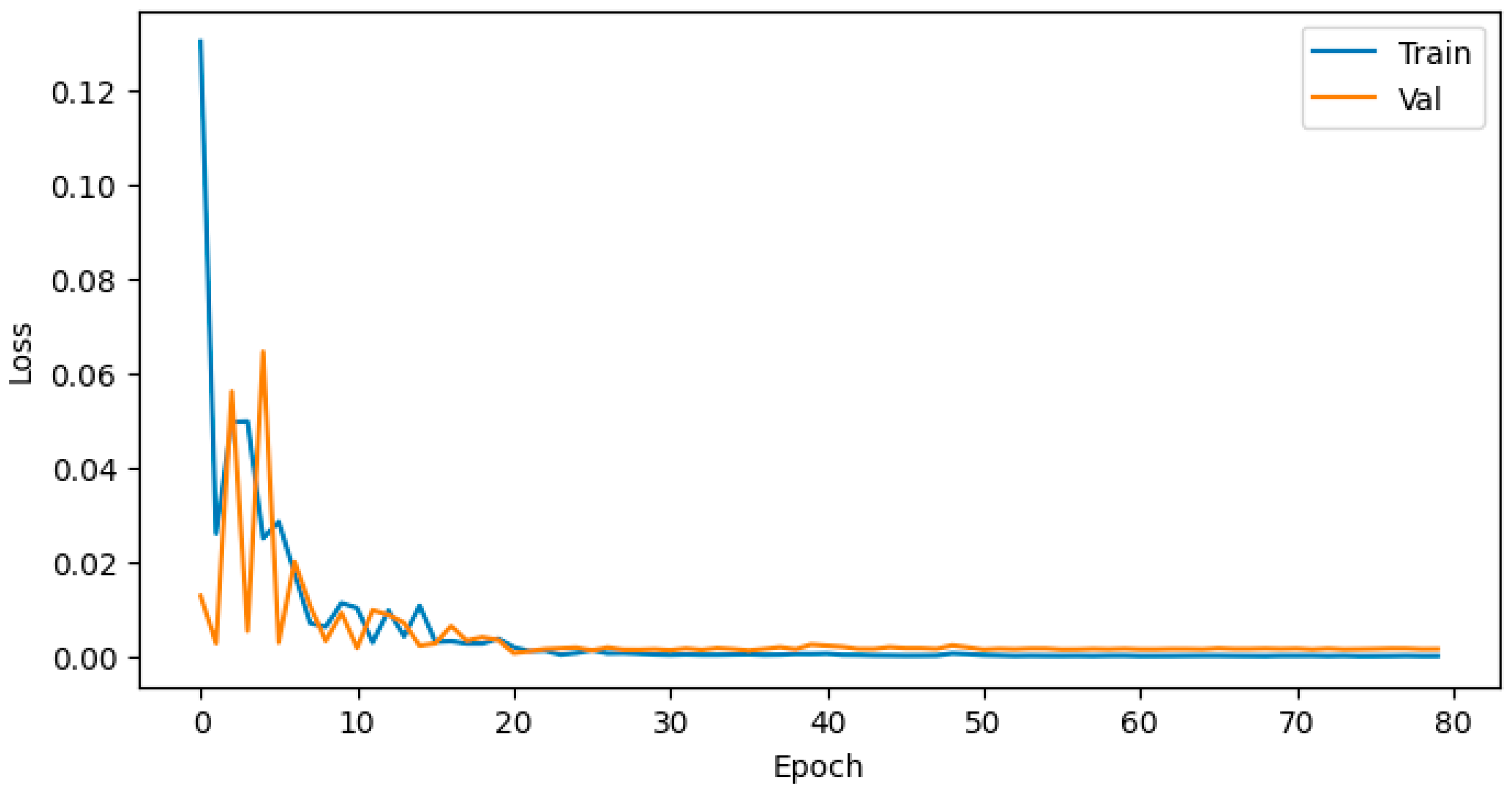
Figure 16 shows the training and validation MAE loss for the severity model with S = 0.5 m for Seed 10. Many trials were performed to stop the analysis at epoch 20, but the test results and other metrics improved beyond epoch 70, reaching 80 epochs. The other training cases, corresponding to different values of “S” and seed numbers, have a similar training curve.

Figure 17 illustrates the training data and validation data loss calculated using the smooth L1 loss function for location over epochs regarding the location model with sample S = 1 m for seed 20. The loss value decreased by increasing epochs and remained constant until 150 epochs were completed. Starting from epoch 110, the training and validation losses were close to each other. The remaining 14 models, with different S values and seeds, have similar curve shapes and behaviors.

4.2. Test Metrics

To evaluate model performance, a separate test dataset, completely different from the training and validation data, called test data, is used. This dataset indicates whether the model generalizes better or worse than before. Different metrics are used to state the condition of the model, such as the R² score and the MAE. Since the location model has a more complicated architecture than severity model, additional metrics are performed only on the location model to enable deeper evaluation, such as the 90th percentile error (P90), 95th percentile error (P95) [82], and the percentage of data predictions within a fixed tolerance ($\pm$0.5 m error).

The R² score is a statistical metric that determines how well a regression model fits the observed data [83]. It shows the percentage of the dependent variable’s (target) variance that can be accounted for by the model’s independent variables (features). The R² is performed on the test data as follows:

$${\mathrm{R}}^2=1-{\displaystyle \frac{\sum {({\mathrm{y}}_{\mathrm{t}\mathrm{e}\mathrm{s}\mathrm{t}}-{\widehat{\mathrm{y}}}_{\mathrm{t}\mathrm{e}\mathrm{s}\mathrm{t}})}^2}{\sum {({\mathrm{y}}_{\mathrm{t}\mathrm{e}\mathrm{s}\mathrm{t}}-{\overline{\mathrm{y}}}_{\mathrm{t}\mathrm{e}\mathrm{s}\mathrm{t}})}^2}}$$

(13)

where ${\mathrm{y}}_{\mathrm{t}\mathrm{e}\mathrm{s}\mathrm{t}}$ is the true target value, ${\widehat{\mathrm{y}}}_{\mathrm{t}\mathrm{e}\mathrm{s}\mathrm{t}}$ is the predicted value from the model, and ${\overline{\mathrm{y}}}_{\mathrm{t}\mathrm{e}\mathrm{s}\mathrm{t}}$ is the mean of the test target values.

Figure 18a illustrates the average R² among seeds using different S values for the severity model. The error bars refer to the SD among the three used seeds. The model with S = 0.1 m has the highest score. Damage severity is mainly based on the TLA values among the cases; therefore, increasing the number of sensors at S = 0.1 m provides sufficient information, allowing the model to be more generalized for damage severity determination with minimum errors across different seeds. The same case is happening while dealing with MAE in Figure 18b, where increasing the number of sensors results in lower errors. However, practical considerations should be taken, as UAVs require at least 0.1 m or greater spacing to avoid collisions.

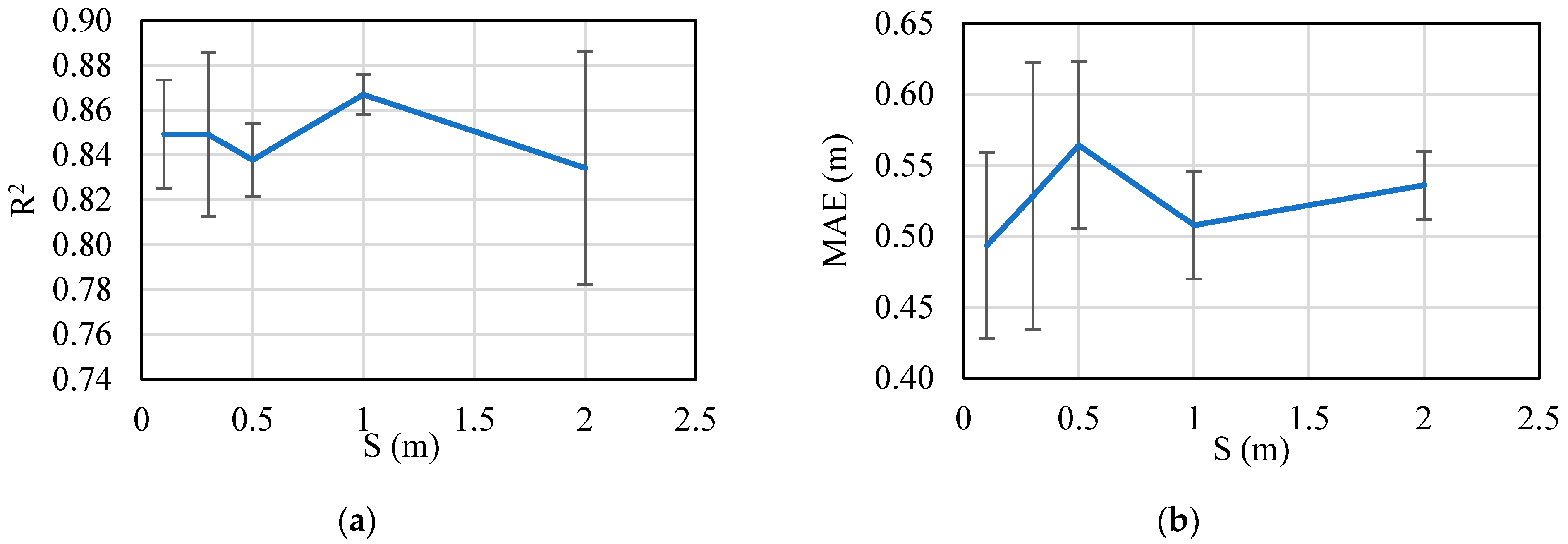
Figure 19a shows the average R² values for different S values regarding the location model. It is noticed that the case with S = 1.0 m has the highest R² score among the cases with minimum SD. This means that a balanced number of sensors, between the maximum for S = 0.1 m and minimum for S = 2 m, yield better training. This is attributed to reducing the noise that could be found from the maximum number of sensors and keeping information unmissed, like the case of S = 2.0 m. Figure 19b shows the corresponding MAE results on the test data for the same model, where S = 1.0 m has lower errors and a balanced SD compared to other cases due to the same balance between the information needed and noise reduction.

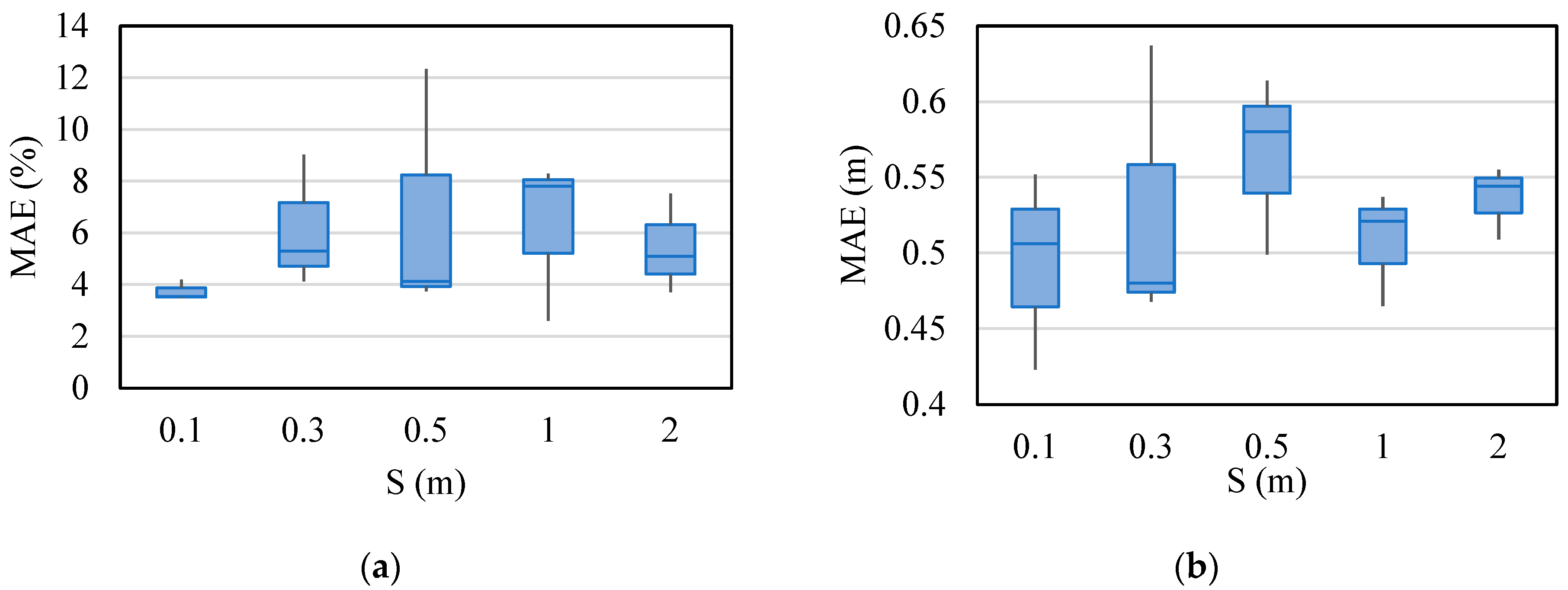
Figure 20a shows the MAE box plot for the test data regarding the severity model. It is obvious that S = 0.1 m is the best performance due to lower errors and narrower ranges while maintaining practicality with respect to UAV dimensions. Figure 20b shows the MAE box plot regarding the location model. Although S = 2.0 m has the smallest range between the maximum and minimum MAE values, the values of S = 2.0 m are still higher than S = 1.0 m regarding maximum, minimum, and quartile values, due to the lack of information using a smaller number of sensors. The values at S = 0.1 m and S = 0.3 m have a higher range of error than S = 1.0 m, because of the presence of noise when using a larger number of sensors. Errors and quartile values are increased at S = 0.5 m and then reduced significantly at S = 1.0 m, due to the balance between the noise and the information needed.

Table 2. Average performance metrics for the location model across different spacings (S).

S (m)	P90 (m)	P95 (m)	% ≤ 0.5 m
0.1	1.84 ± 0.09	2.16 ± 0.15	80.5 ± 4.8
0.3	1.96 ± 0.25	2.15 ± 0.25	75.0 ± 8.3
0.5	1.93 ± 0.08	2.21 ± 0.13	69.4 ± 12.7
1	1.64 ± 0.22	1.98 ± 0.08	77.8 ± 4.8
2	2.00 ± 0.43	2.22 ± 0.49	75.0 ± 14.4

shows the average values of metrics P90, P95, and the percentage of predictions that are lower than tolerance 0.5 m regarding the location model, in addition to the SD in each case among seeds. The P90 and P95 error bounds reveal that the model achieves the most consistent damage localization at S = 1.0 m, while S = 2.0 m misses key response variations. In contrast, dense spacings at S $\le$ 0.3 m introduce excessive noise. Accordingly, the 1 m spacing provides an optimal balance with the lowest P95 (1.98 ± 0.08 m) and maintains over 77% of predictions within ±0.5 m, indicating reliable field precision within 5% of the bridge span.

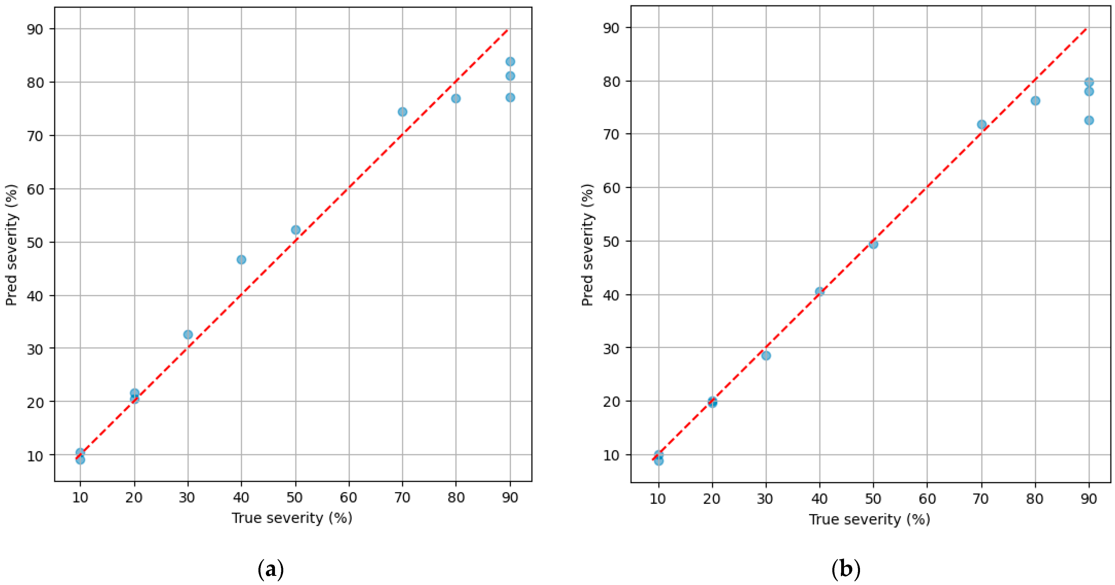
Figure 21a shows the 45° agreement line between the predictions and the true values of the severity model, with the best performance at S = 0.1 m. Figure 21b shows the same data for a case using S = 0.5 m. All the models predicted most of the test cases to be true, as shown in the figure. However, extreme severity such as 90% has a slight deviation from the true values due to the noise that happens in the data near the highest damage severity values.

Figure 22a shows the 45° agreement line between the predictions and the true values of the location model, with the best performance at S = 1.0 m. Figure 22b shows the same data for the worst case for S = 2.0 m. Regardless of the performance, most of the test data predicted are the same as the true values in all cases, as shown in both figures, with the average R² score having a narrow range between 0.83 and 0.88 for all the used models.

4.3. Damage Prediction

The main purpose of this paper is to detect the damage location and severity from field data, as the predefined case from the UAV deployment, as shown in the proposed framework. The ground truth case, which has damage at location 5.0 m with severity 15%, is passed through all models regarding different seeds.

Table 3. Average damage prediction values for WaveNet models.

S (m)	Predicted Location (m)	Predicted Severity (%)
0.1	5.233 ± 0.138	14.00 ± 0.97
0.3	5.037 ± 0.061	13.58 ± 0.64
0.5	4.983 ± 0.163	14.57 ± 0.27
1	5.092 ± 0.054	14.02 ± 0.39
2	5.046 ± 0.130	14.40 ± 0.69

shows the average prediction results of this assumed field case using all S variables with their SD among seeds. The results show that regardless of the model type, the prediction made is close to the target ones for both models. However, the location model achieved its highest accuracy at S = 1.0 m (bias = 0.09 m, SD ± 0.05 m), which agrees with the training and test results.

For the severity model, although S = 0.1 had the best performance with the highest R² and smallest MAE, its larger variability across seeds (SD ± 0.97%) reflects the sensitivity to high noise from using the highest number of sensors. The nearest model average was at S = 0.5 m with greater stability (SD ± 0.27%). This means that moderate densification allows the network to generalize more consistently.

5. Summary and Discussion of Results

A DL pretrained WaveNet framework is implemented to train acceleration data from a 10 m span bridge and predict the damage of an unknown case for the same bridge.

For the severity model, the model achieves its highest coefficient at S = 0.1 (Figure 18a). This indicates that dense sampling provides rich amplitude information from the TLA signals that directly governs severity. This trend is mirrored in MAE (see Figure 18b), which means that finer spacing generally yields lower errors. Nevertheless, the seed-to-seed variability grows at the densest layout, reflecting sensitivity to high-frequency noise and correlated inputs when sensors are very close. The MAE shown in Figure 20a shows that S = 0.1 m attains the lowest median error and tightest interquartile range, explaining that a dense layout is well suited for severity estimation. However, practical considerations for UAV deployment should be taken into account because minimum spacing such as S = 0.1–0.3 m is already near the collision distance of the UAVs because of their dimensions. In orchestrated UAV inspection, the spacing S refers to the center-to-center distance between UAV-mounted sensors in each configuration. Compact UAVs are suitable for carrying sensors, such as the Parrot Anafi Ai or DJI Air 3, have total spans of approximately 0.33–0.4 m, including propellers [84,85]. Considering UAV dimensions and the minimum safe clearance required for stable operation, S = 0.1–0.3 m would provide insufficient physical distance between UAVs. Maintaining S ≥ 0.5 m ensures adequate clearance for safe maneuvering and reliable data while preserving dense spatial coverage. This quantitative reasoning supports the choice of S = 0.5 m as a practical and safe configuration for field deployment. Importantly, S = 0.5 m emerges as a robust alternative with lower average accuracy.

For the location model, the training results revealed a clear tradeoff between sensor spacing and model performance that can be interpreted through both structural and machine learning perspectives. When the spacing is coarse (e.g., S = 2 m), the number of available sensors is relatively small. This reduces noise input, which makes the training easier but eliminating important acceleration features. As a result, the model tends to underfit with a lower R² score (see Figure 19a) and higher error metrics for the test data (Figure 19b). Conversely, with very dense spacing (e.g., S = 0.1 m), the model has access to many sensors and provides rich dynamic information, but these features introduce redundancy and amplify noise, leading to lower predictive accuracy. In contrast, intermediate spacing (e.g., S = 1 m) provides a balanced configuration (Figure 20b), as the model retains enough structural information to capture localized bridge responses while avoiding excessive noise. This balance test results in the best overall performance, with higher R² and reduced error measures.

Moreover, distribution-based metrics are applied on the test data to provide a more accurate assessment of the location model as provided in Table 2, such as P90, P95, and the percentage of predictions within a fixed tolerance of 0.5 m. Lower P90 and P95 values, which have average values of 16% and 1%, respectively, of the bridge span for the intermediate spacing case (S = 1 m), indicate that extreme errors are kept under control for SHM safety applications where outliers can lead to false detections. Similarly, reporting the percentage of predictions with tolerance ± 0.5 m quantifies practical accuracy relative to the bridge span. For the bridge span of 10 m studied, this tolerance corresponds only to 5% of the total length, illustrating that predictions are accurate and meaningful. Large values are detected for this percentage, with an approximate range of 70% to 80% for all cases and an average of 77.8% for the S = 1.0 m case with ± 4.8% SD. Together, these indicators reinforce the observation that intermediate sensor spacing (e.g., S = 1 m) not only improves average accuracy but also reduces the likelihood of large prediction errors, making it a more reliable choice for real-world deployment.

To assess end-to-end utility, the fixed field scenario (damage at 5.0 m, 15% severity) was evaluated across all models and seeds. Table 3 reports the mean ± SD predictions versus sensor spacing.

From a severity perspective, the pattern differs, as case S = 0.1 m achieves the highest accuracy in the training stage because severity is driven by the amplitude scaling of TLA signals. For the damage severity prediction, the most stable and precise case was S = 0.5 m (14.57% ± 0.27%), which reduces sensitivity to high-frequency noise while maintaining sufficient spatial information. Damage localization is most accurate and stable for the intermediate case S = 1.0 m (bias = 0.09 m, SD ± 0.05 m). This case concludes an optimal balance between information richness (capturing local vibration gradients near the defect) and noise existence (avoiding redundancy from overly dense arrays). At coarser spacing (e.g., S = 2.0 m), the predicted damage location has the same SD value as the densest layout case (e.g., S = 0.1 m).

If a single spacing is required for both tasks (localization and severity), S = 1.0 offers excellent localization with near-target severity (14.02% ± 0.39%). Moreover, it maintains practical deployment by preventing UAV collisions with each other, as previously discussed. Ultimately, these results demonstrate that optimal spacing is task dependent: location favors balanced intermediate density, whereas severity favors dense to moderately dense layouts. Both converge to accurate field predictions under realistic sensing constraints.

While the present study demonstrates the promising predictive performance of the pretrained WaveNet framework, it is based on a focused FE dataset representing a single bridge typology and systematically varied damage cases (82 cases). The controlled design allows precise evaluation of the model’s sensitivity to sensor spacing and noise while maintaining interpretability of results. However, extending the dataset by using different bridge geometries, spans, and excitation scenarios will further test generalization under real-world noise conditions. Future research will incorporate cross-bridge validation and randomization for loading conditions to quantify model robustness. These expansions will build on the current foundation to demonstrate the scalability of the proposed framework for broader SHM applications.

6. Conclusions and Recommendations

6.1. Conclusions

This paper introduced a WaveNet-based DL framework for detecting local bridge damage using the orchestrated UAV sensing concept. Two models were developed for damage location and severity prediction under different sensor spacings “S”. Training, testing, and prediction were carried out for both models. Accordingly, the conclusions are listed below as follows:

• The severity model performed best with dense to moderately dense UAV layouts. While S = 0.1 m achieved the highest accuracy during training, the practical optimum S = 0.5 m yields near-target means and the lowest SD among seeds. This balance between information richness and noise control ensures strong robustness during both training and testing.
• The location model is evaluated with the highest accuracy at S = 1.0 m, including the highest R² and lowest MAE, P90, and P95. This spacing provides enough spatial resolution to capture local gradients without amplifying noise or redundancy.
• Coarse spacing (S = 2.0 m) for location model underfits and misses local features, while denser spacings (S $\le$ 0.3 m) can overfit or become noise sensitive. Therefore, the intermediate S = 1.0 m minimizes both bias and SD for localization.

6.2. Recommendations

• Various bridge dimensions and conditions could be used through the WaveNet framework, depending on the availability of the bridge dataset.
• A comparison may be conducted between the proposed WaveNet Framework and other DL models (e.g., CNN, LSTM, GRU) using the same dataset to quantitatively evaluate relative accuracy, convergence speed, and stability.

References

1. Aktan, A.; Catbas, F.N.; Grimmelsman, K.; Tsikos, C. Issues in infrastructure health monitoring for management. J. Eng. Mech. 2000, 126, 711–724. [Google Scholar] [CrossRef]
2. Phares, B.M.; Washer, G.A.; Rolander, D.D.; Graybeal, B.A.; Moore, M. Routine highway bridge inspection condition documentation accuracy and reliability. J. Bridge Eng. 2004, 9, 403–413. [Google Scholar] [CrossRef]
3. Mitra, M.; Gopalakrishnan, S. Guided wave based structural health monitoring: A review. Smart Mater. Struct. 2016, 25, 053001. [Google Scholar] [CrossRef]
4. Cawley, P. Structural health monitoring: Closing the gap between research and industrial deployment. Struct. Health Monit. 2018, 17, 1225–1244. [Google Scholar] [CrossRef]
5. He, Z.; Li, W.; Salehi, H.; Zhang, H.; Zhou, H.; Jiao, P. Integrated structural health monitoring in bridge engineering. Autom. Constr. 2022, 136, 104168. [Google Scholar] [CrossRef]
6. Yu, X.; Fu, Y.; Li, J.; Mao, J.; Hoang, T.; Wang, H. Recent advances in wireless sensor networks for structural health monitoring of civil infrastructure. J. Infrastruct. Intell. Resil. 2024, 3, 100066. [Google Scholar] [CrossRef]
7. Sonbul, O.S.; Rashid, M. Towards the structural health monitoring of bridges using wireless sensor networks: A systematic study. Sensors 2023, 23, 8468. [Google Scholar] [CrossRef]
8. Zelenika, S.; Hadas, Z.; Bader, S.; Becker, T.; Gljušćić, P.; Hlinka, J.; Janak, L.; Kamenar, E.; Ksica, F.; Kyratsi, T. Energy harvesting technologies for structural health monitoring of airplane components—A review. Sensors 2020, 20, 6685. [Google Scholar] [CrossRef]
9. Spencer Jr, B.; Ruiz-Sandoval, M.E.; Kurata, N. Smart sensing technology: Opportunities and challenges. Struct. Control Health Monit. 2004, 11, 349–368. [Google Scholar] [CrossRef]
10. Entezami, A.; Sarmadi, H.; Behkamal, B.; Mariani, S. Big data analytics and structural health monitoring: A statistical pattern recognition-based approach. Sensors 2020, 20, 2328. [Google Scholar] [CrossRef]
11. Armijo, A.; Zamora-Sánchez, D. Integration of Railway Bridge Structural Health Monitoring into the Internet of Things with a Digital Twin: A Case Study. Sensors 2024, 24, 2115. [Google Scholar] [CrossRef]
12. Cha, Y.-J.; Ali, R.; Lewis, J.; Büyüköztürk, O. Deep learning-based structural health monitoring. Autom. Constr. 2024, 161, 105328. [Google Scholar] [CrossRef]
13. Jia, J.; Li, Y. Deep learning for structural health monitoring: Data, algorithms, applications, challenges, and trends. Sensors 2023, 23, 8824. [Google Scholar] [CrossRef] [PubMed]
14. Elman, J.L. Finding structure in time. Cogn. Sci. 1990, 14, 179–211. [Google Scholar] [CrossRef]
15. Hochreiter, S.; Schmidhuber, J. Long short-term memory. Neural Comput. 1997, 9, 1735–1780. [Google Scholar] [CrossRef]
16. Cho, K.; Van Merriënboer, B.; Gulcehre, C.; Bahdanau, D.; Bougares, F.; Schwenk, H.; Bengio, Y. Learning phrase representations using RNN encoder-decoder for statistical machine translation. arXiv 2014, arXiv:1406.1078. [Google Scholar] [CrossRef]
17. Chung, J.; Gulcehre, C.; Cho, K.; Bengio, Y. Empirical evaluation of gated recurrent neural networks on sequence modeling. arXiv 2014, arXiv:1412.3555. [Google Scholar] [CrossRef]
18. Kiranyaz, S.; Avci, O.; Abdeljaber, O.; Ince, T.; Gabbouj, M.; Inman, D.J. 1D convolutional neural networks and applications: A survey. Mech. Syst. Signal Process. 2021, 151, 107398. [Google Scholar] [CrossRef]
19. Ismail Fawaz, H.; Forestier, G.; Weber, J.; Idoumghar, L.; Muller, P.-A. Deep learning for time series classification: A review. Data Min. Knowl. Discov. 2019, 33, 917–963. [Google Scholar] [CrossRef]
20. LeCun, Y.; Bengio, Y. Convolutional networks for images, speech, and time series. In The Handbook of Brain Theory and Neural Networks; HAL Open Science: Lyon, France, 1998. [Google Scholar]
21. Zhang, G.-Q.; Wang, B.; Li, J.; Xu, Y.-L. The application of deep learning in bridge health monitoring: A literature review. Adv. Bridge Eng. 2022, 3, 22. [Google Scholar] [CrossRef]
22. Floreano, D.; Wood, R.J. Science, technology and the future of small autonomous drones. Nature 2015, 521, 460–466. [Google Scholar] [CrossRef] [PubMed]
23. Sreenath, S.; Malik, H.; Husnu, N.; Kalaichelavan, K. Assessment and use of unmanned aerial vehicle for civil structural health monitoring. Procedia Comput. Sci. 2020, 170, 656–663. [Google Scholar] [CrossRef]
24. Tan, C.; Elhattab, A.; Uddin, N. Wavelet-entropy approach for detection of bridge damages using direct and indirect bridge records. J. Infrastruct. Syst. 2020, 26, 04020037. [Google Scholar] [CrossRef]
25. Elhattab, A.; Uddin, N.; OBrien, E. Drive-by bridge damage monitoring using Bridge Displacement Profile Difference. J. Civ. Struct. Health Monit. 2016, 6, 839–850. [Google Scholar] [CrossRef]
26. Fan, W.; Qiao, P. Vibration-based damage identification methods: A review and comparative study. Struct. Health Monit. 2011, 10, 83–111. [Google Scholar] [CrossRef]
27. Tan, C.; Zhao, H.; OBrien, E.J.; Uddin, N.; Fitzgerald, P.C.; McGetrick, P.J.; Kim, C.-W. Extracting mode shapes from drive-by measurements to detect global and local damage in bridges. Struct. Infrastruct. Eng. 2021, 17, 1582–1596. [Google Scholar] [CrossRef]
28. Kariyawasam, K.D.; Middleton, C.R.; Madabhushi, G.; Haigh, S.K.; Talbot, J.P. Assessment of bridge natural frequency as an indicator of scour using centrifuge modelling. J. Civ. Struct. Health Monit. 2020, 10, 861–881. [Google Scholar] [CrossRef]
29. Van Den Oord, A.; Dieleman, S.; Zen, H.; Simonyan, K.; Vinyals, O.; Graves, A.; Kalchbrenner, N.; Senior, A.; Kavukcuoglu, K. Wavenet: A generative model for raw audio. arXiv 2016, arXiv:1609.03499. [Google Scholar] [CrossRef]
30. Mariani, S.; Rendu, Q.; Urbani, M.; Sbarufatti, C. Causal dilated convolutional neural networks for automatic inspection of ultrasonic signals in non-destructive evaluation and structural health monitoring. Mech. Syst. Signal Process. 2021, 157, 107748. [Google Scholar] [CrossRef]
31. Oord, A.; Li, Y.; Babuschkin, I.; Simonyan, K.; Vinyals, O.; Kavukcuoglu, K.; Driessche, G.; Lockhart, E.; Cobo, L.; Stimberg, F. Parallel wavenet: Fast high-fidelity speech synthesis. In Proceedings of the International Conference on Machine Learning, Stockholm, Sweden, 10–15 July 2018; pp. 3918–3926. [Google Scholar]
32. Engel, J.; Resnick, C.; Roberts, A.; Dieleman, S.; Norouzi, M.; Eck, D.; Simonyan, K. Neural audio synthesis of musical notes with wavenet autoencoders. In Proceedings of the International Conference on Machine Learning, Sydney, Australia, 6–11 August 2017; pp. 1068–1077. [Google Scholar]
33. Rethage, D.; Pons, J.; Serra, X. A wavenet for speech denoising. In Proceedings of the 2018 IEEE International Conference on Acoustics, Speech and Signal Processing (ICASSP), Calgary, AB, Canada, 15–20 April 2018; pp. 5069–5073. [Google Scholar]
34. Pankka, H.; Lehtinen, J.; Ilmoniemi, R.J.; Roine, T. Forecasting EEG time series with WaveNet. bioRxiv 2024. [Google Scholar] [CrossRef]
35. Lv, T.; Tao, A.; Zhang, Z.; Qin, S.; Wang, G. Significant wave height prediction based on the local-EMD-WaveNet model. Ocean Eng. 2023, 287, 115900. [Google Scholar] [CrossRef]
36. Oh, S.L.; Jahmunah, V.; Ooi, C.P.; Tan, R.-S.; Ciaccio, E.J.; Yamakawa, T.; Tanabe, M.; Kobayashi, M.; Acharya, U.R. Classification of heart sound signals using a novel deep WaveNet model. Comput. Methods Programs Biomed. 2020, 196, 105604. [Google Scholar] [CrossRef] [PubMed]
37. Dorado Rueda, F.; Durán Suárez, J.; del Real Torres, A. Short-term load forecasting using encoder-decoder wavenet: Application to the french grid. Energies 2021, 14, 2524. [Google Scholar] [CrossRef]
38. Ning, C.; Xie, Y.; Sun, L. LSTM, WaveNet, and 2D CNN for nonlinear time history prediction of seismic responses. Eng. Struct. 2023, 286, 116083. [Google Scholar] [CrossRef]
39. Mariani, S.; Kalantari, A.; Kromanis, R.; Marzani, A. Data-driven modeling of long temperature time-series to capture the thermal behavior of bridges for SHM purposes. Mech. Syst. Signal Process. 2024, 206, 110934. [Google Scholar] [CrossRef]
40. Psathas, A.P.; Iliadis, L.; Achillopoulou, D.V.; Papaleonidas, A.; Stamataki, N.K.; Bountas, D.; Dokas, I.M. Autoregressive deep learning models for bridge strain prediction. In Proceedings of the International Conference on Engineering Applications of Neural Networks, Chersonissos, Crete, Greece, 17–20 June 2022; pp. 150–164. [Google Scholar]
41. Dabbous, A.; Berta, R.; Fresta, M.; Ballout, H.; Lazzaroni, L.; Bellotti, F. Bringing Intelligence to the Edge for Structural Health Monitoring. The Case Study of the Z24 Bridge. IEEE Open J. Ind. Electron. Soc. 2024, 5, 781–794. [Google Scholar] [CrossRef]
42. Gaebler, K.O.; Shield, C.K.; Linderman, L.E. Feasibility of Vibration-Based Long-Term Bridge Monitoring Using the I-35W St. Anthony Falls Bridge; Minnesota Department of Transportation: Saint Paul, MN, USA, 2017. [Google Scholar]
43. Yang, Y.; Lin, C.; Yau, J. Extracting bridge frequencies from the dynamic response of a passing vehicle. J. Sound Vib. 2004, 272, 471–493. [Google Scholar] [CrossRef]
44. Yang, Y.; Chang, K. Extracting the bridge frequencies indirectly from a passing vehicle: Parametric study. Eng. Struct. 2009, 31, 2448–2459. [Google Scholar] [CrossRef]
45. Keenahan, J.; McGetrick, P.; O’Brien, E.J.; Gonzalez, A. Using instrumented vehicles to detect damage in bridges. In Proceedings of the 15th International Conference on Experimental Mechanics, Porto, Portugal, 22–27 July 2012. [Google Scholar]
46. Eshkevari, S.S.; Matarazzo, T.J.; Pakzad, S.N. Bridge modal identification using acceleration measurements within moving vehicles. Mech. Syst. Signal Process. 2020, 141, 106733. [Google Scholar] [CrossRef]
47. Neubauer, K.; Bullard, E.; Blunt, R. Collection of Data with Unmanned Aerial Systems (UAS) for Bridge Inspection and Construction Inspection; United States Department of Transportation, Federal Highway Administration: Washington, DC, USA, 2021.
48. Khan, M.A.; McCrum, D.P.; OBrien, E.J.; Bowe, C.; Hester, D.; McGetrick, P.J.; O’Higgins, C.; Casero, M.; Pakrashi, V. Re-deployable sensors for modal estimates of bridges and detection of damage-induced changes in boundary conditions. Struct. Infrastruct. Eng. 2022, 18, 1177–1191. [Google Scholar] [CrossRef]
49. Malekjafarian, A.; OBrien, E.J. Identification of bridge mode shapes using short time frequency domain decomposition of the responses measured in a passing vehicle. Eng. Struct. 2014, 81, 386–397. [Google Scholar] [CrossRef]
50. Liu, H.; Tian, H.; Wang, D.; Yuan, T.; Zhang, J.; Liu, G.; Li, X.; Chen, X.; Wang, C.; Cai, S. Electrically active smart adhesive for a perching-and-takeoff robot. Sci. Adv. 2023, 9, eadj3133. [Google Scholar] [CrossRef]
51. Lussier Desbiens, A.; Cutkosky, M.R. Landing and perching on vertical surfaces with microspines for small unmanned air vehicles. J. Intell. Robot. Syst. 2010, 57, 313–327. [Google Scholar] [CrossRef]
52. Harris, C.R.; Millman, K.J.; Van Der Walt, S.J.; Gommers, R.; Virtanen, P.; Cournapeau, D.; Wieser, E.; Taylor, J.; Berg, S.; Smith, N.J. Array programming with NumPy. Nature 2020, 585, 357–362. [Google Scholar] [CrossRef] [PubMed]
53. McKinney, W. Data structures for statistical computing in Python. Scipy 2010, 445, 51–56. [Google Scholar]
54. Paszke, A.; Gross, S.; Massa, F.; Lerer, A.; Bradbury, J.; Chanan, G.; Killeen, T.; Lin, Z.; Gimelshein, N.; Antiga, L. Pytorch: An imperative style, high-performance deep learning library. In Proceedings of the Advances in Neural Information Processing Systems, Vancouver, BC, Canada, 8–14 December 2019; Volume 32. [Google Scholar]
55. Hunter, J.D. Matplotlib: A 2D graphics environment. Comput. Sci. Eng. 2007, 9, 90–95. [Google Scholar] [CrossRef]
56. Abdellatef, A.I.M. Integrated Structural Health Monitoring Techniques Using Drone Sensors. Ph.D. Thesis, The University of Alabama at Birmingham, Birmingham, AL, USA, 2022. [Google Scholar]
57. Christides, S.; Barr, A. One-dimensional theory of cracked Bernoulli-Euler beams. Int. J. Mech. Sci. 1984, 26, 639–648. [Google Scholar] [CrossRef]
58. Shen, M.-H.; Pierre, C. Natural modes of Bernoulli-Euler beams with symmetric cracks. J. Sound Vib. 1990, 138, 115–134. [Google Scholar] [CrossRef]
59. Shen, M.-H.; Pierre, C. Free vibrations of beams with a single-edge crack. J. Sound Vib. 1994, 170, 237–259. [Google Scholar] [CrossRef]
60. Weng, J.; Lee, C.K.; Tan, K.H.; Lim, N.S. Damage assessment for reinforced concrete frames subject to progressive collapse. Eng. Struct. 2017, 149, 147–160. [Google Scholar] [CrossRef]
61. Avci, O.; Abdeljaber, O.; Kiranyaz, S.; Hussein, M.; Gabbouj, M.; Inman, D.J. A review of vibration-based damage detection in civil structures: From traditional methods to Machine Learning and Deep Learning applications. Mech. Syst. Signal Process. 2021, 147, 107077. [Google Scholar] [CrossRef]
62. Sinha, J.K.; Friswell, M.; Edwards, S. Simplified models for the location of cracks in beam structures using measured vibration data. J. Sound Vib. 2002, 251, 13–38. [Google Scholar] [CrossRef]
63. Zhu, X.; Law, S. Wavelet-based crack identification of bridge beam from operational deflection time history. Int. J. Solids Struct. 2006, 43, 2299–2317. [Google Scholar] [CrossRef]
64. Zhang, Y.; Pintea, S.L.; Van Gemert, J.C. Video acceleration magnification. In Proceedings of the IEEE Conference on Computer Vision and Pattern Recognition, Honolulu, HI, USA, 21–26 July 2017; pp. 529–537. [Google Scholar]
65. Voth, G.A.; La Porta, A.; Crawford, A.M.; Alexander, J.; Bodenschatz, E. Measurement of particle accelerations in fully developed turbulence. J. Fluid Mech. 2002, 469, 121–160. [Google Scholar] [CrossRef]
66. Goodfellow, I.; Bengio, Y.; Courville, A.; Bengio, Y. Deep Learning; MIT Press: Cambridge, MA, USA, 2016; Volume 1. [Google Scholar]
67. Zhao, C.; Wang, Y.; Zhang, X.; Chen, S.; Wu, C.; Teo, K.L. UAV dispatch planning for a wireless rechargeable sensor network for bridge monitoring. IEEE Trans. Sustain. Comput. 2022, 8, 293–309. [Google Scholar] [CrossRef]
68. Salimans, T.; Kingma, D.P. Weight normalization: A simple reparameterization to accelerate training of deep neural networks. In Proceedings of the Advances in Neural Information Processing Systems, Barcelona, Spain, 5–10 December 2016; Volume 29. [Google Scholar]
69. Wu, Y.; He, K. Group normalization. In Proceedings of the European Conference on Computer Vision (ECCV), Munich, Germany, 8–14 September 2018; pp. 3–19. [Google Scholar]
70. Srivastava, N.; Hinton, G.; Krizhevsky, A.; Sutskever, I.; Salakhutdinov, R. Dropout: A simple way to prevent neural networks from overfitting. J. Mach. Learn. Res. 2014, 15, 1929–1958. [Google Scholar]
71. Ghiasi, G.; Lin, T.-Y.; Le, Q.V. Dropblock: A regularization method for convolutional networks. In Proceedings of the Advances in Neural Information Processing Systems, Montréal, QC, Canada, 3–8 December 2018; Volume 31. [Google Scholar]
72. Kim, B.J.; Choi, H.; Jang, H.; Lee, D.; Kim, S.W. How to use dropout correctly on residual networks with batch normalization. In Proceedings of the Uncertainty in Artificial Intelligence, Pittsburgh, PA, USA, 31 July–4 August 2023; pp. 1058–1067. [Google Scholar]
73. Glorot, X.; Bordes, A.; Bengio, Y. Deep sparse rectifier neural networks. In Proceedings of the Fourteenth International Conference on Artificial Intelligence and Statistics, Fort Lauderdale, FL, USA, 11–13 April 2011; pp. 315–323. [Google Scholar]
74. Bishop, C.M.; Nasrabadi, N.M. Pattern Recognition and Machine Learning; Springer: New York, NY, USA, 2006; Volume 4. [Google Scholar]
75. Huber, P.J. Robust estimation of a location parameter. In Breakthroughs in Statistics: Methodology and Distribution; Springer: New York, NY, USA, 1992; pp. 492–518. [Google Scholar]
76. Girshick, R. Fast r-cnn. In Proceedings of the IEEE International Conference on Computer Vision, Santiago, Chile, 7–13 December 2015; pp. 1440–1448. [Google Scholar]
77. Ainsworth, M.; Shin, Y. Plateau phenomenon in gradient descent training of RELU networks: Explanation, quantification, and avoidance. SIAM J. Sci. Comput. 2021, 43, A3438–A3468. [Google Scholar] [CrossRef]
78. Loshchilov, I.; Hutter, F. Sgdr: Stochastic gradient descent with warm restarts. arXiv 2016, arXiv:1608.03983. [Google Scholar]
79. Liaw, R.; Liang, E.; Nishihara, R.; Moritz, P.; Gonzalez, J.E.; Stoica, I. Tune: A research platform for distributed model selection and training. arXiv 2018, arXiv:1807.05118. [Google Scholar] [CrossRef]
80. Park, D.S.; Chan, W.; Zhang, Y.; Chiu, C.-C.; Zoph, B.; Cubuk, E.D.; Le, Q.V. Specaugment: A simple data augmentation method for automatic speech recognition. arXiv 2019, arXiv:1904.08779. [Google Scholar] [CrossRef]
81. Izmailov, P.; Podoprikhin, D.; Garipov, T.; Vetrov, D.; Wilson, A.G. Averaging weights leads to wider optima and better generalization. arXiv 2018, arXiv:1803.05407. [Google Scholar]
82. Falcetelli, F.; Yue, N.; Di Sante, R.; Zarouchas, D. Probability of detection, localization, and sizing: The evolution of reliability metrics in Structural Health Monitoring. Struct. Health Monit. 2022, 21, 2990–3017. [Google Scholar] [CrossRef]
83. Fisher, R.A. Statistical Methods for Research Workers; Oliver and Boyd: Edinburgh, UK, 1928. [Google Scholar]
84. Parrot. Anafi Ai Technical Specifications. Available online: https://www.parrot.com/en/drones/anafi-ai (accessed on 3 November 2025).
85. DJI. Air 3 Product Specifications. Available online: https://www.dji.com/air-3/specs (accessed on 3 November 2025).
Figure 1. Similarity between acceleration data and sound data: (a) Acceleration time data; (b) Sound wave data. The dash line represents the zero reference level.
Applsci 15 12228 g001
Figure 2. Damage detection using a WaveNet model.
Applsci 15 12228 g002
Figure 3. Orchestrated UAV deployment [48].
Applsci 15 12228 g003
Figure 4. Bridge structural system.
Applsci 15 12228 g004
Figure 5. UAV setup: (a) Perching mechanism (b) Sensing application.
Applsci 15 12228 g005
Figure 6. The WaveNet framework steps. Blue boxes indicate processing and modeling steps, while the red box denotes the final output stage.
Applsci 15 12228 g006
Figure 7. Quarter-car model.
Applsci 15 12228 g007
Figure 8. Indication of damage on the bridge.
Applsci 15 12228 g008
Figure 9. Flexural stiffness reduction in the crack location with 50% damage.
Applsci 15 12228 g009
Figure 10. TLA values for a single channel (sensor) after standardization. The dash line represents the zero reference level.
Applsci 15 12228 g010
Figure 11. WaveNet severity model architecture.
Applsci 15 12228 g011
Figure 12. Convolution types: (a) Standard Convolution; (b) Causal Convolution.
Applsci 15 12228 g012
Figure 13. WaveNet dilated causal convolution layers [29].
Applsci 15 12228 g013
Figure 14. WaveNet location model architecture.
Applsci 15 12228 g014
Figure 15. Tune framework interface with two different APIs [79].
Applsci 15 12228 g015
Figure 16. Training and validation loss over epochs for the damage severity model.
Applsci 15 12228 g016
Figure 17. Training and validation loss over epochs for the damage location model.
Applsci 15 12228 g017
Figure 18. Test data results for the severity model: (a) R2 Score; (b) MAE Values.
Applsci 15 12228 g018
Figure 19. Test data results for the location model: (a) R2 Score; (b) MAE Values.
Applsci 15 12228 g019
Figure 20. MAE distribution for WaveNet models under different sensor spacings (S): (a) Severity model; (b) Location model.
Applsci 15 12228 g020
Figure 21. True prediction relationship with the dashed 45° agreement line of the severity model: (a) S = 1.0 m; (b) S = 0.5 m. The blue dots represent the predicted values, while the red dashed line denotes the perfect one-to-one agreement between prediction and ground truth.
Applsci 15 12228 g021
Figure 22. True prediction relationship with the dashed 45° agreement line of the location model: (a) S = 1.0 m; (b) S = 2.0 m. The blue dots represent the predicted values, while the red dashed line denotes the perfect one-to-one agreement between prediction and ground truth.
Applsci 15 12228 g022