Article

Bayesian Optimisation with Dimensionless Groups: A Synergy of Performance and Fundamental Understanding

1
Applied Artificial Intelligence Initiative, Deakin University, 75 Pigdons Road, Waurn Ponds, VIC 3216, Australia
2
School of Engineering, Deakin University, 75 Pigdons Road, Waurn Ponds, VIC 3216, Australia
3
Institute for Frontier Materials, Deakin University, 75 Pigdons Road, Waurn Ponds, VIC 3216, Australia
4
HeiQ Pty Ltd., Geelong, VIC 3220, Australia
*
Author to whom correspondence should be addressed.
These authors contributed equally to this work.
Appl. Sci. 2025, 15(22), 12215; https://doi.org/10.3390/app152212215
Submission received: 14 August 2025 / Revised: 10 November 2025 / Accepted: 14 November 2025 / Published: 18 November 2025
(This article belongs to the Section Computing and Artificial Intelligence)

Abstract

Dimensionless groups quantify the balance among key forces governing a system’s physical behaviour and are foundational in engineering for describing, comparing, and scaling processes. By condensing complex system interactions into single values, they provide a powerful means of abstraction. Yet, their potential to actively guide process optimisation remains largely untapped. This study presents a framework that integrates dimensionless analysis with Bayesian optimisation to enhance both process performance and interpretability. Using this combined approach, we demonstrate that optimisation conducted in the dimensionless space not only accelerates convergence towards optimal process conditions but also reveals the underlying physical balances driving system behaviour. The method thus bridges data-driven optimisation with physically grounded understanding, enabling more efficient and explainable control of complex manufacturing processes.

1. Introduction

Dimensional analysis is well established as being an efficient way to map and compare processes across scales in engineering. It involves identifying a system’s key parameters and combining them into dimensionless entities, known as dimensionless groups, following the Buckingham π theorem. These groups represent balances of forces or other system drivers and are widely used to define regimes of operation. For instance, the Reynolds number—the ratio of inertial to viscous forces in fluid flow—separates laminar and turbulent regimes and is often used in fluid dynamics. Dimensionless numbers enable process scale-up by ensuring that conditions at different scales share identical underlying force balances, thus preserving behaviour and outcomes. They can be viewed as “process equivalents” of colligative properties: by condensing multiple variables into one quantity, they collapse a wealth of information into a single meaningful descriptor. This condensation of information into dimensionless numbers is possible because, in most experimental systems, the variables are related through physical constraints (mathematical relationships among variables) and system-specific conditions (e.g., fixed volume, constant pressure). These correlations render some of the information embedded in the original variables redundant or inconsequential. The Buckingham π theorem filters out such redundancy, retaining the relevant system variability in just a few dimensionless numbers. While useful on their own for scaling processes, combinations of dimensionless numbers are often required to map systems with complex variable interactions, such as multiphase fluid dynamics [1]. However, identifying the most influential dimensionless groups or combinations that lead to deeper system understanding is often difficult and typically requires substantial experimental effort [1]. Dimensionless numbers have been well studied in the literature and are most often used for scaling, system description, or regime identification. Only a few studies have attempted to combine dimensionless groups with machine-learning methods [2,3,4], and these focus mainly on predictive modelling or optimisation guidance rather than revealing the mechanisms that determine system behaviour. Other optimisation strategies have incorporated dimensionless groups only as post-processing tools to generalise outcomes, without embedding them directly into the optimisation loop [5].
Building towards greater insight, Zhu et al. recently demonstrated that dimensionless groups can enhance interpretability and predictive performance in machine-learning models of sonochemical systems [6]. However, their approach remains model centred, with mechanistic insight extracted only post hoc from predictor interpretation. In contrast, the present study embeds dimensionless groups directly within a closed-loop Bayesian optimisation framework applied to a real manufacturing system, allowing physical understanding to emerge within the optimisation process itself rather than after it. This enables the simultaneous refinement of process conditions and governing-mechanism insight during experimentation.
Design of Experiments (DoEs) approaches, and more-recently emerging machine-learning methods [7], are typically applied using raw process variables rather than dimensionless groups, with the primary aim of optimising outcomes. Recent perspectives in inverse design also emphasise that AI-driven optimisation must move beyond pure prediction towards approaches that retain physical meaning and interpretability in manufacturing contexts [8].
The effectiveness of Bayesian optimisation (BO) in guiding experimental searches has been widely demonstrated across diverse domains—from additive manufacturing and materials design to chemical engineering and accelerator physics—where it efficiently explores complex, black-box process spaces to uncover bespoke, high-performance outcomes with significantly fewer experimental trials, thereby reducing both time and material costs [9,10,11,12,13]. Its use has proliferated in recent years, with BO now being recognised as a key tool for navigating noisy and expensive design spaces in science, engineering, and manufacturing [14]. In our previous work, a Gaussian process model was built using raw process variables. In this study, we propose the use of dimensionless numbers as a complementary representation space to enhance BO-driven, cross-scale experimental optimisation of manufacturing processes. The objective is to show that optimisation in the dimensionless space improves both efficiency and interpretability by embedding the physical relationships that govern process behaviour. Unlike previous studies that use BO solely as a data-driven optimiser, this study integrates BO with dimensionless analysis to reveal the underlying force balances of the system. By linking optimisation outcomes to governing physical mechanisms, it delivers both improved performance and a clearer insight into complex manufacturing processes.
In this study, the experimental space was defined in terms of system variables, while the optimisation was conducted in the dimensionless-number space using an algorithm developed to generate the relevant dimensionless groups. At the start of the optimisation, the experimenter supplied an initial set of conditions and results. In each subsequent iteration, the machine proposed new experimental conditions, which were tested and fed back to guide the next step. At selected points, the experimenter could also adjust the search boundaries. A batched experimental approach was used to maximise information gained while minimising the number of experiments required to reach the target.
To demonstrate the power of this approach for performance and insight, a system to manufacture wax/oil emulsions in water was used (Figure 1), aiming for a reduced particle size while avoiding the use of interfacial tension modifiers. The emulsions were produced by introducing molten mixtures of wax and oil into a turbulent flow of hot water and rapidly quenching the dispersion to kinetically freeze the droplets. Different proportions of oil and wax were used to tune the temperature-dependent viscosity and melting point of the dispersed phase. Characterising and optimising this system is challenging due to the thermal instability of the dispersion at high temperatures, the turbulence of the continuous phase, and the rapid temperature changes. This makes it an ideal scenario for the deployment of a semi-automated system to characterise and optimise partly unknown manufacturing processes.

2. Materials and Methods

The following experimental design was implemented to test the proposed optimisation framework using a complex, thermodynamically unstable emulsion system.
Soy wax (Lincraft, Geelong, Australia) with a melting temperature Tmelt ≈ 55 °C and canola oil (Coles Homebrand, Geelong, Australia) with a viscosity of ɳroom ≈ 46.2 cP at room temperature were used due to their chemical similarity and mutual compatibility. They were combined to prepare six mixtures with oil contents of 0, 10, 20, 30, 40, and 50% w/w. Each mixture was placed in a metal tray and heated in an oven at 110 °C for 10 min, then stirred thoroughly once per minute over 10 more minutes. After heating, the mixtures were cooled to room temperature and stored for later use. All formulations appeared homogeneous in both liquid and solid states. The temperature-dependent rheological properties of the mixtures were characterised using a TA Instruments Discovery HR3 rheometer (New Castle, DE, USA) fitted with a Peltier plate and a 60 mm cone-plate geometry. Melt rheometry was carried out between 60 °C and 120 °C at a heating rate of 2 °C min−1 and a constant shear rate of 10 s−1. A control sample (100% soybean wax) was heated to 90 °C and left to cool to room temperature prior to measurement to ensure an identical thermal history with the wax/oil samples.
A heating plate with a beaker holder was set up inside a fume hood and a MICCRA D-9 high-shear mixer was located inside a slim 250 mL beaker containing 150 mL of water and covered with a purpose-built insulating jacket. Two mixer heads were used: Vario DS-20/PF-SMIR and Vario DS-30/PF-SMIR. A thermometer was inserted in the water to measure temperature. All equipment was prearranged to the set temperature, including the quenching plates, which were kept in ice before and during use. The target wax/oil mixture was removed from the oven and quickly poured into the hot water while the mixer was running at the set speed. The emulsion was left to mix for a set time, and a plastic syringe was used to quickly extract a sample and spread it on the cold metallic trays for quenching. The emulsions were characterised by means of dynamic light scattering using a Malvern Mastersizer 3000 (Malvern Instruments Ltd., Worcestershire, UK) after dilution to yield acceptable obscuration values. The d90 values, which capture the value below which 90% of all counts are reported, were used to guide the optimisation of the experiments.

3. Approach

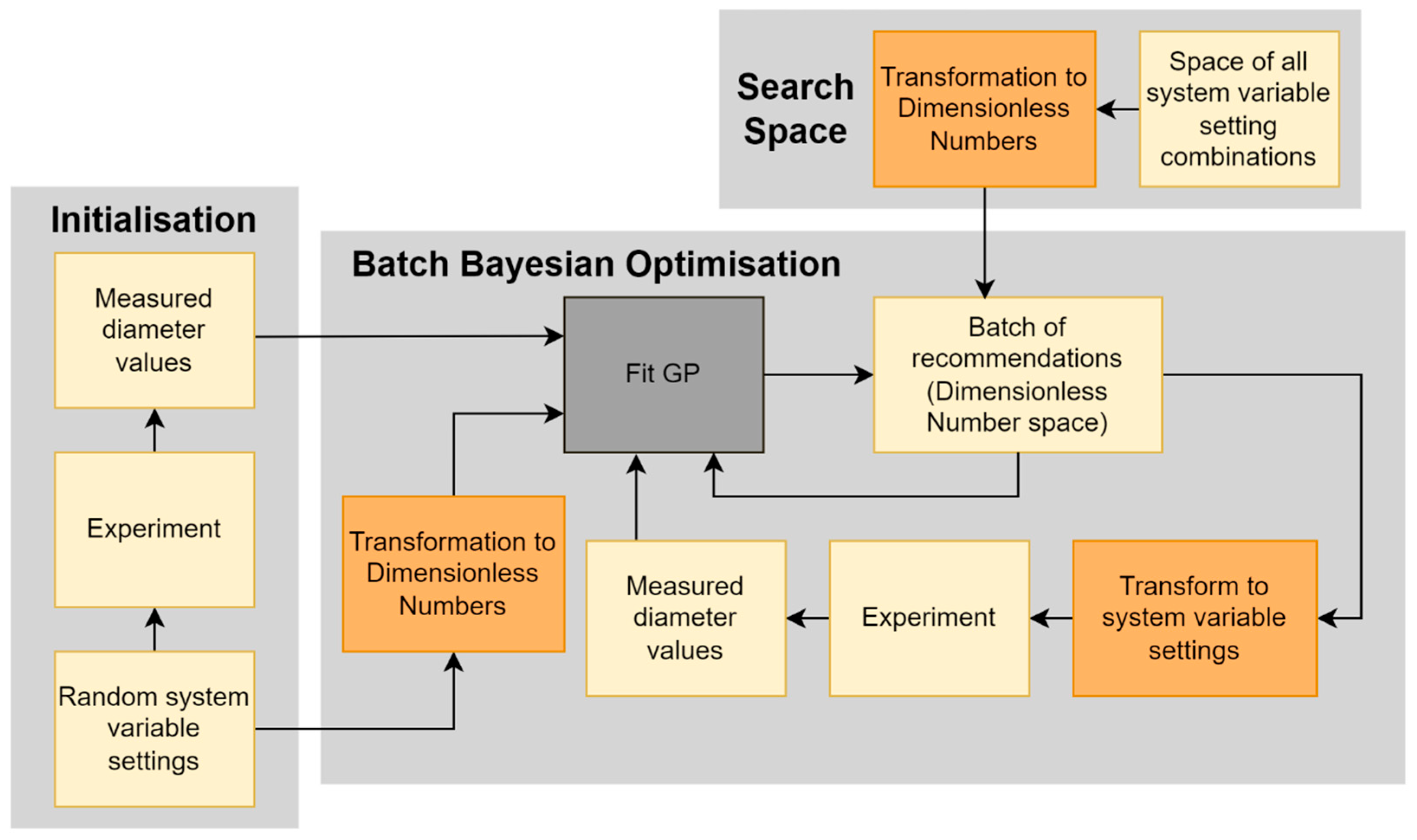
The experimental setup was defined and described in terms of variables and their units for exploitation by the machine. An algorithm was used to derive dimensionless numbers according to the Buckingham π theorem, building off the Python package “BuckinghamPy” (2021) [15]. The system variables and the dimensionless numbers each formed experimental search spaces that mapped to each other via the dimensionless numbers’ algorithm. A BO search was run using the dimensionless numbers space as variables to recommend each batch of iterative experiments. These recommendations (given in the dimensionless number space) were mapped back to the system variable space in which the experiments were conducted. As the experiments progressed, information about the most important factors of the process was progressively derived from the length scale of the variables in the model. This allowed for statistically consistent comparisons between dimensionless numbers.

3.1. Derivation of the Dimensionless Numbers

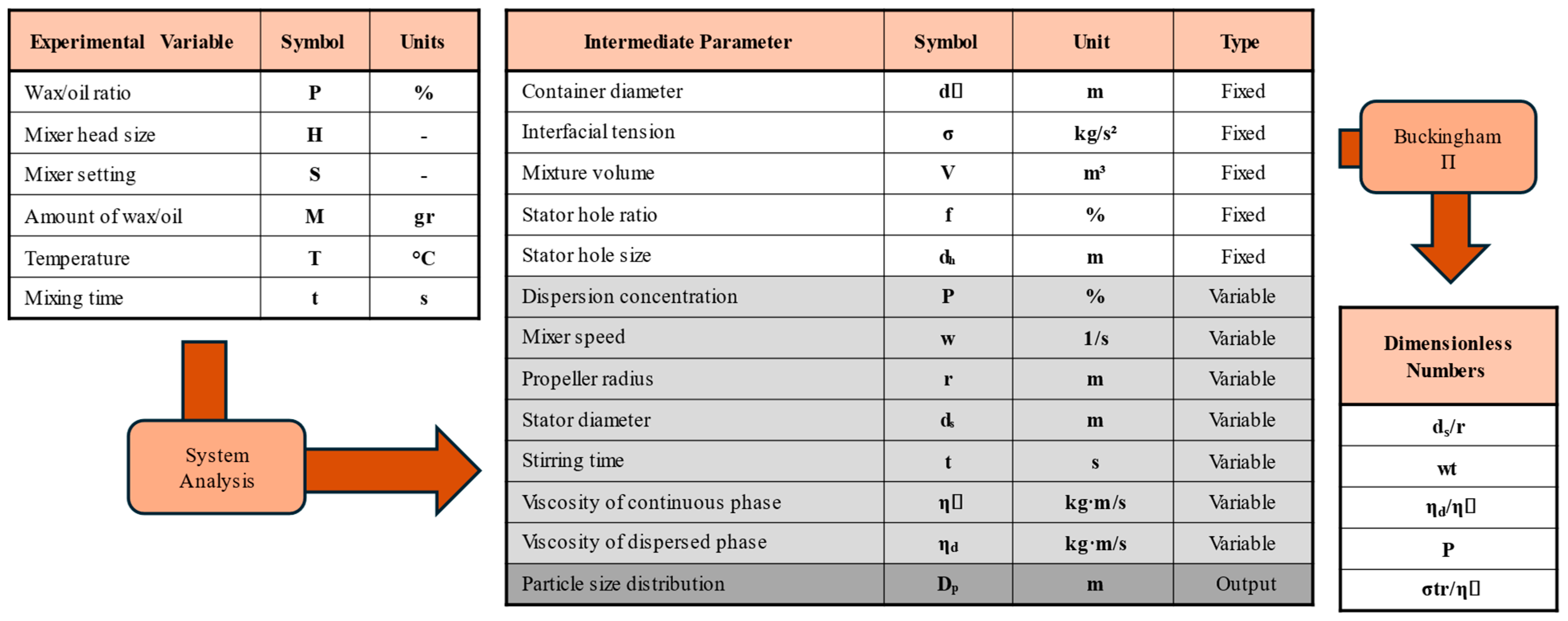
Before the dimensionless numbers were constructed, intermediate parameters were derived using the system variables. These intermediate parameters were then used to construct the dimensionless numbers. Figure 2 lists the system variables, the intermediate parameters, and the dimensionless numbers (via the Buckingham π theorem).

3.2. Batch Bayesian Optimisation for Dimensionless Number Analysis and Particle Diameter Minimisation

Bayesian optimisation, using Python 3 software and the “SciPy minimise” module, was applied to achieve two objectives concurrently. The first objective was to find the optimal value of the system variables, out of the possible combinations described in Table 1, that minimised the particle diameter d90 values ( D p ). The second objective was to determine the dimensionless variables that are the most influential towards particle diameter.
BO is a sample-efficient search method for the global optimisation of complex black-box systems [16]. The method works by building a probabilistic model of the system and requests experimentation at settings that are most likely to return a promising output value. A Gaussian process (GP) is a commonly used probabilistic model with a smooth, non-parametric form [17]. For this study, the GP model was built in the dimensionless number space. As such, the system variables (a mix of numerical and categorical variables) were transformed into dimensionless variables (all numerical), as was discussed and as shown in Figure 2. Equations (1) and (2) show the formulation of the mean and variance of the GP model, where f is the system response (in the case of our system, this was the particle diameter, D p ) and x is the vector representation of the dimensionless number settings (size 5). The relationship between the dimensionless numbers and the particle diameter was modelled by the squared exponential kernel function (Equation (3)), which is parametrised by a length scale vector ( l ) of size 5, where each dimension of the vector is the length scale for each of the dimensionless variables.
μ x t + 1 = k T K 1 f 1 : t
σ 2 x t + 1 = k x t + 1 , x t + 1 k T K 1 k
where
k x i , x j = exp 1 2 l x i x j 2
K = k x 1 , x 1 k x 1 , x t k x t , x 1 k x t , x t
k = k x t + 1 , x 1 k x t + 1 , x t
Each iteration was conducted in batches of 6 samples and batch BO was applied to recommend the next set of experiments [18,19]. After a starting random batch of experiments (Table 2), the following batches (provided as system variables) were suggested by the system. A custom batch Bayesian method was constructed, for which two experiments were recommended for the pursuit of the minimisation of the particle diameter and the remaining four were recommended in the pursuit of maximising the knowledge of the function. The split was selected based on the intuition that allocating more experiments to information maximisation (Objective 2) would in turn support the particle diameter minimisation objective (Objective 1) in subsequent iterations (as better knowledge of the system is obtained) [18]. For the former, we used the Expected Improvement (EI) [20] and GP-UCB-PE algorithm [21]; for the latter, we used variance minimisation [22]. The first point was selected using the EI algorithm (selecting the point that maximises a combination of exploration and exploitation), before using the GP-UCB-PE algorithm to select the remaining points for Objective 1 (in our case, just 1 more). This was carried out by sub-setting the search to those with a high certainty of containing the optima, and from within this, selecting the point with the highest uncertainty (which will result in the highest information gain when sampled). This involved first updating the variance function in Equation (2) with the first point of the batch (found using EI) and maximising the updated variance function. When selecting the set of experiments towards Objective 2, points that had high uncertainty within the GP were selected, as these would lead to being highly informative for the model. High uncertainty can be understood as points that maximise Equation (2). After each new setting for the batch was selected towards Objective 2, the selected point was used to update Equation (2) and the updated version of the variance was used to select the next point. This continued until the batch was complete. These recommendations were made in the dimensionless number space but were transformed into the system variable space for implementation. For the given discretisation of the system variables, each setting, when transformed to the dimensionless number space, was unique, providing a one-to-one mapping that avoided the need for further selection. Had this not been the case, any one of the system variable settings corresponding to the dimensionless number setting could be selected by the experimenter in line with criteria such as the ease of setup or expert hunch. After experimentation at those settings was conducted, the resulting particle diameter (in the form of a d90 value) was returned to the GP model and refitted, with the process repeating until a minimum acceptable diameter was found. This is illustrated in Figure 3.
During this study, the algorithm-derived sets of dimensionless numbers were checked by the experimenter for experimental significance. Otherwise, interactions by the experimenter were minimised to test the system in the most automated way possible. The experimenter’s feedback was sought during the optimisation, but solely to further expand the system variable space in response to the search trends emerging from the algorithm’s exploration of the space.

4. Discussion

4.1. Engineering Approach Aspects

Particle dispersion manufacturing using emulsions of transient melt phases is a widely tackled process in the manufacturing of everyday consumables, including cosmetics, food, and textile formulations. It is a process that is characterised by non-equilibrium states, whereby liquid phases are mixed at a set temperature and subsequently undergo cooling to solidify the dispersed phase. Thermodynamic droplet/particle size stability is typically ensured through use of surfactants, components that minimise interfacial tension and allow smaller particle sizes to be achieved for set mechanical power inputs. While emulsion processing at a constant temperature presents challenges in predicting particle size and stability, processing emulsions across temperature thresholds and phase transition boundaries presents a significant increase in the complexity of the models required for accurate predictions. In systems of this complexity, some additional key parameters may emerge from the subsequent analysis of result dependencies. This is particularly the case in the absence of any surfactant in the system.
The rheological investigations of the wax–oil mixtures in this study indicated a composition-dependent onset of solidification and high dependence on temperature of the measured dynamic viscosity, past the temperature related to the onset of solidification (as shown in Figure S1 of the Supplementary Materials), with the greatest sensitivity being between 60 °C and 66 °C. Above 66 °C, the viscosity of the melt did not appear to differ markedly across compositions. This suggests that varying the operating temperature between 60 °C and 66 °C may yield significantly different particle size distributions if the shear forces applied are equivalent.
Following a random starting set of six experimental conditions, ten batches of six experiments were iteratively suggested by the algorithm for exploration of the space and minimisation of particle size, in response to iteratively provided results. The experiments yielded d90 values below 10 µm with increasing frequency. Experiments were stopped at the 10th batch when d90 values below 10 µm were repeatedly obtained and sufficient information was gathered on the behaviour of dimensionless numbers. The lowest d90 value obtained was 3.22 µm (with a standard deviation of 1.42 µm). While this is considered to be a reasonably large particle size value for an oil in water emulsions with surfactants, it is to be considered a low value in this case for two reasons: (i) no surfactant was used in the process to reduce interfacial tension and, therefore, the thermodynamically achievable particle size, and (ii) the d90 value describes the 90th percentile upper limit in the volume-weighted particle size distribution, which is a widely accepted as being “not larger than” the, or the upper ceiling value for the particle size.
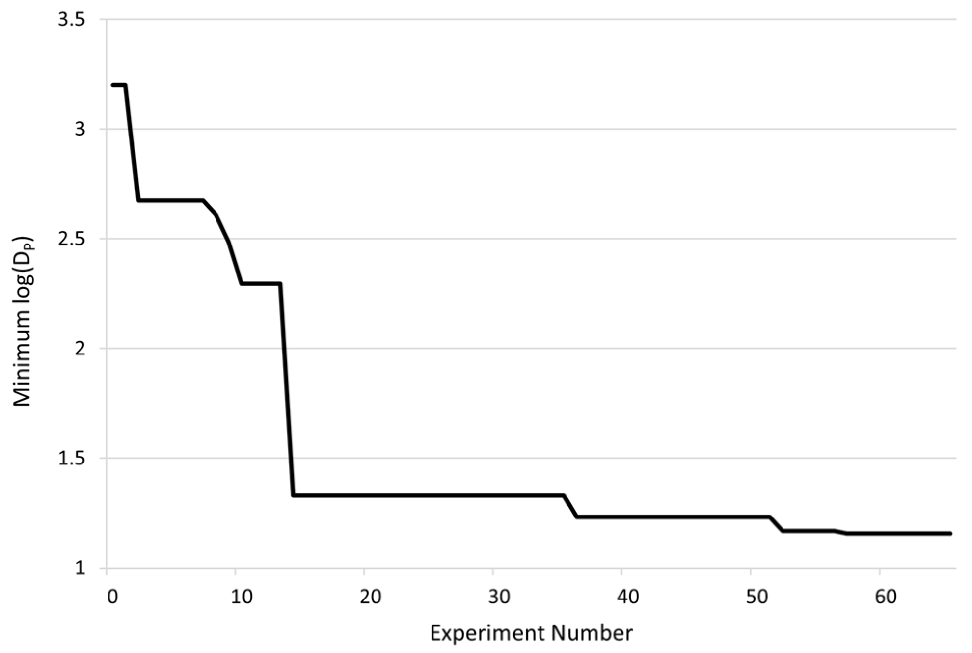
Deciding when to stop experimentation is expectedly difficult if the optimal desired value is unknown. In situations such as this experiment, where it is not possible to know with certainty whether the minimum particle size achievable (optimum for the search) has been reached, the decision to end experimentation is even more difficult. Often, the decision is driven by the depletion of the experimentation budget (cost of experimentation in terms of materials, time, personnel, etc.). However, by observing the relative improvement in the best observation thus far (smallest particle diameter thus far), one can evaluate whether the optimum of the system is close to being reached. Figure 4 shows the smallest particle diameter found after each experiment. In the beginning, large reductions in the particle size (d90 value) can be observed, but the trend tails off, indicating the optimum may have been reached or may be close to being reached. At this point, decoupling the physical experimentation from the BO process-driven suggestions could be beneficial. In this situation, the information held by the experimenter (experience in emulsion systems, knowledge of thermodynamics, etc.) may yield greater improvements with lower experimental costs than continuing with BO-driven exploration of the space.
The second objective of this study was to determine the sensitivity of the results to dimensionless variables. For this, the tuned length scale values of each of the variables in the GP were used as a reflection of sensitivity, with smaller values indicating a stronger sensitivity [23,24]. Tuning of the length scale vector ( l ) was carried out via Maximum Likelihood estimation [25]. The sensitivity of a variable was computed as the inverse of its kernel length scale. In each iteration, as the GP was refitted with the incoming data, the length scale values of the kernel was optimised by maximising the data likelihood [23].
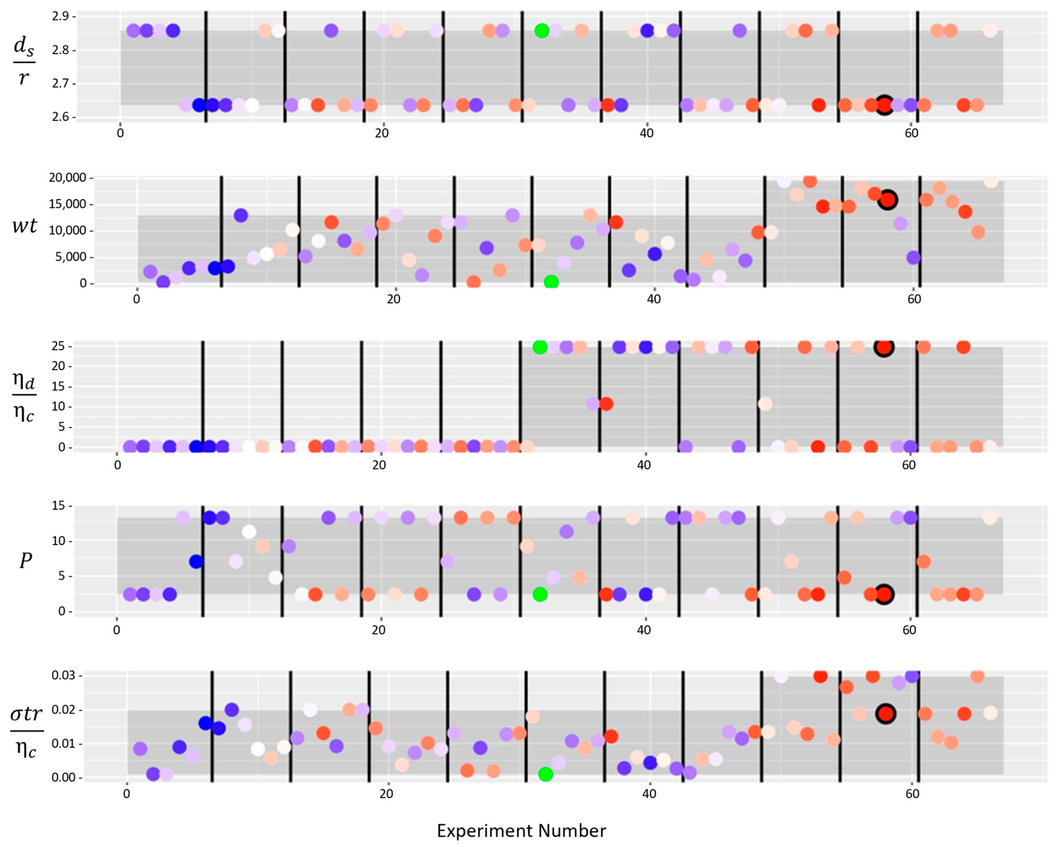
Table 3 describes the length scale values in each iteration, with the dimensionless numbers w t   and σ t r n c resulting as the most influential of the d90 values for particle diameter. The relationship between the different dimensionless numbers and the quality of the samples and its evolution along the optimisation process can be observed in Figure 5. It can be observed that only some dimensionless numbers showed very fine granularity in the length scale values. This is likely related to the array of available system variable values and should not be taken as being reflective of the physics of the system. The coarse step size in some of the system variables resulted in a coarse resolution of the dimensionless parameters ( d s r , n d n c and p ). This can impact the length scales determined by the GP for these dimensionless parameters. A coarse step size may result in a less than required resolution to capture any high-frequency fluctuation of the underlying function and, thus, it can lead to incorrect conclusions such as predicting a higher length scale than in actuality. As such, in this case, a strong conclusion cannot be made as to whether the resulting length scales after tuning truly reflect the informativeness of these parameters to the output. However, in the case that the relationship between the parameter and the output is linear, the length scale of the GP will still be correct. An additional cause for concern is when the grid spacing of the GP’s search space parameters are highly uneven (as is the case for dimensionless parameter n d n c ). In this situation, the length scale estimation may also become inaccurate.
The evolving length scale values provide more than an optimisation trace—they reflect the changing influence of each dimensionless group on the process behaviour. The progression of the particle size optimisation process plotted in Figure 4 shows the particle diameter (d90 value) achieved in each experiment in each iteration within the dimensionless number space. Smaller particle sizes are identified by red dots while larger diameters are shown in blue. The smallest found d90 value is circled in black. The point highlighted in green could not be measured and, as such, was approximated through the average of the other experiments.
This study demonstrated optimisation and searching as a collaboration between an experimenter and the algorithm. At various points in time (i.e., after the 4th and 7th BO iteration) changes were made to the system variable space. This decision was made by the experimenter based on their domain knowledge, ultimately leading to better system outcomes (with the smallest particle diameter found following the second region extension). This further illustrates the flexibility of the Bayesian optimisation search algorithm to be adapted even within a trial. In the case of this experiment, the search space was widened (expanding the range of the system variable values). The final search space (in terms of system variables) is presented in Table 4. Had the search region been reduced, previously observed points that would fall outside the newly bounded region could still have contributed to the estimation of posterior GP, and thus no knowledge would have been lost.
Compared to conducting the experiment in the system variable space, conducting the study in the dimensionless number space was beneficial, as it allowed the identification of both ideal system variable settings (for particle diameter minimisation) as well as uncovering potential sensitive dimensionless variables. Table 5 shows the length scale values (and, as a result, the sensitivity) of the system variables—with low length scale values being reflective of a sensitive variable. Five of the six variables used display some level of sensitivity (compared to just two in the dimensionless space). This reduced number of sensitive variables allows the optimiser to converge faster to the optimal particle diameter region (effectively acting like a lower dimensionality space).
The dimensionless numbers identified as the most impactful in the optimisation of the experiment are w t and p , respectively calculated as (i) the product of time of mixing and frequency of rotation of the impeller, and (ii) the ratio of dispersed mass (mass of added wax/oil mixture) to total mass. The former dimensionless number, w t , is correlated to the power transferred to the mixture and, using this dimensionless number for optimisation in this study, can be considered equivalent to using the integral of energy input over time. As expected, a higher energy input in the mixture tends to favour smaller droplet sizes (d90). The latter dimensionless number can instead be considered to be correlated with two aspects: (i) the volume fraction of the dispersed phase, and (ii) the “resistance” (manifestation of inertial and viscous forces and surface tension) of the dispersed phase as a viscous fluid that resists deformation and breakup into droplets. With all other parameters being kept the same, an increase in the dispersed-to-continuous mass ratio can be expected to result in a greater power input required to attain identical emulsion drop (particle) size distribution, with the total number of drops (hence the total new interface (surface) to be generated) increasing. Another factor related to the volume fraction and mass ratio is emulsion viscosity, which is correlated to them in a non-linear fashion. Emulsion viscosity increased as a direct function of the volume fraction of the dispersed phase, likely resulting from the interaction of dispersed emulsion droplets causing effects similar to particle jamming in high-concentration particle dispersions [26]. The highest value for p in this study is 13.4%, considering a rough 1:1 equivalence of mass ratio to volume fraction. According to the relevant literature, this value is borderline, indicating that the emulsion is likely to be behaving as a free-flow fluid for the large part of the experiments, with minimal impact of the volume ratio on emulsion viscosity [26].

4.2. Regression Trees

More information can also be obtained live, by progressively observing the dependencies between processing variables, dimensionless variables, and experimental results. Specifically, relationships that yield more information on the system’s dynamics can be ascertained. A regression tree was used in this study to further understand the relationships between the dimensionless numbers and the particle diameter.
Due to the coarse resolution of some of the dimensionless numbers, tuning the length scale alone does not provide guaranteed information about relationships. A regression tree is another machine-learning technique to interrogate any relationships.
A regression tree is also an interpretable model. When applied to identify different regions of particle diameter, a regression tree can be used to clearly articulate the ranges of various dimensionless parameters that encapsulate the region resulting in the smallest particle diameters.
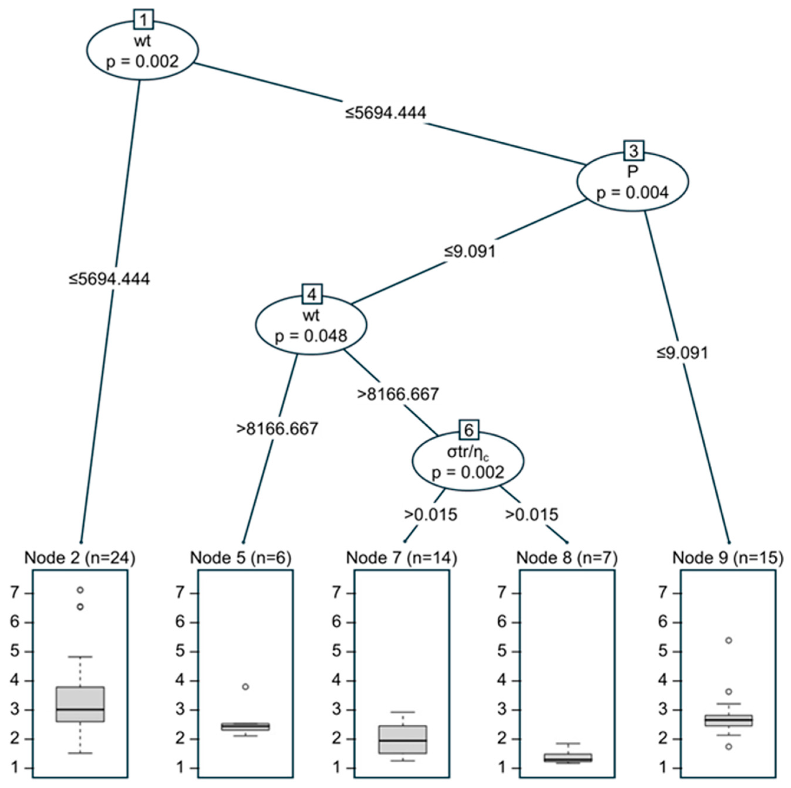
Figure 6 shows the results of this tree, with the critical p-value to permit a split set to 0.1. From the tree, the dimensionless numbers w t , p , and σ t r n c bore importance in segmenting the search space. Compared to the length scale analysis shown in Table 3, the regression tree additionally deemed the dimensionless number ‘ p ’ to be significant; ‘ p ’ had shown a large length scale and had been deemed to be not significant, as discussed above. However, the lack of a small length scale being associated with this dimensionless number can be attributed to the coarse search space of this parameter (as shown in Figure S2 of the Supplementary Materials). This can be contrasted to the fine granularity of the search space of the other two dimensionless numbers. Based on these parameters, a region bounded as described in Table 6 is found to contain the smallest particle diameters. Figure 7 is a three-dimensional scatterplot of these three dimensionless numbers against the diameter of the sampled particles (the diameter of the particle is depicted by the size of the dots). It can be seen that the region bounded by the regression tree (regions with high value for w t and σ t r n c , and low values of p ) contains smaller particles than other areas.
Despite the use of the regression tree, the GP is still a more useful model for sampling, as it can provide a consistent and calibrated estimate of epistemic uncertainty of its predictions [27]. With this, the GP can provide an effective balance of exploration and exploitation for selecting which system variable settings to sample at. Decision trees, at best, can only model aleatoric uncertainty, and would thus not be useful for Bayesian optimisation.
Bayesian optimisation, however, has some limitations that may not make it the most suitable option for some problem settings. These limitations include the following:
  • Difficulty tuning an appropriate length scale for GP for dimensionless parameters that have a coarse resolution;
  • BO is more suitable for small data problems, as fitting a GP with a large amount of data becomes difficult (inversion of the matrix). BO is mostly suitable when the number of data points are relatively small (typically 100–1000 s) and can struggle with numerical precision beyond that;
  • Choosing the correct parameters, such as kernels and kernel hyper-parameters, for a Gaussian process can be difficult and requires several samples. Thus, if the starting parameters are far from optimal, then, in the beginning, BO, without the experimenter’s input, can sample in a way that may seem almost meaningless to an expert;
  • The complexity of parameter estimation scales with the number of dimensions, which, in turn, can be high. Thus, BO can be difficult to run in high-dimensional problems. In the case of this experiment, there were only five dimensionless parameters. Applying this same process may become difficult with more parameters (>16).
As an upside, using techniques such as information collapse via dimensionless numbers, as demonstrated in this study, may permit the use of BO approaches in systems of higher complexity than when using system variables alone. A potential limitation of our approach is that we concurrently aimed to (1) minimise the particle diameter and (2) gather information about the system. These goals may have been reached faster had we focused on just one at a time, rather than sharing resources between the two. Future research could repeat the experimentation separately for each goal and test whether the same conclusions are reached and after how many iterations.

5. Conclusions

This study demonstrates an experimental optimisation and system analysis approach that combines dimensionless groups (collapsed, yet physically relevant, system information) and machine-learning methods. The approach quickly yielded an accelerated exploration of the experimental space, with optimisation of the results and derivation of further system knowledge even in thermodynamically unstable (transient) systems. Our approach was validated by (1) convergence to the expected sensitive dimensionless numbers, verified through domain expertise, and (2) a small particle diameter being achieved.
A peculiarity of BO systems is that they allow the experimenters to continue to dialogue with them, by input of their own evolving insight during the optimisation; this was achieved in this study, for instance, through experimenter-dictated variations in the search boundaries. The two dimensionless numbers identified through this process as being key are in line with the expected governing forces to be balanced in emulsion manufacturing: viscous deformation forces and surface tension forces.
Beyond improving the optimisation efficiency, the practical benefit of this approach lies in its interpretability. By identifying the dominant balances through dimensionless groups, the experimenter gains not only optimal processing conditions but also transferable understanding of the governing mechanisms. This enables more informed decision-making, reduces reliance on trial and error, and allows scaling or adaptation to related processes without restarting the optimisation from scratch.
The proposed method is highly relevant to industrial settings where scaling laboratory processes to production often fails due to complex, high-dimensional parameter interactions. By reformulating experimental variables into dimensionless numbers, the approach effectively reduces the dimensionality of the optimisation space while retaining the essential physics of the system. This reduction not only accelerates the optimisation process but also ensures that insights obtained at one scale remain valid across others, addressing a key challenge in process transfer from lab to plant. In practice, this approach can be adopted by process engineers, materials scientists, and industrial researchers who need to optimise multi-variable systems with limited experimental budgets or uncertain physical models. It is particularly useful when rapid, interpretable optimisation is required to guide process development, enable scale-up, or support sustainable manufacturing innovation.

Supplementary Materials

The following supporting information can be downloaded at: https://www.mdpi.com/article/10.3390/app152212215/s1, Figure S1: Measured Viscosity for wax-oil mixtures at various oil percentages (w/w); Figure S2: Discrete values of the search space for each dimensionless number, related to their capacity to fine tune the system.

Author Contributions

Conceptualization, S.R., S.G., S.V. and A.S.; Methodology, M.S., D.R.d.C.L., S.R., S.S. and A.S.; Software, M.S.; Validation, D.R.d.C.L.; Data curation, D.R.d.C.L., S.S. and N.T.; Writing—original draft, D.R.d.C.L.; Writing—review & editing, S.R., S.S., N.T., S.G., S.V. and A.S.; Visualization, M.S.; Supervision, S.R., S.V. and A.S. All authors have read and agreed to the published version of the manuscript.

Funding

This work was supported by Deakin University and, in part, by the Australian Research Council, grant numbers ARC FL170100006, ARC IH140100018, ARC IH210100023, and ARC IC190100034, which supported the salaries, consumables, and equipment use for this project. A. Sutti also holds a position on the Innovation Advisory Board of the HeiQ Group, and within the Department of Defence (Australia), but only performed the work described in this manuscript as part of her Deakin University appointment. Employment: this work was performed under Deakin University employment for all authors.

Institutional Review Board Statement

Not applicable.

Informed Consent Statement

Not applicable.

Data Availability Statement

The data that supports the findings of this study is available from the corresponding author upon request.

Acknowledgments

This research was supported by the Australian Government through the Australian Research Council Industrial Transformation Research Hub for Future Fibres (IH210100023 and IH140100018), the ARC Research Council Industrial Transformation Training Centre for Green Chemistry in Manufacturing (IC190100034), and the Australian Research Council Laureate Fellowship (FL170100006), of which Venkatesh was the recipient. This study was performed in part at the Deakin Hub in the Victorian Node of the Australian National Fabrication Facility (ANFF). The authors acknowledge Teo Slezak, Marzieh Parhizkar, and Dominic Renggli for their contributions in the form of helpful seeding discussions and help in performing microscopy and preparing the figures. The authors acknowledge Murray J. Height for their helpful seeding discussions. The authors also acknowledge Deakin University’s Advanced Characterisation Facility.

Conflicts of Interest

Author Alessandra Sutti was employed by the company HeiQ Pty Ltd. The remaining authors declare that the research was conducted in the absence of any commercial or financial relationships that could be construed as a potential conflict of interest.

References

  1. Utada, A.S.; Chu, L.Y.; Fernandez-Nieves, A.; Link, D.R.; Holtze, C.; Weitz, D.A. Dripping, Jetting, Drops, and Wetting: The Magic of Microfluidics. MRS Bull. 2007, 32, 702–708. [Google Scholar] [CrossRef]
  2. Eggersdorfer, M.L.; Seybold, H.; Ofner, A.; Weitz, D.A.; Studart, A.R. Wetting controls of droplet formation in step emulsification. Proc. Natl. Acad. Sci. USA 2018, 115, 9479–9484. [Google Scholar] [CrossRef]
  3. Ravishankar, P.; Khang, A.; Laredo, M.; Balachandran, K. Using Dimensionless Numbers to Predict Centrifugal Jet-Spun Nanofiber Morphology. J. Nanomater. 2019, 2019, 4639658. [Google Scholar] [CrossRef]
  4. Utada, A.S.; Fernandez-Nieves, A.; Stone, H.A.; Weitz, D.A. Dripping to Jetting Transitions in Coflowing Liquid Streams. Phys. Rev. Lett. 2007, 99, 094502. [Google Scholar] [CrossRef] [PubMed]
  5. Rahmani, R.; Rahnejat, H. Enhanced performance of optimised partially textured load bearing surfaces. Tribol. Int. 2018, 117, 272–282. [Google Scholar] [CrossRef]
  6. Zhu, Y.; Zhang, R.; Zhu, X.; Pan, X.; Short, M.; Liu, L.; Bussemaker, M. Machine learning modelling of sonochemical systems using physically-derived dimensionless groups. Ultrason. Sonochemistry 2025, 122, 107593. [Google Scholar] [CrossRef]
  7. Greenhill, S.; Rana, S.; Gupta, S.; Vellanki, P.; Venkatesh, S. Bayesian Optimization for Adaptive Experimental Design: A Review. IEEE Access 2020, 8, 13937–13948. [Google Scholar] [CrossRef]
  8. Lee, H.; Moon, H.; Lee, J.; Ryu, S. Toward Knowledge-Guided AI for Inverse Design in Manufacturing: A Perspective on Domain, Physics, and Human–AI Synergy. Adv. Intell. Discov. 2025, e2500107. [Google Scholar] [CrossRef]
  9. Karkaria, V.; Goeckner, A.; Zha, R.; Chen, J.; Zhang, J.; Zhu, Q.; Cao, J.; Gao, R.; Chen, W. Towards a digital twin framework in additive manufacturing: Machine learning and Bayesian optimization for time series process optimisation. J. Manuf. Syst. 2024, 75, 322–332. [Google Scholar] [CrossRef]
  10. Khatamsaz, D.; Vela, B.; Singh, P.; Johnson, D.D.; Allaire, D.; Arróyave, R. Multi-objective materials Bayesian optimization with active learning of design constraints: Design of ductile refractory multi-principal-element alloys. Acta Mater. 2022, 236, 118133. [Google Scholar] [CrossRef]
  11. Lei, B.; Kirk, T.Q.; Bhattacharya, A.; Pati, D.; Qian, X.; Arróyave, R.; Mallick, B.K. Bayesian optimisation with adaptive surrogate models for automated experimental design. NPJ Comput. Mater. 2021, 7, 194. [Google Scholar] [CrossRef]
  12. Roussel, R.; Edelen, A.L.; Boltz, T.; Kennedy, D.; Zhang, Z.; Ji, F.; Huang, X.; Ratner, D.; Garcia, A.S.; Xu, C.; et al. Bayesian optimization algorithms for accelerator physics. Phys. Rev. Accel. Beams 2024, 27, 084801. [Google Scholar] [CrossRef]
  13. Wang, K.; Dowling, A.W. Bayesian optimisation for chemical products and functional materials. Curr. Opin. Chem. Eng. 2022, 36, 100728. [Google Scholar] [CrossRef]
  14. Paulson, J.; Tsay, C. Bayesian optimization as a flexible and efficient design framework for sustainable process systems. Curr. Opin. Green Sustain. Chem. 2025, 51, 100983. [Google Scholar] [CrossRef]
  15. Karam, M.; Saad, T. BuckinghamPy: A Python software for dimensional analysis. SoftwareX 2021, 16, 100851. [Google Scholar] [CrossRef]
  16. Brochu, E.; Cora, V.M.; Freitas, N.d. A Tutorial on Bayesian Optimization of Expensive Cost Functions, with Application to Active User Modelling and Hierarchical Reinforcement Learning. arXiv 2010, arXiv:1012.2599. [Google Scholar] [CrossRef]
  17. Srinivas, N.; Krause, A.; Kakade, S.M.; Seeger, M.W. Information-Theoretic Regret Bounds for Gaussian Process Optimization in the Bandit Setting. IEEE Trans. Inf. Theory 2012, 58, 3250–3265. [Google Scholar] [CrossRef]
  18. González, J.; Dai, Z.; Hennig, P.; Lawrence, N. Batch Bayesian Optimization via Local Penalization. arXiv 2016, arXiv:1505.08052. [Google Scholar] [CrossRef]
  19. Gupta, S.; Rubin, D.; Sutti, A.; Dorin, T.; Height, M.; Sanders, P.; Venkatesh, S. Process-constrained batch Bayesian optimisation. Adv. Neural Inf. Process. Syst. 2017, 30, 3417–3426. Available online: https://dl.acm.org/doi/10.5555/3294996.3295100 (accessed on 9 November 2025).
  20. Wilson, J.; Hutter, F.; Deisenroth, M. Maximizing acquisition functions for Bayesian optimization. arXiv 2018, arXiv:1805.10196. [Google Scholar] [CrossRef]
  21. Contal, E.; Buffoni, D.; Robicquet, A.; Vayatis, N. Parallel Gaussian Process Optimization with Upper Confidence Bound and Pure Exploration. In Lecture Notes in Computer Science; Springer: New York, NY, USA, 2013; Volume 8188. [Google Scholar] [CrossRef]
  22. Yue, X.; Wen, Y.; Hunt, J.H.; Shi, J. Active Learning for Gaussian Process Considering Uncertainties With Application to Shape Control of Composite Fuselage. IEEE Trans. Autom. Sci. Eng. 2021, 18, 36–46. [Google Scholar] [CrossRef]
  23. Rasmussen, C.E.; Williams, C.K.I. Gaussian Processes for Machine Learning; MIT Press Academic: Cambridge, MA, USA, 2005. [Google Scholar]
  24. Seeger, M. Bayesian model selection for Support Vector machines, Gaussian processes and other kernel classifiers. Adv. Neural Inf. Process. Syst. 1999, 12. Available online: https://proceedings.neurips.cc/paper_files/paper/1999/file/404dcc91b2aeaa7caa47487d1483e48a-Paper.pdf (accessed on 9 November 2025).
  25. Bishop, C.M.; Nasrabadi, N.M. Pattern Recognition and Machine Learning; Springer: New York, NY, USA, 2006; Volume 4, p. 738. [Google Scholar]
  26. Liu, C.; Li, M.; Han, R.; Li, J.; Liu, C. Rheology of Water-in-Oil Emulsions with Different Drop Sizes. J. Dispers. Sci. Technol. 2016, 37, 333–344. [Google Scholar] [CrossRef]
  27. Carbone, M.R. When not to use machine learning: A perspective on potential and limitations. MRS Bull. 2022, 47, 968–974. [Google Scholar] [CrossRef]
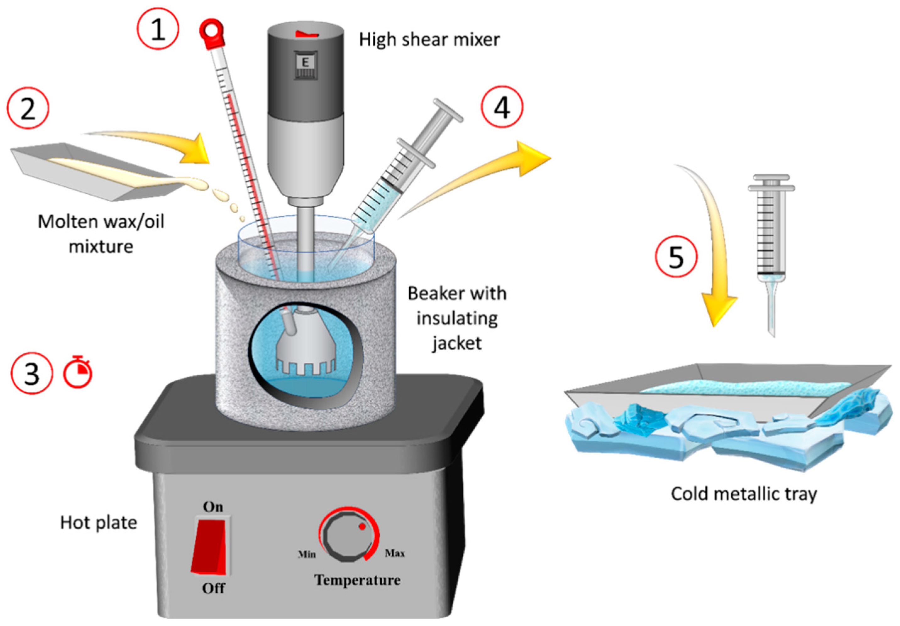
Figure 1. Diagram of the setup used to produce wax/oil emulsions in water. The experiments consist of five main steps, as shown in the diagram: (1) the temperatures of the wax/oil mixture, the water in the beaker with the high shear mixer, and the cold metallic tray are stabilised; (2) the wax/oil mixture is added into the beaker with the mixer applying shear and (3) agitation is maintained for a variable amount of time; a sample of the resulting emulsion is then (4) extracted from the beaker and (5) rapidly added into the cold metallic tray for quenching. Cooled emulsions are then collected and characterised.
Applsci 15 12215 g001
Figure 2. Dimensionless numbers derivation.
Applsci 15 12215 g002
Figure 3. Batch Bayesian optimisation workflow. System variables were converted into their corresponding dimensionless numbers (orange) to perform the search in the dimensionless space. Recommended settings were then mapped back to system variables for experimentation. The resulting particle diameters and associated dimensionless numbers were fed back into the model to update the Gaussian process and guide subsequent batches.
Applsci 15 12215 g003
Figure 4. Smallest log(Dp) value progressively obtained. Experimentation was terminated as the relative reduction in particle diameter had begun to plateau, indicating convergence of the optimisation process and proximity to the system’s performance limit.
Applsci 15 12215 g004
Figure 5. Results from experimental batches (6 each). Red indicates experiments with small particle diameter and blue with large particle diameter. Point circled in black (iteration10) is experimental setting with lowest particle diameter (optimal). Green point (iteration 6) was unable to be measured and was approximated as an average of other experiments. Grey regions indicate available range for each dimensionless variable.
Applsci 15 12215 g005
Figure 6. Regression tree of experimental data. Conducted with a critical p-value = 0.1, the tree has revealed the importance of the three dimensionless numbers (wt, p, σ t r n c ) in segregating the space and identifying a region with small particle diameters.
Applsci 15 12215 g006
Figure 7. A 3D scatter plot of three most significant dimensionless numbers. Dot size and colour reflect the d90 value (logarithmic scale) for the samples. This figure is a stereogram and therefore by viewing each side with the respective eye (parallel view), the figure can be perceived as a 3D model.
Applsci 15 12215 g007
Table 1. Space of possible experimental settings (start of experimentation).
VariableSymbolUnitsStepsSettings
Wax/oil ratioP%601020304050
Mixer head sizeH-2sB
Mixer settingS-7ABCDEFG
Amount of wax/oilMgr651015202530
TemperatureT°C760657075808590
Mixing timets102468101214161820
Table 2. Initial batch of random experimental settings to begin the search algorithm.
Sample IDWax/Oil RatioMixer Head SizeMixer SettingAmount of Wax/OilTemperatureMixing Time
(P, %)(H)(S)(M, gr)(T, °C)(t, s)
120SA58514
20SA5652
320SG5652
40SA57018
50BD30708
640BA158018
Table 3. Length scale of each dimensionless variable in each iteration after fitting GP. Length scale values were constrained to range between 0.01 and 0.6. Low length scale values indicate sensitive parameters.
Iteration d s r w t n d n c p σ t r n c
00.60.01000.600.60.6000
10.60.03070.600.60.1792
20.60.03690.600.60.2284
30.60.04230.600.60.2483
40.60.04230.080.60.2455
50.60.04110.600.60.2487
60.60.04060.600.60.2551
70.60.02490.600.60.1649
80.60.02420.600.60.1646
90.60.02470.600.60.1785
100.60.03590.600.60.5113
Table 4. Space of possible system variable settings (by the end of experimentation).
VariableSymbolUnitsStepsSettings
Wax/oil ratioO%601020304050
Mixer head sizeS-2sB
Mixer settingH-7ABCDEFG
Amount of wax/oilMgr651015202530
TemperatureT°C760657075808590
Stirring timets1024681012141618202224262830
Table 5. Length scales of system variables. Length scale values were constrained to range between 0.01 and 0.6. Low length scale values indicate sensitive parameters.
OH (Encoded)SmTt
0.60.09860.23220.07560.28170.0127
Table 6. Bounds of region with smallest diameter particles.
Dimensionless NumberMinimumMaximum
wt0.015-
p-9.091
σ t r n c 8166.667-
Disclaimer/Publisher’s Note: The statements, opinions and data contained in all publications are solely those of the individual author(s) and contributor(s) and not of MDPI and/or the editor(s). MDPI and/or the editor(s) disclaim responsibility for any injury to people or property resulting from any ideas, methods, instructions or products referred to in the content.