Article

Gross Calorific Value Estimation in Coal Using Multi-Model FTIR and Machine Learning Approach

by
Arya Vinod
1,
Anup Krishna Prasad
1,2,*,
Sameeksha Mishra
1,3,
Bitan Purkait
1,
Shailayee Mukherjee
1,2,
Anubhav Shukla
1,4,
Bhabesh Chandra Sarkar
2,5 and
Atul Kumar Varma
6,7
1
Photogeology and Image Processing Laboratory, Department of Applied Geology, Indian Institute of Technology (Indian School of Mines), Dhanbad 826004, India
2
Geo-Computational and GIS Laboratory, Department of Applied Geology, Indian Institute of Technology (Indian School of Mines), Dhanbad 826004, India
3
CSIR—Central Institute of Mining and Fuel Research, Dhanbad 826015, India
4
School of Earth, Ocean and Climate Sciences, Indian Institute of Technology, Bhubaneswar, Argul, Khorda 752050, India
5
Department of Earth Sciences, Indian Institute of Technology, Bombay, Mumbai 400076, India
6
Coal Geology and Organic Petrology Laboratory, Department of Applied Geology, Indian Institute of Technology (Indian School of Mines), Dhanbad 826004, India
7
Indian Institute of Petroleum and Energy (IIPE), Visakhapatnam 530003, India
*
Author to whom correspondence should be addressed.
Appl. Sci. 2025, 15(22), 12209; https://doi.org/10.3390/app152212209
Submission received: 9 October 2025 / Revised: 10 November 2025 / Accepted: 12 November 2025 / Published: 18 November 2025

Abstract

The Gross Calorific Value (GCV) is a key indicator used to assess the energy potential and quality of coal. Conventional oxygen bomb calorimetry, though widely used, is inherently time-consuming due to the combustion process involved. Similarly, regression models for GCV prediction based on ultimate or proximate analyses require extensive laboratory procedures and sample preparation. To address these challenges, this study investigates the use of mid-infrared Fourier Transform Infrared (FTIR) spectroscopy coupled with supervised variable selection to enable rapid, non-destructive, and cost-effective assessment of coal properties. In this work, a detailed mid-infrared FTIR spectral analysis of coal was conducted to identify fifty-six selective absorption bands (supervised input variables) sensitive to the organic functional group content in coal, coupled with several machine learning (ML) techniques to model the GCV of coal samples from the Johilla coal basin, India. The ML techniques employed here are piecewise linear regression (PLR), partial least squares regression (PLSR), support vector regression (SVR), random forest regression (RFR), artificial neural networks (ANN), and extreme gradient boosting regression (XGB). A multi-model estimation of GCV using the simple average output of the three models (PLSR, RFR, and XGB) achieved the best predictive performance (R2 = 0.951, RMSE = 19.050%, MBE = 1.420%, MAE = 4.053 cal/g), reflecting strong consistency between predictions and actual measurements. The FTIR-based approach achieves competitive or improved results relative to conventional methods and models documented in prior studies. The GCVs derived through modeling of FTIR data are also statistically proven (using t-test and F-test at alpha = 0.01) to be significantly similar to those of the bomb calorimeter, an industry standard for GCV measurements. Consequently, this novel FTIR-based methodology establishes an efficient, dependable tool for GCV determination that operates independently of conventional techniques, thereby enabling rapid quality assessment critical for industrial applications.

1. Introduction

Coal remains the most abundant global non-renewable energy source, with its demand reaching a record 8.42 billion tonnes in 2022, driven by a 4% year-over-year increase amid the energy crisis [1]. While advanced economies like the EU, US, Korea, Japan, Canada, and Australia are progressively reducing coal reliance in favor of cleaner energy sources, fast-industrializing nations, including China, India, Indonesia, Vietnam, and the Philippines, account for over 70% of the global consumption, mostly powered by needs in the iron and steel industry and thermal power plants. Given coal’s continuing importance in the global energy mix, the development of efficient, low-emission, and sustainable utilization technologies is critical to minimizing its environmental impact.
The Gross Calorific Value (GCV), also referred to as the Higher Heating Value (HHV), is a key determinant of coal quality that quantifies the total heat released during the complete combustion of a unit mass of coal under standardized conditions [2]. It is typically expressed in cal/g or MJ/kg. As the heating value determines the applicability of coal in different industries, the accurate estimation of GCV is essential to enhance its economic efficiency. GCV influences the targeted extraction, pricing, processing and utilization and serves as a key parameter in evaluating boiler heat balance, thermal efficiency, and power plant performance, thereby impacting both design safety and production cost estimations [3].
Traditionally, coal-utilizing industries determine GCV using an oxygen bomb calorimeter, which involves complete combustion of coal in a sealed chamber. Although this method provides high precision, it is labor-intensive, time-consuming, and costly, requiring skilled personnel and extensive sample preparation. Furthermore, its batch processing and portability limitations make it unsuitable for extensive or real-time analyses, and the generation of combustion residues adds environmental concerns.
The structure and resulting properties of coals are significantly influenced by the spatial distribution and relative concentration of their constituent elements (C, H, N, O, and S) [4]. Recognizing this relationship, researchers developed empirical correlation methods to rapidly estimate the heating value of coal without relying on bomb calorimetry. In 1880, Dulong proposed one of the earliest and most widely used equations, which assumes that the total heat released by a fuel corresponds to the heat generated by the complete combustion of its elemental components [5]. Since then, numerous modified versions of Dulong’s equation and related correlations have been proposed, each incorporating different assumptions regarding the interrelationships among oxygen, hydrogen, and carbon, as well as the amount of air required for complete combustion.
Subsequent studies developed and refined correlation models to predict the GCV of coal based on ultimate analysis and ash yield, particularly for North American coals [6,7]. A comprehensive review of these early equations later led to the formulation of a unified correlation for HHV derived from elemental composition and ash content [8]. Parallel efforts explored proximate analysis-based correlations, such as a newly proposed empirical relation for estimating the GCV of Turkish lignites [9]. Further correlations were extended to carbonaceous materials, biomass fuels, and their pyrolysis products [10,11,12,13]. In 2008, Majumder et al. [14] developed a simplified proximate analysis-based correlation specifically for Indian coals, improving local prediction accuracy. More recently, the advent of machine learning has enabled advanced regression modeling as an alternative to simple empirical equations, incorporating ultimate, proximate, and hybrid datasets to enhance prediction reliability [15]. However, models relying solely on ultimate or proximate analysis still yield limited accuracy, are costly and time-intensive, and often fail to identify the most influential predictors, resulting in variability and reduced interpretability [16,17].
These limitations have prompted researchers to seek faster, non-destructive, and more reliable alternatives. Spectroscopic techniques, in particular, have gained attention for their ability to directly capture the chemical and structural features of coal. Methods such as laser-induced breakdown spectroscopy (LIBS), near-infrared spectroscopy (NIRS), and X-ray fluorescence (XRF) have all been explored for predicting GCV. Li et al. (2023) used XRF-derived elemental data and proximate analysis to train machine learning models for GCV prediction [17]. LIBS have been coupled with a multivariate dominant factor-based partial least squares model (PLS) [18,19], support vector regression with principal component analysis [20], cluster analysis, artificial neural networks, and genetic algorithms [21,22,23,24] to analyze coal GCV. However, LIBS, as an atomic spectroscopy technique, provides only elemental composition data, limiting its ability to predict coal’s calorific value. It quantifies organic elements (C, H, O, S) to estimate heat value, but carbon analysis is challenging due to interference and low measurement stability. Coal’s complex, inhomogeneous composition amplifies matrix effects, complicating analysis. Experimental parameter optimization and advanced data processing are needed to improve carbon detection. While advancements in LIBS instruments may mitigate these issues, significant progress will take considerable time.
Near-Infrared Spectroscopy (NIRS) provides molecular information and has been widely applied to estimate the GCV content in coal [25,26,27,28,29,30]. In these studies, NIRS reflectance spectra in the visible to near-infrared range were analyzed using various chemometric and machine learning approaches, including PLS-cluster analysis, multiple linear regression, and synergy adaptive-moving window PLS coupled with genetic algorithms. Elemental knowledge from LIBS and molecular evidence from near-infrared reflectance spectroscopy were utilized to optimize the estimation of volatile content and GCV of 45 coal samples from China, spanning the range from lignite to bituminous [31]. However, coal properties exhibit varying correlations with elements and molecules, making spectral interpretation a complex process. NIRS detects overtones and combination bands of the vibrational modes of molecular bonds, which are typically weaker and more complex, often exhibiting broader, less specific bands, making it more challenging to accurately identify organic functional groups [32].
In contrast, mid-infrared spectroscopy offers greater specificity, targeting the fundamental vibrational modes of bonds (like C-H, O-H, and N-H), resulting in distinct sharp absorption bands that are easier to assign to specific functional groups. In 1996, Alciaturi et al. first correlated second-derivative DRIFT (Diffuse Reflectance Infrared Fourier Transform Spectroscopy) spectra with various coal properties, including calorific value, using both multiple linear regression (MLR) and principal components regression (PCR). Their models showed reasonable performance, achieving an R2 of 0.72 and SEP of 1.5 for MLR, and an R2 of 0.54 and SEP of 1.7 for PCR, based on leave-one-out cross-validation [33]. Building on this approach, Alciaturi et al. (1997) applied osculating polynomial-based data compression to infrared spectra, which produced slightly improved correlations for certain coal properties, including calorific value [34]. Two decades later, Roman Gomez et al. (2018) utilized FTIR photoacoustic spectroscopy (FTIR-PAS) coupled with partial least squares (PLS) regression to predict calorific value, achieving strong linear correlations with an SECV of 0.75 MJ kg−1 [35]. In the same year, Qin et al. combined laser-induced breakdown spectroscopy (LIBS) and second-derivative mid-IR FTIR spectra within a PLS framework to predict volatile matter and GCV. Although the fusion model produced R2 values similar to the individual techniques, it notably reduced prediction errors, demonstrating enhanced model robustness [36]. These studies collectively underscore the growing potential of infrared spectroscopy and hybrid models for accurate coal quality prediction, forming the foundation for the present work.
Although previous studies have demonstrated the potential of spectroscopic and hybrid data-driven approaches for GCV estimation, most existing models still depend on complex preprocessing, multi-instrument data fusion, or yield only moderate prediction accuracy. Conventional methods based on proximate or ultimate analyses are also time-consuming, expensive, and often associated with high prediction errors. In contrast, advanced spectroscopic techniques such as LIBS, NIRS, and XRF, while promising, typically require intricate calibration and data integration procedures. Recent studies [37,38,39,40,41,42] have highlighted Fourier Transform Infrared (FTIR) spectroscopy as a single, efficient, and non-destructive tool capable of characterizing multiple coal properties simultaneously. Building upon these advances, the present study develops an integrated framework for GCV estimation using mid-infrared FTIR spectroscopy combined with supervised variable selection and machine learning. The proposed multi-model approach leverages the vibrational signatures of key functional groups to establish robust predictive relationships through algorithms such as piecewise linear regression (PLR), partial least squares regression (PLSR), support vector regression (SVR), random forest regression (RFR), artificial neural networks (ANN), and extreme gradient boosting regression (XGB). This approach achieves higher accuracy, reduced analytical time, and improved cost-effectiveness compared to existing techniques. The overall methodology and validation workflow are illustrated in Figure 1.

2. Materials and Methods

2.1. Coal Sample Data

The Johilla Coalfield in Madhya Pradesh, India, contains sub-bituminous humic coal deposits (G6–G7) essential to regional industries. Following ASTM standards (ASTM D-2234 [43] and D-4749 [44]) 18 coal samples were collected, crushed, and sieved to ~212 μm for FTIR and bomb calorimetry analysis.

2.2. Bomb Calorimetry Analysis

Standard ASTM D-5865 test methods [45] were used to determine the GCV of coal samples. A specific quantity of coal sample was fully burned in a bomb calorimeter to measure the heat released. An automatic bomb calorimeter (Model: HAMCO 6E; Manufacturer: HAMCO, Maharashtra, India; O2 purity: 99.999%) at the Department of Chemical Engineering, National Institute of Technology (NIT) Calicut, Kerala, India, was used to measure the calorific value of the coal samples. The GCV measured using a bomb calorimeter was used as the coal samples’ reference (GCVBC) calorific value.

2.3. Fourier-Transform Infrared (FTIR) Spectroscopy

FTIR spectroscopy is an absorption-based optical molecular analysis technique in which molecules absorb IR radiation and enter higher energy states, causing bond vibrations that produce absorbance peaks at various wavenumbers in the spectrum. These peaks reveal molecular details quickly, safely, and without much sample preparation, making it a valuable tool for coal analysis. The mid-infrared FTIR spectra of samples were used to identify the valid absorption peaks associated with the organic functional groups present in coal. FTIR spectral analysis was performed using an INVENIO S model (BRUKER OPTIK GmbH, Bremen, Germany). Sample pellets used for analysis were prepared by mixing powdered coal of particle size of ~212 µm and potassium bromide (Uvasol powder of IR spectroscopy grade, Merck KGaA, Darmstadt, Germany) [39,40].

2.4. Proximate Analysis

Proximate analysis comprises a series of standardized procedures designed to evaluate the moisture (M), volatile matter (VM), fixed carbon (FC), and ash content (Ash) of coal. Details of the proximate analysis carried out for the samples studied are given in Table 1. For studied samples, moisture values range from 2.0% to 13.8%, with an average of 7.68%. Ash content ranges from 5.0% to 17.8%, with an average of 11.22%. Volatile matter ranges from 24.4% to 32.05% with a mean of 28.03%. The fixed carbon content, representing the solid combustible fraction, ranges from 43.8% to 60.0%, with an average of 53.07%.

2.5. Piecewise Linear Regression (PLR)

Piecewise regression models, with a least squares loss function, enable an iterative search for the best model where the observed values are close to the predicted values if it converges to global minima rather than local minima [46,47,48,49]. A piecewise linear regression model based on quasi-Newton method was implemented to estimate the GCV in coal samples. The model was run with and without breakpoints to generate coefficients for the multivariate regression equation to estimate the GCV.
Two distinct sets of coefficients are generated for the variables when incorporating a breakpoint into the model, QNbp_R and QNbp_L, corresponding to the equations on the right and left sides of the breakpoint. A model is also constructed without a breakpoint, giving a single coefficient form, QNnbp. An average coefficient, QNbp(avg), is calculated by averaging the GCV content estimated from the left and right equations. QNnbp model was found to perform the best and is considered if the predicted GCV from QNnbp falls within the minimum and maximum limit of Q3 + 1.5 IQR and Q1 − 1.5 IQR, respectively. Otherwise, the GCV predicted from the QNbp_avg model will be considered.

2.6. Partial Least Squares Regression (PLSR)

Partial Least Squares Regression (PLSR), or projection to latent structures, extends the multiple linear regression model that adopts a latent variable approach to examine covariance structures between two data spaces. In PLSR, the predictor variables (X) and the response variables (Y) are transformed into a new space called the latent structure. The primary objective of PLSR is to model the covariance between these two matrices by identifying the multidimensional directions within the X-block that best explain the variance in the Y-block. This method is particularly effective when dealing with datasets exhibiting multicollinearity among predictor variables, as it reduces the number of components to an optimal level [50,51]. The model was made with the help of the cross-decomposition module of the scikit-learn library in the python programming environment.

2.7. Random Forest Regression (RFR)

Random Forest Regression (RFR), introduced by Leo Breiman in 2001, is a supervised ensemble learning technique applicable to both regression and classification tasks [52]. It aggregates predictions from multiple decision trees to minimize variance and overcome the overfitting issues common in individual trees, eliminating the need for pruning and improving model stability [53,54]. RFR effectively models complex, nonlinear relationships without assuming predefined dependencies between variables, making it suitable for diverse prediction tasks [17]. In this study, the random forest regressor from the scikit-learn ensemble module in Python 3.12.7 was employed, with hyperparameters optimized using RandomizedSearchCV and GridSearchCV, and the best estimator selected for modeling. The random forest regressor was implemented using the ensemble module of scikit-learn in Python.

2.8. Support Vector Regression (SVR)

Support Vector Regression (SVR), derived from Support Vector Machine (SVM) theory, is a supervised learning approach capable of handling nonlinear and high-dimensional datasets [55,56]. Based on statistical learning principles, SVM constructs an optimal hyperplane that minimizes prediction errors across training samples [57]. Using transductive inference, it efficiently approximates nonlinear functions for quantitative applications such as spectral analysis. In this study, model optimization and training were carried out in Python using the scikit-learn SVM module with GridSearchCV [58].

2.9. Extreme Gradient Boosting (XGB)

XGBoost (Extreme Gradient Boosting) is an advanced machine learning algorithm based on the gradient boosting decision tree ensemble method [54]. It builds regression trees sequentially, where each tree minimizes the residuals of the preceding one, thereby improving model accuracy. Unlike random forests, which construct trees in parallel, XGBoost’s sequential approach is optimized through parallel and distributed computing for faster training [2]. The algorithm controls model complexity at leaf nodes to reduce variance and overfitting, using regularization and an objective function. It further enhances robustness by incorporating first-order gradient information and second-order Taylor expansion for efficient optimization [59,60]. In this study, model optimization and training were performed in Python using the XGBRegressor class with GridSearchCV and RandomizedSearchCV functions.

2.10. Artificial Neural Network (ANN)

Artificial neural networks are versatile machine learning algorithms based on biological beings’ learning mechanisms. ANNs can be envisioned as layers of linked computation units called “neurons” where each link has a specific “weight” based on the type of relationship. Neurons transfer values from input to output neurons, using the weights as intermediate parameters and learning through an iterative process of updating weights connecting the neurons [61]. ANN models train known datasets by adjusting the weights between the mathematical functions and to understand nonlinear associations in large-scale dataset. A “perceptron” is a basic form of a neural network designed to map a set of inputs to an output using an activation function. When several layers of neurons, including multiple hidden layers, are stacked together, the resulting architecture is referred to as a multilayer perceptron (MLP) [55,56]. The ANN model was developed in Python using Keras, a high-level API of the TensorFlow platform [62]. A sequential architecture comprising input, hidden, and output layers with optimized node numbers was constructed, trained, and used to generate predictions.

3. Results

3.1. Gross Calorific Value of Coal Samples

The gross calorific value of all the coal samples measured by bomb calorimetric analysis is reported in calories per gram (cal/g), along with their proximate parameters and statistics, which are given in Table 1.

3.2. Selection of MIR Bands Suitable for GCV Determination

Coal consists of diverse functional groups, including sulfur, oxygen, and nitrogen within its organic framework [63]. The energy deciding the calorific value depends on the spatial distribution and concentration of the elements [4] (mainly carbon, hydrogen, and oxygen), oxidation of organic compounds made from these elements, and the degree of aromatization [38,64] with re-distribution of the aromatic-hydroaromatic carbon matrix [7,65]. FTIR is a widely applied analytical method to examine the structural characteristics of coal. The ability of FTIR to identify the carbo-hydrogenated structures (aromatic and aliphatic) and heteroatomic functions (oxygenated), along with the advantages of rapid analysis and independence from crystal structure constraints, makes it highly effective for coal characterization [38,66]. Based on this principle the present study utilizes easily obtained mid-infrared FTIR input datasets, avoiding more complex analytical tests and combustion of samples.
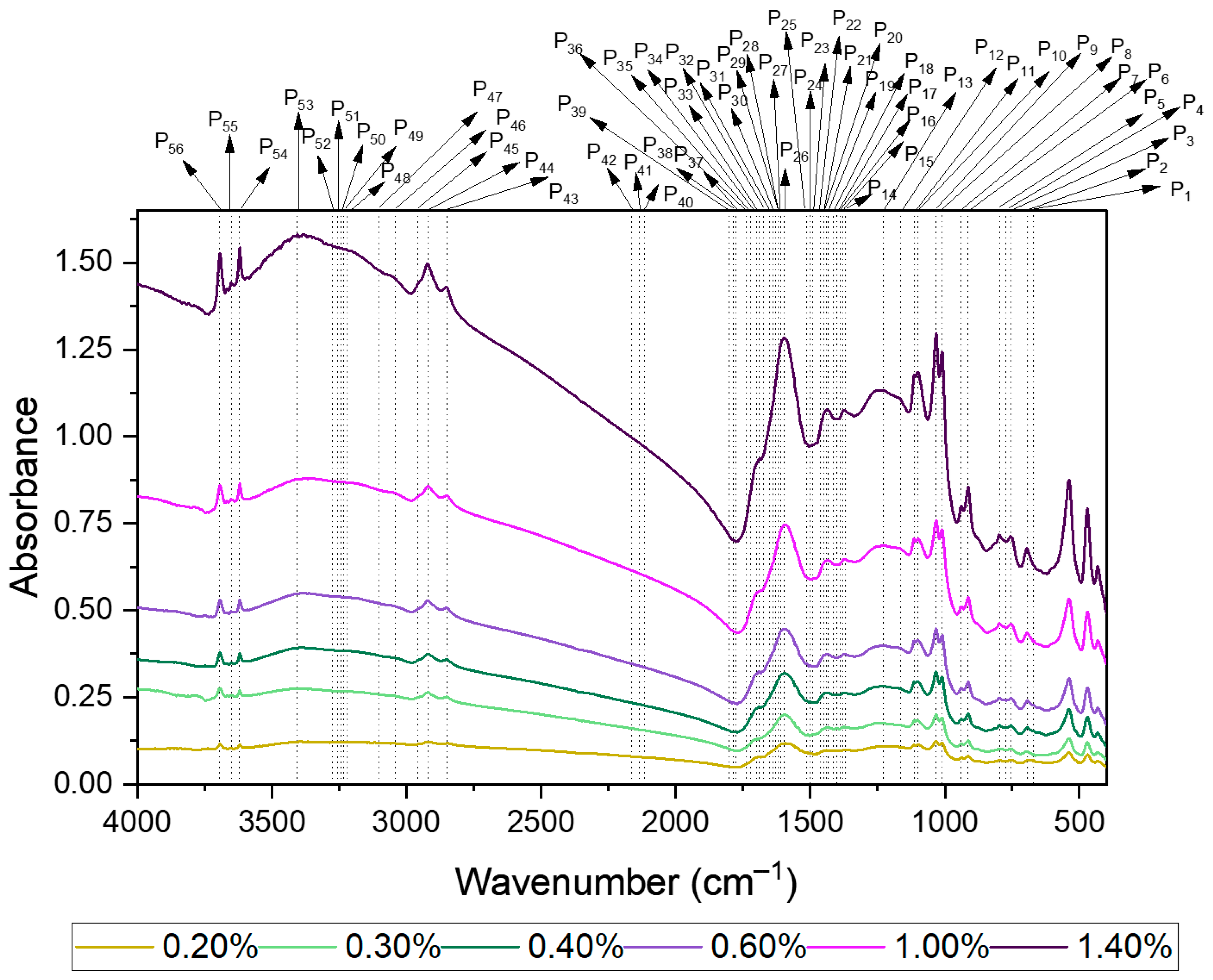
According to the literature [38,66,67], the FTIR spectrum of coal can be broadly categorized into four distinct absorption bands: the 700–900 cm−1 band, corresponding to aromatic hydrocarbon structures; the 1000–1800 cm−1 band, associated with oxygen-containing functional groups and partial aliphatic hydrocarbon (carbon skeleton structures); the 2800–3000 cm−1 band, representing aliphatic hydrocarbon structures; and the 3000–3600 cm−1 band, which corresponds to hydroxyl groups. Figure 2 depicts the systematic variations in the absorbance observed for coal samples at six concentrations in coal + KBr pellets (0.20%, 0.30%, 0.40%, 0.60%,1.00%, and 1.40%), using FTIR for the sample J_13. The location and magnitude of absorption peaks in the FTIR spectrum correlate with the chemical composition and the concentration of functional groups. All the identified peaks, their onset, and offset in wavenumber (cm−1), along with the corresponding functional group, are given in Table 2 and Table 3.
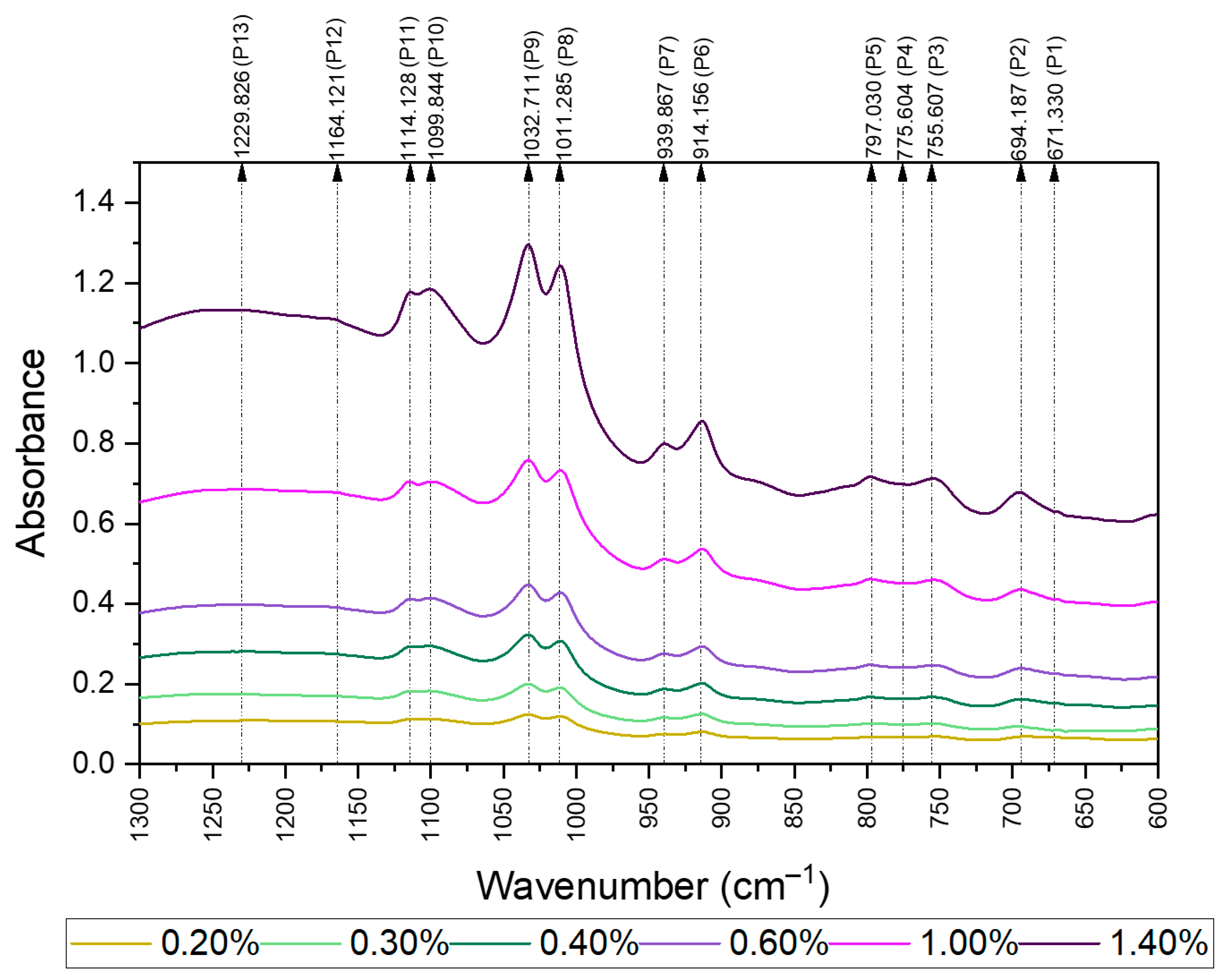
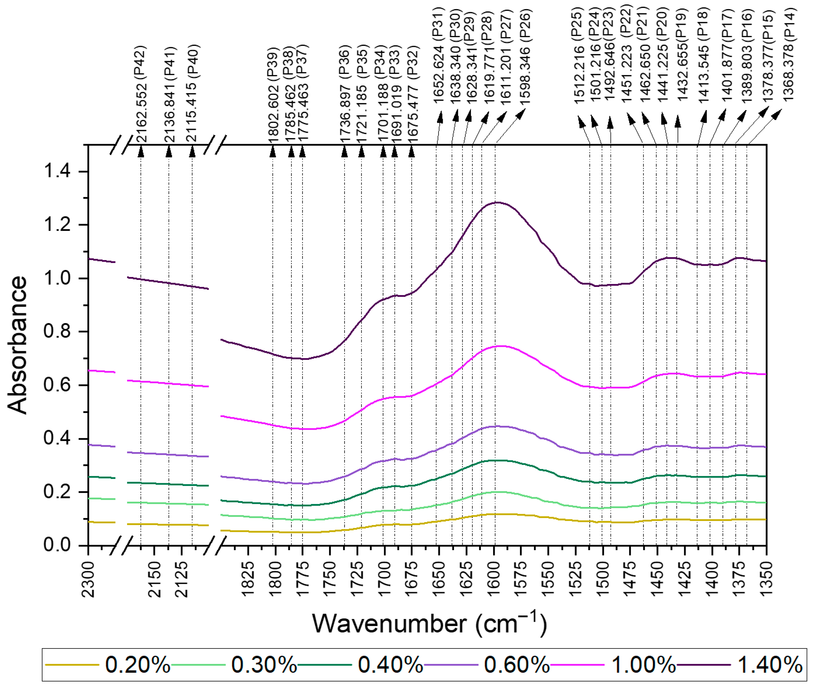
The spike at 671 and 694 cm−1 is ascribed to the stretching modes of the C-S band in thioethers and mercaptans [70,73]. These peaks are given in notations P1 and P2 in Table 2 and Figure 3. Aromatic hydrocarbons are unsaturated hydrocarbons that contain one or more planar six-carbon rings, called benzene rings, with hydrogen atoms. In the FTIR spectrum of coal, the region between 1000 and 700 cm−1 corresponds to the out-of-plane C–H deformation vibrations associated with aromatic structures (CHx). Aromatic ring substitution patterns can be broadly divided into four categories: bands near 900–850 cm−1 are linked to isolated aromatic hydrogen atoms; those in the 850–810 cm−1 range indicate two adjacent hydrogens on the same ring; peaks occurring around 810–750 cm−1 represent three neighboring aromatic hydrogens, denoted as P3, P4, and P5 (Table 2, Figure 3); and absorptions between 750 and 730 cm−1 correspond to four contiguous aromatic hydrogens [66]. Although not a dominant feature in coal, the C–O–C stretching of epoxide groups may appear within 950–810 cm−1 (P6 and P7) [71,72]. Additionally, the spectral interval between 1610 and 1502 cm−1 is attributed to C=C stretching within aromatic and fused ring systems (P24 and P25 in Table 2 and Figure 4).
The FTIR stretching vibration mode of aliphatic moieties of coal samples appears in the 3000–2800 cm−1 range [68] (P43, P44, P45 in Figure 5).
The C–H stretching bands of aliphatic hydrocarbons associated with sp3 hybridization can be distinguished from methene and methylene groups. The absorption zone around 2950 cm−1 (P45) corresponds to the anti-symmetric stretching of methyl groups, while 2920 cm−1 reflects the anti-symmetric stretching of methylene groups (P44). The band at 2850 cm−1 (P43) is attributed to symmetrical methylene stretching. Methine groups are present within the aliphatic chain, connecting saturated alicyclic rings to aromatic rings and branch chains to methyl groups [74].
C–H bending vibrations occur in the range of 1500–1350 cm−1, primarily involving methyl and methylene groups. The CH3 symmetric bending vibration of methyl is observed around 1360 to 1385 cm−1 band (P14, P15) [66]. The C-O-H bending vibration of alcohols and phenols also appears as broad and weak peaks at 1440 to 1380 cm−1 (P16 to P20), mostly obscured by CH3 bending [73].
The stretching vibration for sp2 =C-H occurs in the range of 3120 to 3000 cm−1, while the C=C stretch typically appears between 1660 and 1600 cm−1 (P26 to P31 in Figure 4). Conjugation of the C=C bond lowers the frequency and increases the intensity. Alkynes, containing the C≡C group, exhibit characteristic stretching bands, including ≡C–H and C≡C stretching. The stretch for ≡C-H in sp hybridization occurs between 3300 and 3200 cm−1, while the C≡C stretch is between 2260 and 2100 cm−1. The C-H stretching bands for sp2 carbons of alkenes and aromatic compounds appearing between 3100 and 3000 cm−1, make it difficult to distinguish between aromatic compounds and alkenes based solely on these bands. However, skeletal vibrations, which correspond to C=C stretching in aromatic rings, occurring between ~1500 and 1430 cm−1 (P21 to P25 in Table 2 and Figure 4) can help distinguish them from alkenes [73].
The absorption range for oxygen-containing functional groups in the infrared spectrum of coal samples falls between 1800 and 1000 cm−1. These groups include hydroxyl (OH), carboxyl (–COOH), carbonyl (C=O), and ether (R–O–R’) bonds. Alcohols and phenols, sensitive to hydrogen bonding, show distinct infrared bands due to O–H and C–O stretching, typically in the broad 1300–1000 cm−1 (P8 to P13 in Table 2 and Figure 3) range. Ethers can be identified by their C–O–C bond, which produces a strong C–O stretching band around 1100 cm−1. Specifically, the peak around 1036 cm−1 (P9) corresponds to alkyl ether, while around 1097 cm−1 (P10) indicates aryl ether [38]. The ether bond is a crucial structural element that bridges the principal structural units of condensed aromatic rings in the macromolecular structure of coal.
The peaks relating to C=O and C=C bonds in aldehydes, ketones, carboxylic acids, and esters are shown from P32 to P36. Carbonyl bands appear in the FTIR spectrum at different ranges depending on the type of carbonyl compound. For aldehydes, aliphatic ones produce bands between 1740 and 1720 cm−1, while aromatic aldehydes have bands between 1720 and 1680 cm−1. Similarly, ketones show carbonyl bands between 1730 and 1700 cm−1 for aliphatic ketones and 1700–1680 cm−1 for aromatic ketones [67,73]. Carboxylic acids (RCOOH) often form dimers due to strong hydrogen bonding. When simple aliphatic carboxylic acids are dimeric, they show a broad C=O stretching band between 1730 and 1700 cm−1 [63]. In an ester spectrum, the strongest bands are produced by the two most polar bonds, the C=O and C–O bonds, which are part of the –CO–O–C– unit. Since the C=O stretching and C–O stretching vibrations occur in distinct frequency ranges, aliphatic and aromatic esters can be differentiated. Aliphatic esters show C=O and C–O bands in 1750–1730 cm−1 and 1300–1100 cm−1, respectively. Aromatic esters, on the other hand, exhibit C=O bands between 1730 and 1705 cm−1, with 1727 cm−1 being characteristic of aryl esters [38,63,66]. The peaks from P32 to P36 are shown in Figure 4.
The position of the C=O stretching wavenumber in these zones is affected by factors like hydrogen bonding and conjugation in the molecule. Conjugation with a C=C bond causes the absorption to shift to a lower wavenumber due to the redistribution of electron density in the C=O group. The characteristic carbonyl band can distinguish anhydrides (–CO–O–CO–), which exhibit C=O stretching bands in the 1840–1800 cm−1 and 1780–1740 cm−1 ranges (P37 to P39 in Figure 4). Each band shifts by approximately 30 cm−1 to a lower frequency when conjugated. Additionally, the weak broad band observed at 1030 cm−1 is related to the C-O stretching of phenolic groups.
In the FTIR spectrum of a coal sample, the hydroxyl functional group stretching vibration band appears between 3700 and 3000 cm−1. The 3730−3100 cm−1 spectral band does not mainly interfere with other functional groups and is the most suitable for studying the OH groups in coal. They can form different hydrogen bonds with various acceptors. Hydroxyl groups influence the reactivity of coal, which is crucial in breaking or forming cross-linking bonds and impacting the coal’s natural properties. Hydrogen bonds link distant and compact regions of the network with a greater force than non-specific intermolecular forces, achieving a stable molecular network. The O−H absorption band comprises two sections: the free O−H stretching band in the range 3750–3600 cm−1, as identified as P54, P55, and P56 without hydrogen bonds, and a broad O−H stretching band in the 3600–3100 cm−1, as identified as P47 to P53, associated with hydrogen bonds [69] (Figure 5).
The peak around ~3616 cm−1 (P54) represents the stretching vibration of free hydroxyl groups, which occurs when hydrogen bonds cannot form due to steric hindrance or when the bond is very weak [63]. This peak is also linked to crystal water in clay minerals. The stretching vibration at 3220 cm−1 (P48) is associated with cyclic hydrogen bonds. The OH-N hydrogen bond, which forms an acid-base complex between phenol and pyridine, is around 3040 cm−1 (P46).
Using a detailed analysis of peak assignments corresponding to their respective functional groups, the area under the curve was calculated for 56 peaks, as illustrated in Figure 3, Figure 4 and Figure 5.

3.3. Model Estimation and Assessment

Eighteen coal samples were selected for GCV estimation. For each sample, six KBr-diluted pellets were prepared using 220 ± 0.20 mg of KBr with coal concentrations of 0.20%, 0.30%, 0.40%, 0.60%, 1.00%, and 1.40%, yielding a total of 108 pellets. Mid-infrared spectra were recorded using a Bruker FTIR spectrometer in transmission mode over the range 4000–400 cm−1 [39,40]. Baseline correction (spectra of pure KBr were subtracted) was applied to minimize background noise, enhance signal to noise ratio and ensure quantitative accuracy.
Specifically, the area under the curve (AUC) of the above-mentioned fifty-six mid-infrared absorption bands sensitive to the hydrocarbon functional groups in coal, set as independent variables, was fitted using PLR, PLSR, RFR, SVR, XGB, and ANN regression models. K-fold cross-validation (K = 18) was used to evaluate the FTIR-based model’s performance in determining the GCV content. A 17:1 split was applied to one hundred and eight coal sample pellets, grouped into 18 sets (6 pellets per group at known concentrations). During each run, one-fold served as the test set, while the remaining (K-1) folds were used for training, ensuring each fold was tested independently at least once.
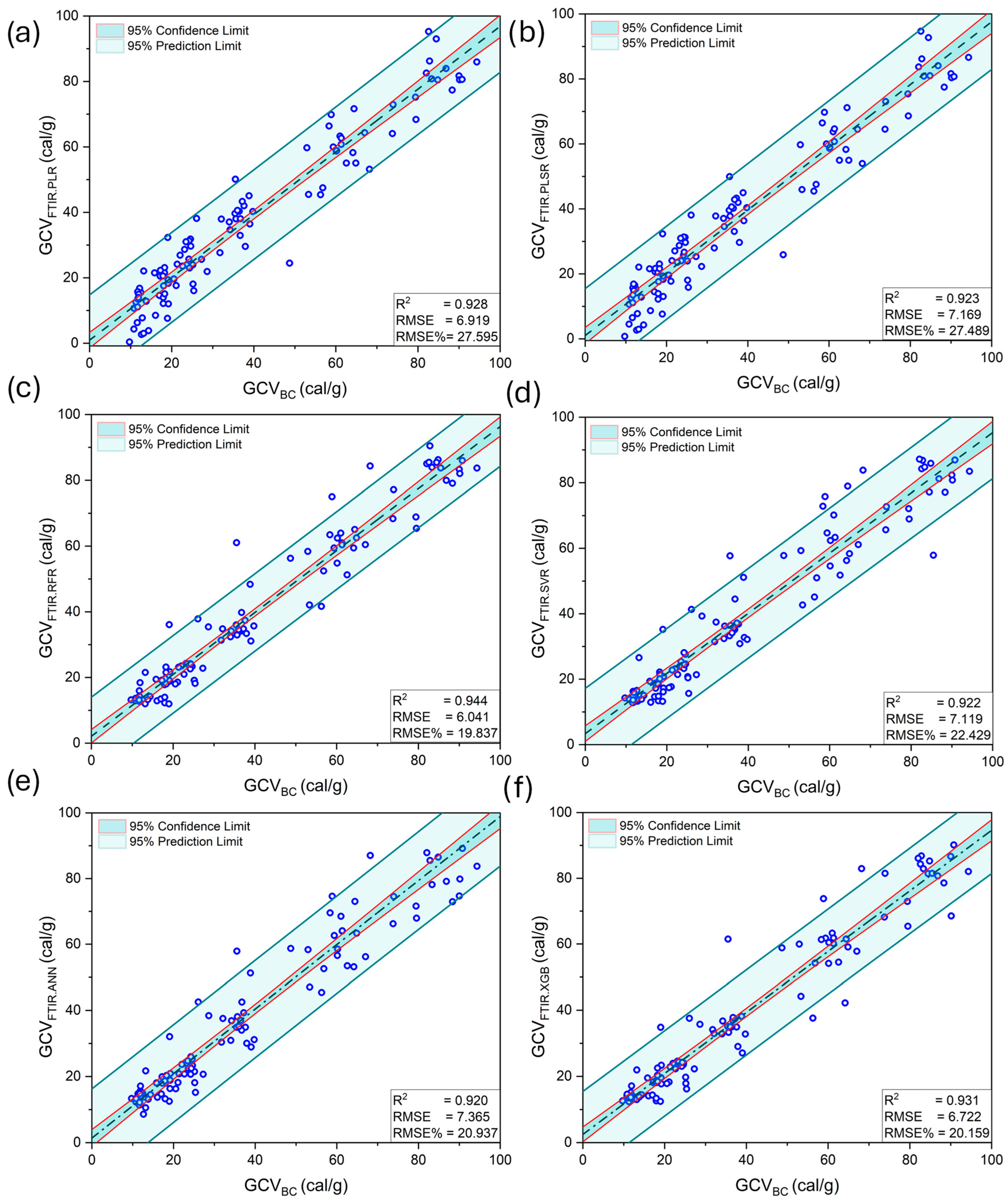
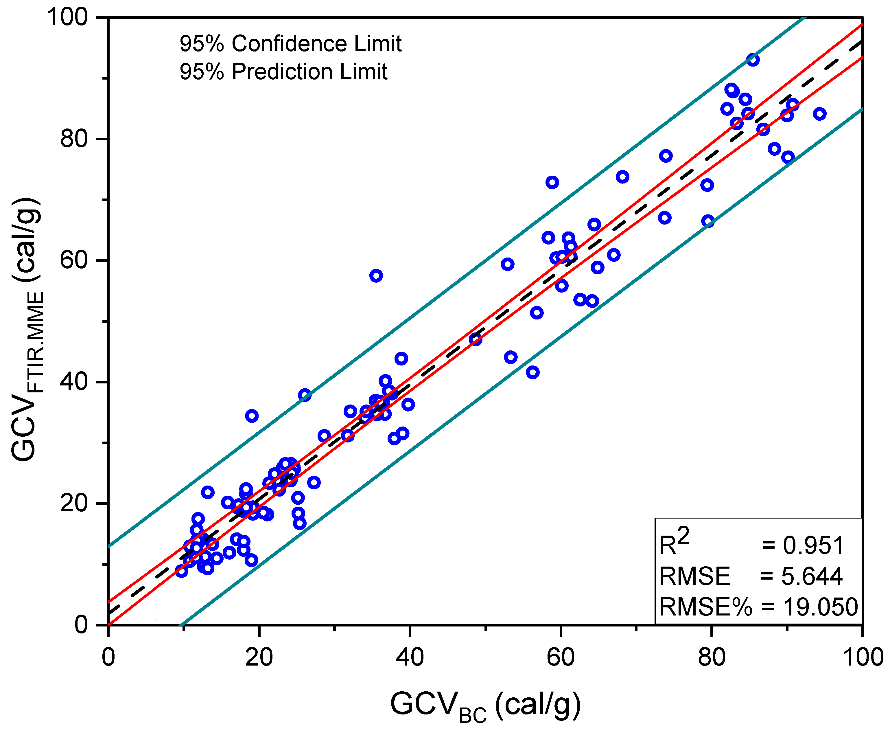
The alignment between the predicted values and the actual values of the six regression models (PLR, PLSR, RFR, SVR, ANN, XGB) is shown in Figure 6. The study adopted six predictive performance evaluation criteria used in regression analysis. These include the coefficient of determination (R2), root mean squared error (RMSE), mean bias error (MBE), and mean absolute error (MAE) of the established models in absolute and percentage values. MBE and MAE are metrics for evaluating errors, with smaller values indicating better model performance. Similarly, an R2 value closer to 1 signifies a superior model fit. The performance of all seven developed models is summarized in Table 4. For MME selection, all possible three-model combinations were explored, averaging their predictions to form ensembles. Each three-model combination was evaluated to identify the optimal ensemble that yielded the best performance with the least error. The PLSR, RFR, and XGB models adopted in this study produce a strong match throughout the data range visually with a R2 value of 0.923, 0.944, 0.931, and an RMSE% of 27.489, 19.837, 20.159, respectively. A multi-model estimation strategy, averaging the results of the three models (PLSR, RFR, XGB), yielded the best fit for the sample data, with the predicted values closely matching the actual values, achieving greater precision and robustness than individual models, as recorded by an R2 value of 0.951, an RMSE value of 5.644 cal/g, an MBE value of −0.336 cal/g, and an MAE value of 4.053 cal/g. The comparison between the model predicted (GCVFTIR_MME) and bomb calorimetry measured (GCVBC) calorific value of coal sample pellets is given in Figure 7. In conclusion, the experimental results demonstrate that the MME model is highly effective in predicting the GCV of coal.
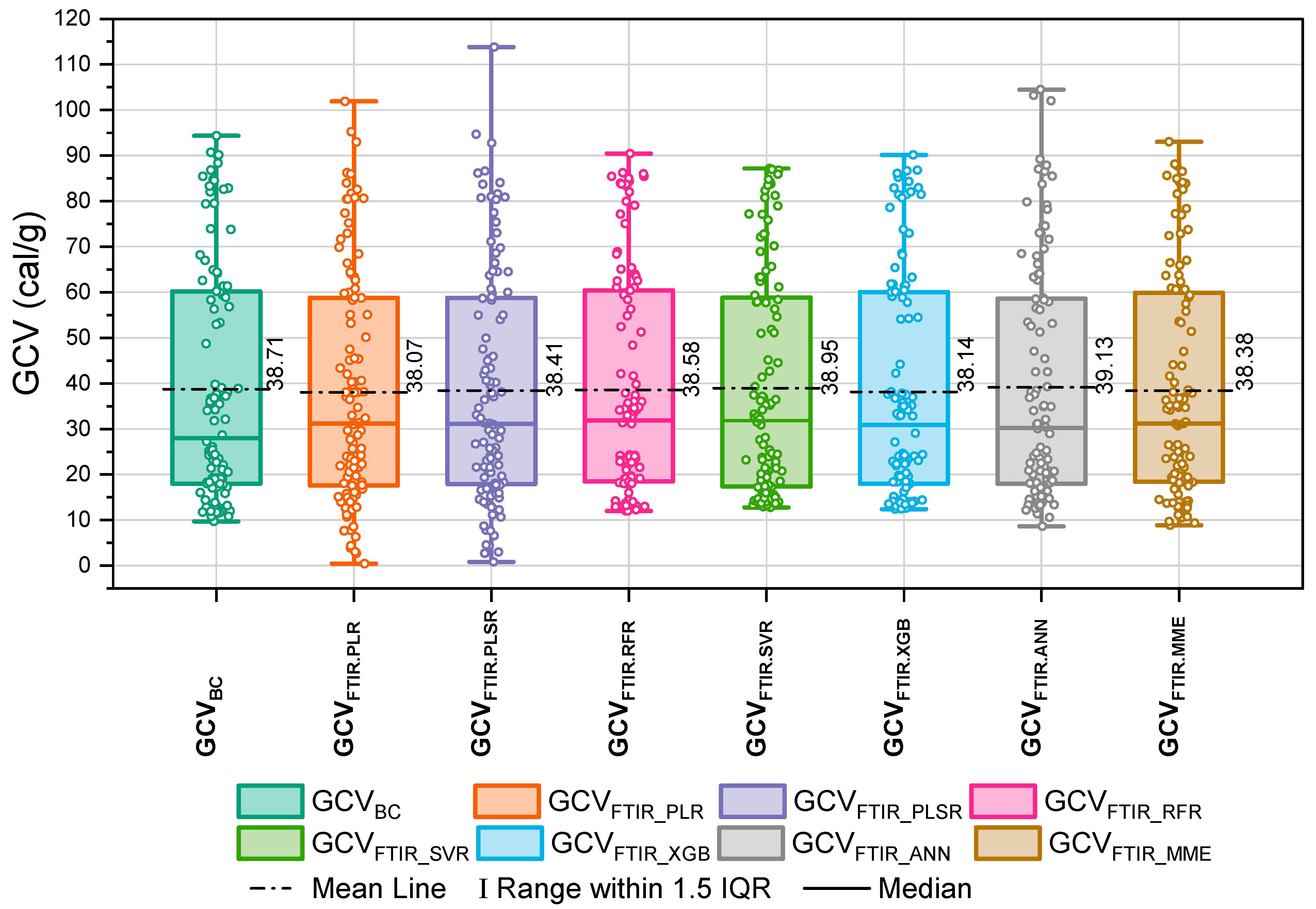
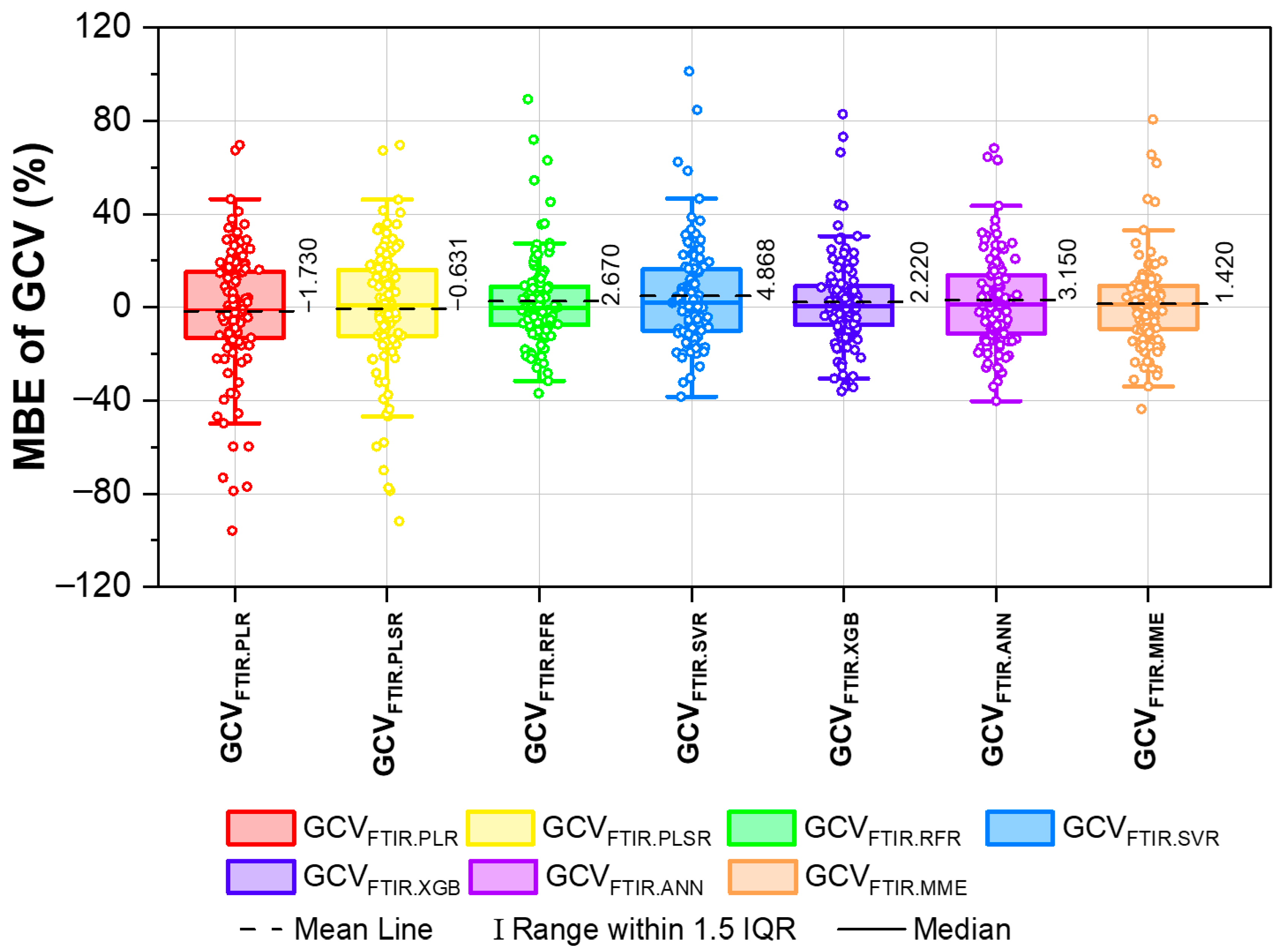
The boxplot depicting the distribution of GCV in coal measured using bomb calorimetry (GCVBC) and by model-prediction (GCVFTIR.PLR, GCVFTIR.PLSR, GCVFTIR.RFR, GCVFTIR.SVR, GCVFTIR.XGB, GCVFTIR.ANN, GCVFTIR.MME) as displayed in Figure 8 does not show any substantial difference in the mean value. Likewise, the MBE % of the proposed models was plotted to illustrate the average bias in each model for coal (Figure 9). The multi-model estimated GCV achieved the least mean bias error of 1.420% which depicts the model’s consistent performance. A Taylor plot is a graphical representation used to assess the performance of different models by comparing their correlation, standard deviation, and RMSE against a reference dataset. Figure 10 presents a Taylor plot to graphically compare the performance of seven models (PLR, PLSR, RFR, SVR, ANN, XGB, and MME) used in the present study in predicting the GCV of coal with respect to the reference bomb calorimetry (BC) data. Models nearest the reference BC point in Figure 10 present better performance, having higher correlation, comparable standard deviation, and lower RMSE. The MME model plots nearest to the BC reference line in Figure 10 and reflects better agreement with actual BC value, thus being more accurate for GCV prediction.
A paired t-test for means and a two-sample F-test for variance conducted at a 99% confidence level accepts the null hypothesis (H0: μd = 0 for t-test; where μd is the hypothesized mean difference and H0: σ2o = σ2p for F-test; where σ2o is the variance of observed data and σ2p is the variance of predicted data). These statistical tests prove that no substantial difference exists between the mean and variance of the GCVs obtained from bomb calorimetry (GCVBC) and those predicted by the model (GCVFTIR.MME) for coal samples. The detailed results of the paired t-test for means and the two-sample F-test for variance are provided in Table 5 and Table 6, respectively.
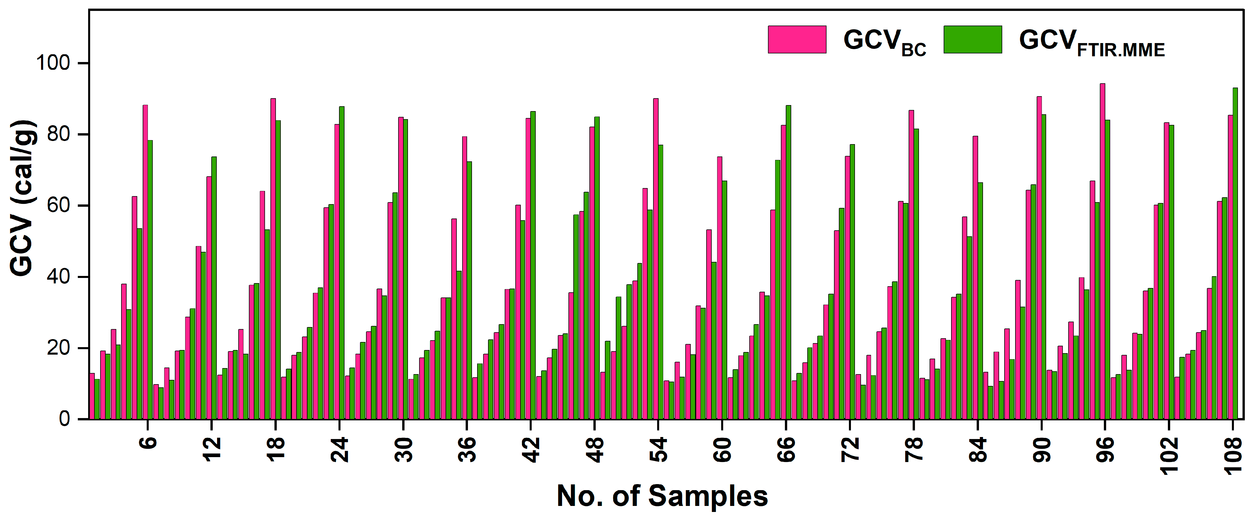
A grouped bar chart illustrating the comparison of the bomb calorimeter measured GCV content (GCVBC, cal/g) and the GCV content predicted from multi-model estimation using FTIR data (GCVFTIR.MME, cal/g) for one hundred and eight coal sample pellets is provided in Figure 11. It can be inferred from the graph that both the datasets show similar distribution and are comparable in nature. Taken together, all results imply that the multi-model approach-based FTIR spectroscopy technique is an innovative, sensitive, and reliable method for predicting the GCV content in coal.

4. Discussion

FTIR analysis provides a cost-effective and user-friendly alternative for estimating the GCV of coal. It eliminates the need for combustion and requires simpler, less expensive instrumentation and consumables. In contrast, an automatic bomb calorimeter analyzes approximately 20 samples continuously, taking nearly 30 min per sample (including preparation and heating), and consumes crucibles, cotton threads, and ignition wires, making it less practical for large-scale analyses. FTIR spectroscopy, which requires only KBr and takes less than 8 min for pellet preparation and spectral acquisition, enables rapid, low-cost, and continuous measurements with comparable accuracy. Its non-destructive nature allows repeated analysis of the same sample. With further refinement, the method can be tailored to include or exclude variables based on coal grades and has strong potential for development into portable or handheld FTIR-based devices for real-time, in-field GCV estimation.
Table 7 presents the comparison of the statistical performance metrics (R2, RMSE, MBE, MAE) between the present study and previously published works using different methods/equipment/input data/algorithms. Models with an R2 value approaching 1, coupled with error measures such as MBE, MAE, and RMSE nearing zero, are universally recognized as highly precise and reliable for accurate estimation [75]. The comparative analysis distinctly demonstrates that the proposed multi-model FTIR-based estimation of GCV often surpasses the predictive accuracy of previously reported models. In particular, the most recent GCV estimation approaches based on proximate and ultimate analyses [76,77,78] show substantially higher error values, reaffirming the superior precision, efficiency, and innovation of the present method. Furthermore, the present study, which utilizes FTIR spectroscopy, will complement previous attempts to estimate coal properties using mid-infrared spectroscopy, enabling the concurrent analysis of several coal properties with a single analytical technique. This could transform the coal industry by significantly reducing analysis time and facilitating quality control processes, unlike traditional methods, which are time-consuming and require separate analyses for each coal property. The organic composition of coal is greatly influenced by the geological conditions during its formation, the depositional history of the coal basin, and the coal grade. Considering the inherent variability in the datasets, these factors may introduce certain limitations to the present study. Such limitations can be addressed in future work by incorporating additional data from other basins or coalfields.

5. Conclusions

The present study introduces an innovative multi-model framework (GCVFTIR.MME) that integrates FTIR spectroscopy with supervised variable selection for accurate and rapid estimation of the GCV of coal. Unlike conventional bomb calorimetry or models based on proximate and ultimate analyses, the proposed framework utilizes the spectral–chemical relationships in the mid-infrared region to directly and more accurately estimate GCV, eliminating the need for extensive sample preparation and combustion-based measurements, while also demonstrating superior predictive performance over proximate and ultimate analysis-based models. By combining PLSR, RFR, and XGB algorithms, the MME framework demonstrated high accuracy, achieving an R2 value of 0.951, an RMSE of 5.644 cal/g (19.050%), an MBE of −0.336 cal/g (1.420%), and an MAE of 4.053 cal/g. The FTIR-based model is highly effective for coal samples from Johilla Coalfield, Umaria, Madhya Pradesh. For future applications, the model’s accuracy could be enhanced by incorporating a larger dataset from other coalfield basins. This study highlights the potential of FTIR-based GCV modeling methods as a promising alternative and independent technique compared to conventional techniques, such as bomb calorimetry, in industrial settings.

6. Patents

Prasad, A.K.; Vinod, A.; Mishra, S.; Purkait, B.; Shukla, A.; Mukherjee, S.; Sarkar, B.C.; Varma, A.K. A novel multi-model method of estimation of the gross calorific value (GCV) in coal using mid-infrared fourier transform infrared spectroscopy. Indian Patent Application No. 202531012376, Published 28 February 2025, Indian Institute of Technology (Indian School of Mines), Dhanbad, India [90].

Author Contributions

Conceptualization, A.K.P.; methodology, A.K.P.; software, A.V., S.M. (Sameeksha Mishra), B.P., S.M. (Shailayee Mukherjee), A.S. and A.K.P.; formal analysis, A.V., S.M. (Sameeksha Mishra), B.P., S.M. (Shailayee Mukherjee) and A.K.P.; investigation, A.V., A.K.P. and S.M. (Sameeksha Mishra); resources, A.K.P.; data curation, A.V.; writing—original draft preparation, A.V.; writing—review and editing, S.M. (Sameeksha Mishra), B.P., S.M. (Shailayee Mukherjee), A.S., B.C.S., A.K.V. and A.K.P.; visualization, S.M. (Sameeksha Mishra); supervision, A.K.P.; project administration, A.K.P.; funding/equipment acquisition: A.K.P., B.C.S. and A.K.V. All authors have read and agreed to the published version of the manuscript.

Funding

The authors would like to acknowledge the funding support received from Anusandhan National Research Foundation (ANRF) under Partnerships for Accelerated Innovation and Research (PAIR) with IIT(ISM) Dhanbad for the project “Development of Innovative and Cutting-Edge Indigenous Technologies for Critical Minerals Exploration and Smart/Sustainable Mining.” Sanction order no. ANRF/PAIR/2025/000027/PAIR-B. The research equipment (FTIR spectroscopy) was funded by DST, New Delhi, grant number DST-FIST Level-II Program (No. SR/FST/ESII-014/2012(C)). Author A.K.P. acknowledges financial support from the Science and Engineering Research Board (SERB), Department of Science and Technology (DST), through the MATRICS Program (Grant Number: MTR/2023/001086, awarded February 2024).

Institutional Review Board Statement

Not applicable.

Informed Consent Statement

Not applicable.

Data Availability Statement

The datasets used and/or analyzed during the current study are available from the corresponding author on reasonable request.

Acknowledgments

The authors are thankful to South Eastern Coalfield Limited (SECL) for providing the necessary support related to the mine visit, sample collection, fieldwork, and geological literature. The authors are grateful to the DST, India (http://www.dst.gov.in, accessed on 1 January 2018) for providing financial support to set up the “DST-FIST Level-II Facility” at the Department of Applied Geology (AGL), IIT (ISM.) Dhanbad (http://www.iitism.ac.in, accessed on 1 January 2018) through DST-FIST Level- II Program [No. SR/FST/ESII-014/2012(C)]. The gross calorific value of coal samples was measured in the HAMCO 6E automatic bomb calorimeter at the Department of Chemical Engineering, National Institute of Technology (NIT) Calicut, India. The authors are thankful to all their colleagues and individuals who helped them directly or indirectly during the work.

Conflicts of Interest

The authors declare no conflicts of interest.

Abbreviations

The following abbreviations are used in this manuscript:
GCVGross calorific value
FTIRFourier transform infrared spectroscopy
BCBomb calorimetry
XRFX-ray fluorescence spectroscopy
LIBSLaser-induced breakdown spectroscopy
NIRSNear-infrared spectroscopy
DRIFTDiffuse reflectance infrared Fourier transform spectroscopy
MLRMultiple linear regression
PLRPiece-wise linear regression
PLS/PLSRPartial least squares regression
RFRRandom forest regression
SVRSupport vector regression
XGBExtreme gradient boosting
ANNArtificial neural network
MMEMulti-model estimation
PSO-ANNParticle swarm optimization-artificial neural network
ANFISAdaptive neuro-fuzzy inference system
PCAPrincipal component analysis
K-ELMKernel-based extreme learning machine
WT-MIV-KELMWavelet transform with mean impact value and kernel-based extreme learning machine
GAGenetic algorithm
V-WSPVariance-weighted spectral preprocessing
MC-UVEMonte Carlo uninformative variable elimination
GRNNGeneral regression neural network
RBFNNRadial basis function neural network
GBRTGradient boosted regression trees
GRA-CMLMGrey relational analysis-based committee of machine learning models
SAE-CMLMSimple average ensemble-based committee of machine learning models
WAE-CMLMWeighted average ensemble-based committee of machine learning models
R2Coefficient of determination
RMSERoot mean square error
RMSE%Root mean square error percentage
MBEMean bias error
MBE%Mean bias error percentage
MAEMean absolute error
MSEMean Squared Error

References

  1. IEA. Coal 2023; IEA: Paris, France, 2023. [Google Scholar]
  2. Mondal, C.; Pandey, A.; Pal, S.K.; Samanta, B.; Dutta, D. Prediction of Gross Calorific Value as a Function of Proximate Parameters for Jharia and Raniganj Coal Using Machine Learning Based Regression Methods. Int. J. Coal Prep. Util. 2022, 42, 3763–3776. [Google Scholar] [CrossRef]
  3. Liu, P.; Lv, S. Measurement and Calculation of Calorific Value of Raw Coal Based on Artificial Neural Network Analysis Method. Therm. Sci. 2020, 24, 3129–3137. [Google Scholar] [CrossRef]
  4. Mathews, J.P.; Krishnamoorthy, V.; Louw, E.; Tchapda, A.H.N.; Castro-Marcano, F.; Karri, V.; Alexis, D.A.; Mitchell, G.D. A Review of the Correlations of Coal Properties with Elemental Composition. Fuel Process. Technol. 2014, 121, 104–113. [Google Scholar] [CrossRef]
  5. Selvig, W.A.; Gibson, F.H. Calorific value of coal. In Chemistry of Coal Utilization; Lowry, H.H., Ed.; John Wiley: Hoboken, NJ, USA, 1945; Volume 1, pp. 132–144. [Google Scholar]
  6. Neavel, R.C.; Smith, S.E.; Hippo, E.J.; Miller, R.N. Interrelationships between Coal Compositional Parameters. Fuel 1986, 65, 312–320. [Google Scholar] [CrossRef]
  7. Mazumdar, B.K. Theoretical Oxygen Requirement for Coal Combustion: Relationship with Its Calorific Value. Fuel 2000, 79, 1413–1419. [Google Scholar] [CrossRef]
  8. Channiwala, S.A.; Parikh, P.P. A Unified Correlation for Estimating HHV of Solid, Liquid and Gaseous Fuels. Fuel 2002, 81, 1051–1063. [Google Scholar] [CrossRef]
  9. Küçükbayrak, S.; Dürüs, B.; Meríçboyu, A.E.; Kadioglu, E. Estimation of Calorific Values of Turkish Lignites. Fuel 1991, 70, 979–981. [Google Scholar] [CrossRef]
  10. Cordero, T.; Marquez, F.; Rodriguez-Mirasol, J.; Rodriguez, J.J. Predicting Heating Values of Lignocellulosics and Carbonaceous Materials from Proximate Analysis. Fuel 2001, 80, 1567–1571. [Google Scholar] [CrossRef]
  11. Demirbaş, A. Calculation of Higher Heating Values of Biomass Fuels. Fuel 1997, 76, 431–434. [Google Scholar] [CrossRef]
  12. Parikh, J.; Channiwala, S.; Ghosal, G. A Correlation for Calculating HHV from Proximate Analysis of Solid Fuels. Fuel 2005, 84, 487–494. [Google Scholar] [CrossRef]
  13. Raveendran, K.; Ganesh, A. Heating Value of Biomass and Biomass Pyrolysis Products. Fuel 1996, 75, 1715–1720. [Google Scholar] [CrossRef]
  14. Majumder, A.K.; Jain, R.; Banerjee, P.; Barnwal, J.P. Development of a new proximate analysis based correlation to predict calorific value of coal. Fuel 2008, 87, 3077–3081. [Google Scholar] [CrossRef]
  15. Chen, J.; He, Y.; Liang, Y.; Wang, W.; Duan, X. Estimation of Gross Calorific Value of Coal Based on the Cubist Regression Model. Sci. Rep. 2024, 14, 23176. [Google Scholar] [CrossRef] [PubMed]
  16. Feng, Q.; Zhang, J.; Zhang, X.; Wen, S. Proximate Analysis Based Prediction of Gross Calorific Value of Coals: A Comparison of Support Vector Machine, Alternating Conditional Expectation and Artificial Neural Network. Fuel Process. Technol. 2015, 129, 120–129. [Google Scholar] [CrossRef]
  17. Li, Z.; Zhao, Y.; Lu, Z.; Dai, W.; Huang, J.; Cui, S.; Chen, B.; Wu, S.; Dong, L. Machine Learning Prediction of Calorific Value of Coal Based on the Hybrid Analysis. Int. J. Coal Prep. Util. 2023, 43, 577–598. [Google Scholar] [CrossRef]
  18. Yuan, T.; Wang, Z.; Lui, S.-L.; Fu, Y.; Li, Z.; Liu, J.; Ni, W. Coal Property Analysis Using Laser-Induced Breakdown Spectroscopy. J. Anal. At. Spectrom. 2013, 28, 1045. [Google Scholar] [CrossRef]
  19. Hou, Z.; Wang, Z.; Yuan, T.; Liu, J.; Li, Z.; Ni, W. A Hybrid Quantification Model and Its Application for Coal Analysis Using Laser Induced Breakdown Spectroscopy. J. Anal. At. Spectrom. 2016, 31, 722–736. [Google Scholar] [CrossRef]
  20. Zhang, L.; Gong, Y.; Li, Y.; Wang, X.; Fan, J.; Dong, L.; Ma, W.; Yin, W.; Jia, S. Development of a Coal Quality Analyzer for Application to Power Plants Based on Laser-Induced Breakdown Spectroscopy. Spectrochim. Acta Part B At. Spectrosc. 2015, 113, 167–173. [Google Scholar] [CrossRef]
  21. Yao, S.; Mo, J.; Zhao, J.; Li, Y.; Zhang, X.; Lu, W.; Lu, Z. Development of a Rapid Coal Analyzer Using Laser-Induced Breakdown Spectroscopy (LIBS). Appl. Spectrosc. 2018, 72, 1225–1233. [Google Scholar] [CrossRef]
  22. Yan, C.; Qi, J.; Liang, J.; Zhang, T.; Li, H. Determination of Coal Properties Using Laser-Induced Breakdown Spectroscopy Combined with Kernel Extreme Learning Machine and Variable Selection. J. Anal. At. Spectrom. 2018, 33, 2089–2097. [Google Scholar] [CrossRef]
  23. Yan, C.; Zhang, T.; Sun, Y.; Tang, H.; Li, H. A Hybrid Variable Selection Method Based on Wavelet Transform and Mean Impact Value for Calorific Value Determination of Coal Using Laser-Induced Breakdown Spectroscopy and Kernel Extreme Learning Machine. Spectrochim. Acta Part B At. Spectrosc. 2019, 154, 75–81. [Google Scholar] [CrossRef]
  24. Yan, C.; Liang, J.; Zhao, M.; Zhang, X.; Zhang, T.; Li, H. A Novel Hybrid Feature Selection Strategy in Quantitative Analysis of Laser-Induced Breakdown Spectroscopy. Anal. Chim. Acta 2019, 1080, 35–42. [Google Scholar] [CrossRef]
  25. Andrés, J.M.; Bona, M.T. ASTM Clustering for Improving Coal Analysis by Near-Infrared Spectroscopy. Talanta 2006, 70, 711–719. [Google Scholar] [CrossRef] [PubMed]
  26. Andrés, J.M.; Bona, M.T. Analysis of Coal by Diffuse Reflectance Near-Infrared Spectroscopy. Anal. Chim. Acta 2005, 535, 123–132. [Google Scholar] [CrossRef]
  27. Begum, N.; Chakravarty, D.; Das, B.S. Estimation of Gross Calorific Value of Bituminous Coal Using Various Coal Properties and Reflectance Spectra. Int. J. Coal Prep. Util. 2022, 42, 979–985. [Google Scholar] [CrossRef]
  28. Bona, M.; Andres, J. Coal Analysis by Diffuse Reflectance Near-Infrared Spectroscopy: Hierarchical Cluster and Linear Discriminant Analysis. Talanta 2007, 72, 1423–1431. [Google Scholar] [CrossRef] [PubMed]
  29. Wang, S.-H.; Zhao, Y.; Hu, R.; Zhang, Y.-Y.; Han, X.-H. Analysis of Near-Infrared Spectra of Coal Using Deep Synergy Adaptive Moving Window Partial Least Square Method Based on Genetic Algorithm. Chin. J. Anal. Chem. 2019, 47, e19034–e19044. [Google Scholar] [CrossRef]
  30. Wang, Y.; Yang, M.; Wei, G.; Hu, R.; Luo, Z.; Li, G. Improved PLS Regression Based on SVM Classification for Rapid Analysis of Coal Properties by Near-Infrared Reflectance Spectroscopy. Sens. Actuators B Chem. 2014, 193, 723–729. [Google Scholar] [CrossRef]
  31. Yao, S.; Qin, H.; Wang, Q.; Lu, Z.; Yao, X.; Yu, Z.; Chen, X.; Zhang, L.; Lu, J. Optimizing Analysis of Coal Property Using Laser-Induced Breakdown and near-Infrared Reflectance Spectroscopies. Spectrochim. Acta Part A Mol. Biomol. Spectrosc. 2020, 239, 118492. [Google Scholar] [CrossRef] [PubMed]
  32. Fysh, S.A.; Swinkels, D.A.J.; Fredericks, P.M. Near-Infrared Diffuse Reflectance Spectroscopy of Coal. Appl. Spectrosc. 1985, 39, 354–357. [Google Scholar] [CrossRef]
  33. Alciaturi, C.E.; Escobar, M.E.; Vallejo, R. Prediction of Coal Properties by Derivative DRIFT Spectroscopy. Fuel 1996, 75, 491–499. [Google Scholar] [CrossRef]
  34. Alciaturi, C.E.; Montero, T.; De La Cruz, C.; Escobar, M.E. The Prediction of Coal Properties Using Compressed Infrared Data from Osculating Polynomials. Anal. Chim. Acta 1997, 340, 233–240. [Google Scholar] [CrossRef]
  35. Roman Gomez, Y.; Cabanzo Hernández, R.; Guerrero, J.E.; Mejía-Ospino, E. FTIR-PAS Coupled to Partial Least Squares for Prediction of Ash Content, Volatile Matter, Fixed Carbon and Calorific Value of Coal. Fuel 2018, 226, 536–544. [Google Scholar] [CrossRef]
  36. Qin, H.; Lu, Z.; Yao, S.; Li, Z.; Lu, J. Combining Laser-Induced Breakdown Spectroscopy and Fourier-Transform Infrared Spectroscopy for the Analysis of Coal Properties. J. Anal. At. Spectrom. 2019, 34, 347–355. [Google Scholar] [CrossRef]
  37. He, X.; Liu, X.; Nie, B.; Song, D. FTIR and Raman Spectroscopy Characterization of Functional Groups in Various Rank Coals. Fuel 2017, 206, 555–563. [Google Scholar] [CrossRef]
  38. Jia, J.; Xing, Y.; Li, B.; Zhao, D.; Wu, Y.; Chen, Y.; Wang, D. Study on the Occurrence Difference of Functional Groups in Coals with Different Metamorphic Degrees. Molecules 2023, 28, 2264. [Google Scholar] [CrossRef]
  39. Shukla, A.; Prasad, A.K.; Mishra, S.; Vinod, A.; Varma, A.K. Rapid Estimation of Sulfur Content in High-Ash Indian Coal Using Mid-Infrared FTIR Data. Minerals 2023, 13, 634. [Google Scholar] [CrossRef]
  40. Mishra, S.; Prasad, A.K.; Shukla, A.; Vinod, A.; Preety, K.; Varma, A.K. Estimation of Carbon Content in High-Ash Coal Using Mid-Infrared Fourier-Transform Infrared Spectroscopy. Minerals 2023, 13, 938. [Google Scholar] [CrossRef]
  41. Vinod, A.; Prasad, A.K.; Mishra, S.; Purkait, B.; Mukherjee, S.; Shukla, A.; Desinayak, N.; Sarkar, B.C.; Varma, A.K. A Novel Multi-Model Estimation of Phosphorus in Coal and Its Ash Using FTIR Spectroscopy. Sci. Rep. 2024, 14, 13785. [Google Scholar] [CrossRef]
  42. Mishra, S.; Prasad, A.K.; Vinod, A.; Shukla, A.; Mukherjee, S.; Purkait, B.; Varma, A.K.; Sarkar, B.C. A Multi-Model Approach for Estimation of Ash Yield in Coal Using Fourier Transform Infrared Spectroscopy. Sci. Rep. 2025, 15, 13786. [Google Scholar] [CrossRef]
  43. ASTM D2234/D2234M-20; Standard Practice for Collection of a Gross Sample of Coal. ASTM International: West Conshohocken, PA, USA, 2020.
  44. ASTM D4749/D4749M-87(2019)E1; Standard Test Method for Performing the Sieve Analysis of Coal and Designating Coal Size. ASTM International: West Conshohocken, PA, USA, 2019.
  45. ASTM-D5865-12; Standard Test Method for Gross Calorific Value of Coal and Coke. ASTM International: West Conshohocken, PA, USA, 2012.
  46. Bottou, L.; Curtis, F.E.; Nocedal, J. Optimization Methods for Large-Scale Machine Learning. SIAM Rev. 2018, 60, 223–311. [Google Scholar] [CrossRef]
  47. Luenberger, D.G.; Ye, Y. Linear and Nonlinear Programming, 3rd ed.; International Series in Operations Research and Management Science; Springer: New York, NY, USA, 2008; ISBN 978-0-387-74502-2. [Google Scholar]
  48. Prasad, A.K.; Singh, R.P.; Tare, V.; Kafatos, M. Use of Vegetation Index and Meteorological Parameters for the Prediction of Crop Yield in India. Int. J. Remote Sens. 2007, 28, 5207–5235. [Google Scholar] [CrossRef]
  49. Prasad, A.K.; Chai, L.; Singh, R.P.; Kafatos, M. Crop Yield Estimation Model for Iowa Using Remote Sensing and Surface Parameters. Int. J. Appl. Earth Obs. Geoinf. 2006, 8, 26–33. [Google Scholar] [CrossRef]
  50. Baumann, P.; Lee, J.; Frossard, E.; Schönholzer, L.P.; Diby, L.; Hgaza, V.K.; Kiba, D.I.; Sila, A.; Sheperd, K.; Six, J. Estimation of Soil Properties with Mid-Infrared Soil Spectroscopy across Yam Production Landscapes in West Africa. SOIL 2021, 7, 717–731. [Google Scholar] [CrossRef]
  51. Geladi, P.; Dåbakk, E. Computational Methods and Chemometrics in Near Infrared Spectroscopy. In Encyclopedia of Spectroscopy and Spectrometry; Elsevier: Amsterdam, The Netherlands, 2017; pp. 350–355. ISBN 978-0-12-803224-4. [Google Scholar]
  52. Breiman, L. Random Forests. Mach. Learn. 2001, 45, 5–32. [Google Scholar] [CrossRef]
  53. Dhiman, G.; Bhattacharya, J.; Roy, S. Soil Textures and Nutrients Estimation Using Remote Sensing Data in North India—Punjab Region. Procedia Comput. Sci. 2023, 218, 2041–2048. [Google Scholar] [CrossRef]
  54. Kaur, G.; Das, K.; Hazra, J. Soil Nutrients Prediction Using Remote Sensing Data in Western India: An Evaluation of Machine Learning Models. In Proceedings of the IGARSS 2020—2020 IEEE International Geoscience and Remote Sensing Symposium, Waikoloa, HI, USA, 26 September 2020; IEEE: Waikoloa, HI, USA; pp. 4677–4680. [Google Scholar]
  55. Chiappini, F.A.; Allegrini, F.; Goicoechea, H.C.; Olivieri, A.C. Sensitivity for Multivariate Calibration Based on Multilayer Perceptron Artificial Neural Networks. Anal. Chem. 2020, 92, 12265–12272. [Google Scholar] [CrossRef] [PubMed]
  56. Cirovic, D.A. Feed-Forward Artificial Neural Networks: Applications to Spectroscopy. TrAC Trends Anal. Chem. 1997, 16, 148–155. [Google Scholar] [CrossRef]
  57. Song, J.; Zhang, H.; Wang, J.; Huang, L.; Zhang, S. High-Yield Production of Large Aspect Ratio Carbon Nanotubes via Catalytic Pyrolysis of Cheap Coal Tar Pitch. Carbon 2018, 130, 701–713. [Google Scholar] [CrossRef]
  58. Peng, Y.; Wang, L.; Zhao, L.; Liu, Z.; Lin, C.; Hu, Y.; Liu, L. Estimation of Soil Nutrient Content Using Hyperspectral Data. Agriculture 2021, 11, 1129. [Google Scholar] [CrossRef]
  59. Chelgani, S.C. Estimation of Gross Calorific Value Based on Coal Analysis Using an Explainable Artificial Intelligence. Mach. Learn. Appl. 2021, 6, 100116. [Google Scholar] [CrossRef]
  60. Zhou, J.; Qiu, Y.; Zhu, S.; Armaghani, D.J.; Khandelwal, M.; Mohamad, E.T. Estimation of the TBM Advance Rate under Hard Rock Conditions Using XGBoost and Bayesian Optimization. Undergr. Space 2021, 6, 506–515. [Google Scholar] [CrossRef]
  61. Aggarwal, C.C. Neural Networks and Deep Learning: A Textbook; Springer International Publishing: Cham, Switzerland, 2018; ISBN 978-3-319-94462-3. [Google Scholar]
  62. Abadi, M.; Agarwal, A.; Barham, P.; Brevdo, E.; Chen, Z.; Citro, C.; Corrado, G.S.; Davis, A.; Dean, J.; Devin, M.; et al. TensorFlow: Large-Scale Machine Learning on Heterogeneous Distributed Systems. arXiv 2016, arXiv:1603.04467. [Google Scholar]
  63. Jia, J.; Xiao, L.; Wang, D.; Zhao, D.; Xing, Y.; Wu, Y. Construction and Optimization of Macromolecular Structure Model of Tiebei Lignite. PLoS ONE 2023, 18, e0289328. [Google Scholar] [CrossRef]
  64. Matin, S.S.; Chelgani, S.C. Estimation of Coal Gross Calorific Value Based on Various Analyses by Random Forest Method. Fuel 2016, 177, 274–278. [Google Scholar] [CrossRef]
  65. Solomon, P.R.; Hobbs, R.H.; Hamblen, D.G.; Chen, W.-Y.; La Cara, A.; Graff, R.S. Correlation of Coal Volatile Yield with Oxygen and Aliphatic Hydrogen. Fuel 1981, 60, 342–346. [Google Scholar] [CrossRef]
  66. Chen, Y.; Mastalerz, M.; Schimmelmann, A. Characterization of Chemical Functional Groups in Macerals across Different Coal Ranks via Micro-FTIR Spectroscopy. Int. J. Coal Geol. 2012, 104, 22–33. [Google Scholar] [CrossRef]
  67. Ibarra, J.; Munoz, E.; Moliner, R. FTIR Study of the Evolution of Coal Structure during the Coalification Process. Org. Geochem. 1996, 24, 725–735. [Google Scholar] [CrossRef]
  68. Clayden, J.; Greeves, N.; Warren, S. Organic Chemistry, 2nd ed.; Oxford University Press: Oxford, UK, 2012; ISBN 978-0-19-927029-3. [Google Scholar]
  69. Dai, F.; Zhuang, Q.; Huang, G.; Deng, H.; Zhang, X. Infrared Spectrum Characteristics and Quantification of OH Groups in Coal. ACS Omega 2023, 8, 17064–17076. [Google Scholar] [CrossRef] [PubMed]
  70. Pavia, D.L.; Lampman, G.M.; Kriz, G.S.; Vyvyan, J.R. Introduction to Spectroscopy, 4th ed.; Pavia, D.L., International Student, Eds.; Brooks-Cole: Belmont, CA, USA, 2009; ISBN 978-0-495-11478-9. [Google Scholar]
  71. Smith, B.C. Fundamentals of Fourier Transform Infrared Spectroscopy; CRC Press: Boca Raton, FL, USA, 2011; ISBN 978-0-429-14058-7. [Google Scholar]
  72. Streitwieser, A.; Heathcock, C.H. Introduction to Organic Chemistry; A Series of Books in Organic Chemistry; Macmillan: New York, NY, USA, 1976; ISBN 978-0-02-418010-0. [Google Scholar]
  73. Stuart, B.H. Infrared Spectroscopy: Fundamentals and Applications; J. Wiley & Sons: Chichester, UK, 2005; ISBN 978-0-470-01114-0. [Google Scholar]
  74. Wang, S.-H.; Griffiths, P.R. Resolution Enhancement of Diffuse Reflectance i.r. Spectra of Coals by Fourier Self-Deconvolution. Fuel 1985, 64, 229–236. [Google Scholar] [CrossRef]
  75. Boumanchar, I.; Chhiti, Y.; M’Hamdi Alaoui, F.E.; Sahibed-Dine, A.; Bentiss, F.; Jama, C.; Bensitel, M. Multiple Regression and Genetic Programming for Coal Higher Heating Value Estimation. Int. J. Green Energy 2018, 15, 958–964. [Google Scholar] [CrossRef]
  76. Munshi, T.A.; Jahan, L.N.; Howladar, M.F.; Hashan, M. Prediction of Gross Calorific Value from Coal Analysis Using Decision Tree-Based Bagging and Boosting Techniques. Heliyon 2024, 10, e23395. [Google Scholar] [CrossRef]
  77. Lawal, A.I.; Ajeboriogbon, A.F.; Onifade, M.; Bada, S.O.; Mulenga, F. A Novel Grey Relational Analysis-Based Committee of Machine Learning Methods for Enhanced Prediction of Coal Calorific Value. Fuel 2026, 406, 137070. [Google Scholar] [CrossRef]
  78. Zhu, W.; Xu, N.; Hower, J.C. Unveiling the Predictive Power of Machine Learning in Coal Gross Calorific Value Estimation: An Interpretability Perspective. Energy 2025, 318, 134781. [Google Scholar] [CrossRef]
  79. Li, J.; Gao, R.; Zhang, Y.; Wang, S.; Zhang, L.; Yin, W.; Jia, S. Coal Calorific Value Detection Technology Based on NIRS-XRF Fusion Spectroscopy. Chemosensors 2023, 11, 363. [Google Scholar] [CrossRef]
  80. Li, W.; Dong, M.; Lu, S.; Li, S.; Wei, L.; Huang, J.; Lu, J. Improved Measurement of the Calorific Value of Pulverized Coal Particle Flow by Laser-Induced Breakdown Spectroscopy (LIBS). Anal. Methods 2019, 11, 4471–4480. [Google Scholar] [CrossRef]
  81. Nguyen, H.; Bui, H.-B.; Bui, X.-N. Rapid Determination of Gross Calorific Value of Coal Using Artificial Neural Network and Particle Swarm Optimization. Nat. Resour. Res. 2021, 30, 621–638. [Google Scholar] [CrossRef]
  82. Onifade, M.; Lawal, A.I.; Aladejare, A.E.; Bada, S.; Idris, M.A. Prediction of Gross Calorific Value of Solid Fuels from Their Proximate Analysis Using Soft Computing and Regression Analysis. Int. J. Coal Prep. Util. 2022, 42, 1170–1184. [Google Scholar] [CrossRef]
  83. Lu, Z.; Mo, J.; Yao, S.; Zhao, J.; Lu, J. Rapid Determination of the Gross Calorific Value of Coal Using Laser-Induced Breakdown Spectroscopy Coupled with Artificial Neural Networks and Genetic Algorithm. Energy Fuels 2017, 31, 3849–3855. [Google Scholar] [CrossRef]
  84. Açikkar, M.; Sivrikaya, O. Prediction of Gross Calorific Value of Coal Based on Proximate Analysis Using Multiple Linear Regression and Artificial Neural Networks. Turk. J. Elec Eng. Comp. Sci. 2018, 26, 2541–2552. [Google Scholar] [CrossRef]
  85. Akhtar, J.; Sheikh, N.; Munir, S. Linear Regression-Based Correlations for Estimation of High Heating Values of Pakistani Lignite Coals. Energy Sources Part A Recovery Util. Environ. Eff. 2017, 39, 1063–1070. [Google Scholar] [CrossRef]
  86. Akkaya, A.V. Coal Higher Heating Value Prediction Using Constituents of Proximate Analysis: Gaussian Process Regression Model. Int. J. Coal Prep. Util. 2022, 42, 1952–1967. [Google Scholar] [CrossRef]
  87. Go, A.W.; Agapay, R.C.; Ju, Y.-H.; Conag, A.T. Unified Semi-Empirical Models for Predicting or Estimating the Heating Value of Coal and Related Properties—Theoretical Basis and Thermochemical Implications. Combust. Sci. Technol. 2020, 192, 1449–1474. [Google Scholar] [CrossRef]
  88. Chelgani, S.C.; Mesroghli, S.; Hower, J.C. Simultaneous Prediction of Coal Rank Parameters Based on Ultimate Analysis Using Regression and Artificial Neural Network. Int. J. Coal Geol. 2010, 83, 31–34. [Google Scholar] [CrossRef]
  89. Xu, N.; Wang, Z.; Dai, Y.; Li, Q.; Zhu, W.; Wang, R.; Finkelman, R.B. Prediction of Higher Heating Value of Coal Based on Gradient Boosting Regression Tree Model. Int. J. Coal Geol. 2023, 274, 104293. [Google Scholar] [CrossRef]
  90. Prasad, A.K.; Vinod, A.; Mishra, S.; Purkait, B.; Shukla, A.; Mukherjee, S.; Sarkar, B.C.; Varma, A.K. A Novel Multi-Model Method of Estimation of the Gross Calorific Value (GCV) in Coal Using Mid-Infrared Fourier Transform Infrared Spectroscopy. Indian Patent Application No. 202531012376, 28 February 2025. [Google Scholar]
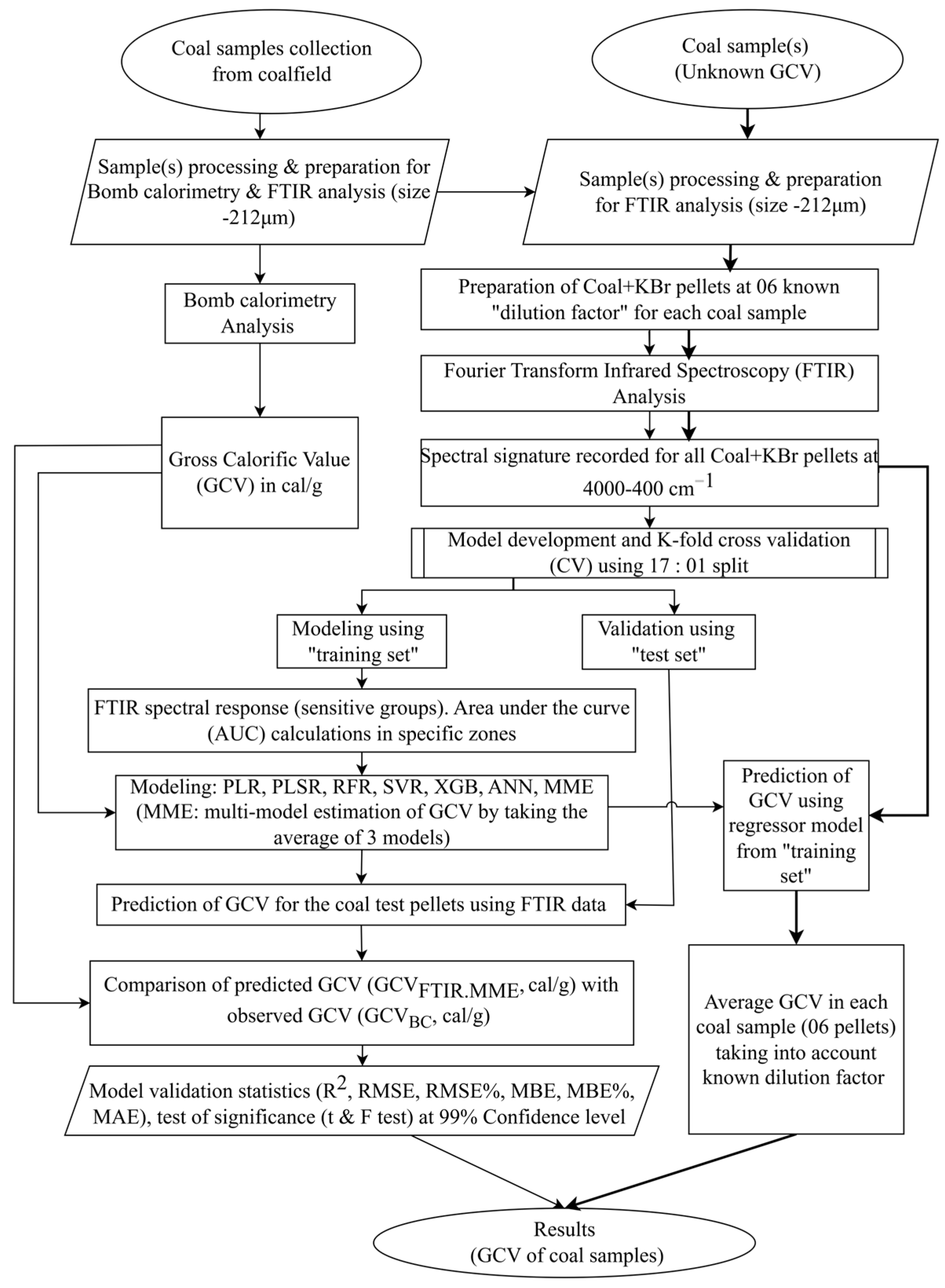
Figure 1. Visual representation of the sequential process for model creation, validation, and prediction of the GCV of coal samples (AUC: area under the curve; PLR: piecewise linear regression; PLSR: partial least squares regression, RFR: random forest regression; SVR: support vector regression; XGB: extreme gradient boosting; ANN: artificial neural network; MME: multi-model estimation).
Applsci 15 12209 g001
Figure 2. Systematic variations in the absorbance observed for analyzed samples at six known concentrations of 0.20%, 0.30%, 0.40%, 0.60%, 1.00%, and 1.4% of coal in coal + KBr pellets, using FTIR spectroscopy in the range 4000 to 400 cm−1 for the sample J_13. P1 to P56 represent the absorbance peak locations related to the different functional group content in coal.
Applsci 15 12209 g002
Figure 3. Distinct absorption bands obtained through FTIR spectroscopy from 600 to 1300 cm−1 for the coal sample J_13.
Applsci 15 12209 g003
Figure 4. Distinct absorption bands obtained through FTIR spectroscopy in the range 1300 to 2300 cm−1 for the coal sample J_13.
Applsci 15 12209 g004
Figure 5. Distinct absorption bands obtained through FTIR spectroscopy in the range 2300 to 4000 cm−1 for the coal sample J_13.
Applsci 15 12209 g005
Figure 6. Scatter plot displaying the correlation between the observed GCV using bomb calorimetry (GCVBC) and model-estimated GCV by FTIR for the coal samples using (a) GCVFTIR.PLR, (b) GCVFTIR.PLSR, (c) GCVFTIR.RFR, (d) GCVFTIR.SVR, (e) GCVFTIR.ANN, and (f) GCVFTIR.XGB methods and the error measures (R2: coefficient of determination; RMSE: root mean square error).
Applsci 15 12209 g006
Figure 7. Scatter plot displaying the correlation between the observed GCV using bomb calorimetry (GCVBC) and multi-model estimated GCV using FTIR (GCVFTIR.MME), along with the error measures (R2: coefficient of determination; RMSE: root mean square error).
Applsci 15 12209 g007
Figure 8. Boxplot comparing the variation in the GCV observed using bomb calorimetry (GCVBC) and estimated values using FTIR combined with machine learning methods (GCVFTIR.PLR, GCVFTIR.PLSR, GCVFTIR.RFR, GCVFTIR.SVR, GCVFTIR.XGB, GCVFTIR.ANN, GCVFTIR.MME).
Applsci 15 12209 g008
Figure 9. Estimated mean bias error (%) distribution in GCV of coal samples using different methods (GCVFTIR.PLR, GCVFTIR.PLSR, GCVFTIR.RFR, GCVFTIR.SVR, GCVFTIR.XGB, GCVFTIR.ANN, GCVFTIR.MME).
Applsci 15 12209 g009
Figure 10. Taylor diagram representation of the performance evaluation of different models (FTIR.PLR, FTIR.PLSR, FTIR.RFR, FTIR.SVR, FTIR.ANN, FTIR.XGB, and FTIR.MME) for GCV estimation in coal.
Applsci 15 12209 g010
Figure 11. Comparison chart depicting observed (GCVBC) and multi-model predicted (GCVFTIR.MME) GCV of coal samples.
Applsci 15 12209 g011
Table 1. The proximate analysis data range and the GCV content observed through bomb calorimetry for the modeled coal samples.
Sample No.Moisture
(wt%)
Ash
(wt%)
Volatile Matter (wt%)Fixed
Carbon (wt%)
GCV (cal/g)
J_0110.1017.8028.3043.805294
J_027.4012.0028.6551.955301
J_039.2012.2026.9551.656021
J_049.8013.0026.9050.305866
J_056.2010.4028.4554.955892
J_066.209.4024.4060.006467
J_0713.805.0027.2054.006771
J_086.7011.4027.2054.706114
J_0911.309.2027.8051.706191
J_108.3013.0027.4551.255691
J_119.3011.2025.4554.056001
J_124.409.5026.8059.306447
J_137.9010.2027.9054.005943
J_145.8011.7032.0550.455665
J_156.208.4031.3054.106317
J_166.1017.5030.2046.204879
J_177.509.8027.9054.806105
J_182.0010.3029.6558.056398
Mean7.67811.22228.03153.0695964.611
Standard Error0.6340.7060.4440.958111.348
Median7.45010.80027.85054.0006011.000
Standard Deviation2.6902.9951.8854.063472.408
Sample Variance7.2348.9693.55416.512223,169.781
Range11.80012.8007.65016.2001892.000
Minimum2.0005.00024.40043.8004879.000
Maximum13.80017.80032.05060.0006771.000
Table 2. The peak (P) assignment details (for peaks 1 to 31) along with the assigned functional group and bond type. The selected wave numbers are based on the available literature [38,66,67,68,69,70,71,72,73].
PeaksMaximumOnsetTerminationFunctional Group & Bond Type
P1671.330664.192674.190Mercaptans and ThioethersC-S
P2694.187674.190718.470
P3755.607725.613769.893Phenyl trisubstituted=C-H bending
P4775.604769.893785.605
P5797.030785.605814.172
P6914.156892.733929.870Epoxides, Benzene ring substitutionC-O-C stretching,
=C-H bending
P7939.867929.870954.153
P81011.2851001.2871021.284Alcohols, Ethers, Esters,
Carboxylic acids,
Anhydrides
C-O stretching
P91032.7111021.2841069.849
P101099.8441069.8491108.415
P111114.1281108.4151138.410
P121164.1211138.4101179.833
P131229.8261179.8331299.816
P141368.3781359.8081374.091Alkanes-CH3
P151378.3771374.0911385.518
P161389.8031385.5181395.517Phenol/Alcohol/Carboxylic acidC-O-H bending
P171401.8771395.5171405.516
P181413.5451405.5161416.943
P191432.6551416.9431436.940
P201441.2251436.9401448.367
P211451.2231448.3671456.937Alkanes and AromaticDeformation vibration of CH3- and
CH2-, vibration
of aromatic hydrocarbon
C=C skeleton
P221462.6501456.9371472.649
P231492.6461486.9331495.503
P241501.2161495.5031505.501
P251512.6431505.5011518.357
P261598.3461585.4901608.344AlkenesC=C
P271611.2011608.3441615.486
P281619.7711615.4861624.056
P291628.3411624.0561634.055
P301638.3401634.0551648.338
P311652.6241648.3381671.192
Table 3. The peak (P) assignment details (for peaks 32 to 56) along with the assigned functional group and bond type. The selected wave numbers are based on the available literature [38,66,67,68,69,70,71,72,73].
PeaksMaximumOnsetTerminationFunctional Group & Bond Type
P321675.4771671.1921682.619Ketones, Aldehydes, Carboxylic acids and EsterC=O
P331691.1901682.6191696.903
P341701.1881696.9031716.900
P351721.1851716.9001732.612
P361736.8971732.6121748.324
P371775.4631769.7501779.748Anhydrides and Acyl halidesC=O
P381785.4621779.7481791.175
P391802.6021791.1751808.316
P402115.4152108.2742119.701Alkynes≡C-H
P412136.8412128.2712142.554
P422162.5522156.8382165.408
P432851.0262821.3032876.737Alkanes (Methyl and methylene symmetric and asymmetric stretching)H-C-H
P442921.0162876.7372948.155
P452958.1542948.1552982.436
P463040.9993008.1473072.423Alkenes, Aromatic,
Carboxylic acid
C=C-H,
O-H
P473100.9913072.4233129.558
P483219.5453205.2623223.831Alkynes, Carboxylic acid≡C-H, O-H
P493233.8293223.8313239.543
P503245.2563239.5433250.970
P513255.2553250.9703263.825
P523275.2523263.8253282.394
P533408.0913289.5363602.349Phenol/Alcohol/Carboxylic
acid
O-H stretching
P543620.5243602.3493646.634
P553652.3423646.6343660.912
P563694.9073660.9123712.334
Table 4. The error measures for GCV prediction determined through PLR, PLSR, RFR, SVR, XGB, ANN, and MME methods.
nPLRPLSRRFRSVRXGBANNMME
R21080.9280.9230.9440.9220.9310.9200.951
RMSE, (cal/g)1086.9197.1696.0417.1196.7227.3655.644
RMSE, %10827.59527.48919.83722.42920.15920.93719.050
MBE, (cal/g)108−0.646−0.302−0.1320.237−0.5750.418−0.336
MBE, %108−1.730−0.6312.6704.8682.2203.1501.420
MAE, (cal/g)1085.4915.6074.1425.0964.4055.3454.053
Table 5. Shows the results of a two-tailed paired t-test to compare the difference in the means of GCV obtained via bomb calorimetry (GCVBC, cal/g) and model-estimated values using FTIR (GCVFTIR.PLR, GCVFTIR.PLSR, GCVFTIR.RFR, GCVFTIR.SVR, GCVFTIR.ANN, GCVFTIR.XGB, GCVFTIR.MME, cal/g) at a 99% confidence level and α = 0.01 for coal samples (μ: mean, σ2: sample variance, n: number of observations, df: degrees of freedom, tstat: calculated t-statistic, tcritical: the critical value for the test, μd: hypothesized difference in mean, p-value: probability distribution for the test, α: significance level).
t-Test: Paired Two Sample for Means, n = 108; df = 107, alpha = 0.01
Pairμσ2tstatp-ValuetcriticalH0: μd = 0
GCVFTIR.PLR38.07648.220.9700.3342.623True
GCVBC38.71653.91
GCVFTIR.PLSR 38.41660.670.4370.6632.623True
GCVBC38.71653.91
GCVFTIR.RFR38.58615.200.2260.8222.623True
GCVBC38.71653.91
GCVFTIR.SVR 38.95599.28−0.3450.7312.623True
GCVBC38.71653.91
GCVFTIR.ANN39.13676.00−0.5880.5582.623True
GCVBC38.71653.91
GCVFTIR.XGB38.14596.160.8880.3772.623True
GCVBC38.71653.91
GCVFTIR.MME38.38611.420.6180.5382.623True
GCVBC38.71653.91
Table 6. Results of a two-tailed F-test to compare the difference in the variance of GCVs obtained via bomb calorimetry (GCVBC, cal/g) and modeling using FTIR (GCVFTIR.PLR, GCVFTIR.PLSR, GCVFTIR.RFR, GCVFTIR.SVR, GCVFTIR.ANN, GCVFTIR.XGB, GCVFTIR.MME, cal/g) at a 99% confidence level and α = 0.01 for coal samples (μ: mean, σ2: sample variance, n: number of observations, df: degrees of freedom, Fstat: calculated F-statistic, CI: confidence interval, σ2o: variance of observed data, σ2p: variance of predicted data, p-value: probability distribution for the test, α: significance level).
F-Test: Two Sample for Equality of Variance, n = 108, df = 107, alpha = 0.01
Pairμσ2Fstatp-ValueCIH0: σ2o = σ2p
GCVFTIR.PLR38.07648.221.0090.9640.611, 1.666True
GCVBC38.71653.91
GCVFTIR.PLSR38.41660.670.9900.9580.599, 1.635True
GCVBC38.71653.91
GCVFTIR.RFR38.58615.201.0630.7530.644, 1.756True
GCVBC38.71653.91
GCVFTIR.SVR38.95599.281.0910.6530.661, 1.802True
GCVBC38.71653.91
GCVFTIR.ANN39.13676.000.9670.8640.586, 1.598True
GCVBC38.71653.91
GCVFTIR.XGB38.14596.161.0970.6330.664, 1.812True
GCVBC38.71653.91
GCVFTIR.MME38.38611.421.0690.7290.648, 1.766True
GCVBC38.71653.91
Table 7. Compares the statistical parameter values found in earlier studies using different methods/equipment/input data/algorithms and the present study, which were used to model and estimate the amount of GCV in coal (PSO-ANN: Particle swarm optimization-artificial neural network, ANFIS: Adaptive neuro-fuzzy inference system, PCA: Principal component analysis, K-ELM: Kernel-based Extreme Learning Machine, WT-MIV-KELM: Wavelet Transform with Mean Impact Value and Kernel-based Extreme Learning Machine; GA: Genetic Algorithm, V-WSP: Variance-Weighted Spectral Preprocessing, MC-UVE: Monte Carlo Uninformative Variable Elimination, GRNN: General regression neural network, RBFNN: Radial basis function neural network, GBRT: Gradient boosted regression trees, GRA: Grey relational analysis CMLM: Committee of machine learning models, SAE: Simple average ensemble, WAE: Weighted average ensemble).
SI.
No
MethodNo. of
Sample
R2RMSE,
MBE
(cal/g)
RMSEP (cal/g)MAE
(cal/g)
Place
(Ref.)
1PLS with NIRS350.95-78.82-China
[79]
2PLS with XRF350.94-93.15-
3PLS with NIRS-XRF (low-level fusion model)350.98-45.40-
4PLSR with NIRS-XRF (mid-level fusion model)350.99-38.20-
5PLS with LIBS160.99-109.4-China
[80]
6Dominant factor-based PLS model with LIBS530.97195.9317.7-China
[18]
7PLS with LIBS450.99-53.7047.80China
[31]
8PLS with NIRS450.99-64.5055.90
9PLS with LIBS & NIRS450.99-45.9040.10
10MLR with Proximate parameters770.72217.3-2.51%India
[2]
11SVR with Proximate parameters770.96174.4-1.58%
12RFR with Proximate parameters770.97143.3-1.38%
13XGBoost with Proximate parameters770.9931.0-0.32%
14MLR with Proximate parameters430.84542.2-5.24%India
[27]
15MLR with Vis-NIR spectra430.92391.7-4.85%
16PSO-ANN with proximate analysis25830.96182.5-0.016Vietnam
[81]
17ANFIS with proximate analysis320.99--2.04%Vietnam
[82]
18ANN with proximate analysis320.99--683.8
19MLR with proximate analysis320.99--3.55%
20SVR with LIBS5500.9-293.800.91%China
[20]
21SVR combined PCA model with LIBS5500.91-203.000.65%
22K-ELM model based on PSO with LIBS280.99-167.20-China
[22]
23WT-MIV-KELM combined with LIBS280.99-146.90-China
[23]
24GA-optimized ANN combined with LIBS270.9664.5-93.10China
[83]
25KELM combined with LIBS280.96-300.60-China
[24]
26V-WSP-KELM with LIBS280.96-237.30-
27PSO-KELM with LIBS280.97-167.20-
28WT-KELM with LIBS280.96-237.30-
29WT-MIV-KELM with LIBS280.98-146.90-
30WT-PSO-KELM with LIBS280.98-116.70-China
[24]
31MC-UVE-KELMwith LIBS280.97-432.50-
32V-WSP-PSO-KELM with LIBS280.99-84.40-
33MVR-Proximate63390.97---USA
[64]
34RF−Proximate63390.97---
35MVR-Ultimate63390.99---
36RF-Ultimate63390.99---
37RF combined with XRF & proximate analysis1810.990.026--China
[17]
38MLR with proximate analysis65200.97205.4-148.10Türkiye
[84]
39MLP with proximate analysis65200.98155.2-112.30
40GRNN with proximate analysis65200.98152.9-109.90
41RBFNN with proximate analysis65200.99148.1-105.10
42MLR with proximate analysis320.99--0.90%Pakistan
[85]
43MLR with proximate analysis85250.98206.6-142.60Türkiye
[86]
44GPR with proximate analysis85250.98183.2-128.40
45MLR with proximate analysis & ultimate analysis85000.9962.1-0.88%Philippines
[87]
46MLR with proximate analysis10180.69---USA
[88]
47ANN with proximate analysis10180.84---
48GRBT with proximate analysis67030.99--110.40USA
[89]
49GRBT with proximate analysis17790.95--124.00
50Decision tree with proximate & ultimate analysis65820.9918,634.8 (MSE) 74.06USA
[76]
51Bagging with proximate & ultimate analysis65821.0011,658.4 (MSE) 56.50
52Random forest with proximate & ultimate analysis65821.0011,320.5 (MSE) 55.83
53Extra trees with proximate & ultimate analysis65821.008905.9 (MSE) 50.72
54Adaptive boosting with proximate & ultimate analysis65820.9863,211.7 (MSE) 149.44
55Gradient boosting with proximate & ultimate analysis65821.0012,491.7
(MSE)
62.11
56XGBoost with proximate & ultimate analysis65821.008168.5 (MSE) 49.56
57SVM with proximate & ultimate analysis33440.9914.689 (MSE) 44.40USA
[78]
58RFR with proximate & ultimate analysis33440.9916.767 (MSE) 46.96
59GBRT with proximate & ultimate analysis33440.9914.522 (MSE) 44.33
60XGB with proximate & ultimate analysis33440.9913.519 (MSE) 42.59
61MLR with proximate analysis500.763805.389-713.67South Africa
[77]
62SVR with proximate analysis500.7342498.329-2403.96
63ANN with proximate analysis500.5642152.719-1560.62
64GRA-CMLM with proximate
analysis
500.909636.525-530.72
65SAE-CMLM with proximate
analysis
500.919679.756-574.19
66WAM-CMLM with proximate
analysis
500.918674.740-569.17
67FTIR with PLR1080.936.919,
−0.646
-5.49India
Present study
[90]
68FTIR with PLSR1080.927.169,
−0.302
-5.61
69FTIR with RFR1080.946.041,
−0.132
-4.14
70FTIR with SVR1080.927.119,
0.237
-5.10
71FTIR with XGB1080.936.722,
−0.575
-4.40
72FTIR with ANN1080.927.365,
0.418
-5.35
73FTIR with MME1080.955.644,
−0.336
-4.05
Disclaimer/Publisher’s Note: The statements, opinions and data contained in all publications are solely those of the individual author(s) and contributor(s) and not of MDPI and/or the editor(s). MDPI and/or the editor(s) disclaim responsibility for any injury to people or property resulting from any ideas, methods, instructions or products referred to in the content.