Abstract
The proposed Adaptive RTR with Quarantine (ARQ) method integrates, within a single evolutionary scheme for continuous optimization, three mature ideas of pbest differential evolution with an archive, success-history parameter adaptation, and restricted tournament replacement (RTR) and extends them with a novel outlier quarantine mechanism. At the heart of ARQ is a combination of the following complementary mechanisms: (1) an event-driven outlier-quarantine loop that triggers on robustly detected tail behavior, (2) a robust center from the best half of the population to which quarantined candidates are gently repaired under feasibility projections, (3) local RTR-based replacement that preserves spatial diversity and avoids premature collapse, (4) archive-guided trial generation that blends current and archived differences while steering toward strong exemplars, and (5) success-history adaptation that self-regulates search from recent successes and reduces manual fine-tuning. Together, these parts sustain focused progress while periodically renewing diversity. Search pressure remains focused yet diversity is steadily replenished through micro-restarts when progress stalls, producing smooth and reliable improvement on noisy or rugged landscapes. In a comprehensive benchmark campaign spanning separable, ill-conditioned, multimodal, hybrid, and composition problems, ARQ was compared against leading state-of-the-art baselines, including top entrants and winners from CEC competitions under identical evaluation budgets and rigorous protocols. Across these settings, ARQ delivered competitive peak results while maintaining favorable average behaviour, thereby narrowing the gap between best and typical outcomes. Overall, this design positions ARQ as a robust choice for practical performance and consistency, providing a dependable tool that can meaningfully strengthen the methodological repertoire of the research community.
1. Introduction
We studied continuous minimization over a rectangulardomain
where is accessed via point wise evaluations (derivatives may be unavailable).
Feasible set and constraints. If constraints are present,
and the task becomes . Box feasibility is enforced by the projection
General constraints can be handled with a penalty functional:
Best-so-far and termination. Given an evaluation budget , an algorithm produces iterates and tracks the best-so-far value
Termination occurs when either or a target quality is reached.
Performance reporting (best and mean). Over R independent runs, let denote the per-run best-so-far value at budget. We report
optionally complemented by average rank across a problem suite.
Following the problem statement, we position our contribution within the main families of continuous optimization. When smoothness and dependable directional information are available, Gradient Descent (GD) remains a natural choice and modern momentum or learning rate schedules extend its reach, although the dependence on differentiability and well behaved curvature can limit robustness on rugged, high dimensional, or strongly multimodal objectives [1]. Newton Raphson can achieve rapid local convergence by exploiting curvature provided stable Hessian information or proper regularization is available [2]. Deterministic derivative free local search such as the Nelder and Mead Simplex Method offers geometry aware progress without gradients and is effective in low to moderate dimensions, yet performance typically degrades as dimensionality and multimodality grow [3]. Stochastic search complements these tools. Monte Carlo simulation legitimizes randomized proposals and statistical summary to probe complex landscapes [4], while simulated annealing regulates uphill acceptance via a temperature schedule to promote principled escapes from local minima [5].
Population based methods expand these ideas with distributed exploration and information sharing. Genetic algorithms model recombination and selection over evolving candidate sets [6]. Particle Swarm Optimization coordinates velocity and position updates to disseminate useful search directions and has inspired stability oriented and diversity oriented refinements, for example CLPSO and modern parallel or optimized variants [7,8,9,10]. Ant Colony Optimization and Artificial Bee Colony bias sampling toward historically promising regions while preserving exploratory motion [11,12,13].
Within this ecosystem, Differential Evolution (DE) has become a central tool for real parameter search due to expressive trial generators and strong empirical performance across heterogeneous test beds [14]. Recent DE progress converges on several effective motifs. Memory based parameter adaptation as in SHADE reduces manual tuning [15]. Population size scheduling as in L-SHADE improves efficiency on diverse suites [16]. Updates in the refined success history as in jSO further stabilize performance under tight evaluation budgets [17]. Multi-population flows, elite regeneration, and adaptive mutation or selection policies add resilience [18,19]. Orthogonal advances include coordinate system learning and eigen informed operators that mitigate ill conditioning and non-separability [20,21], while parallel implementations extend practicality under limited budgets [22]. Targeted DE modifications and implementation guidelines also systematize robust choices in scaling, crossover, and selection [23]. Beyond these families, recent DE advances report improved mutation and parameter control mechanisms [24], and a multi-operator ensemble L-SHADE with restart and local search for single-objective optimization [25], further broadening the toolkit. Additional ensemble/restart-style enhancements likewise expand the L-SHADE lineage [16].
ARQ is motivated by two converging lines: multi-strategy/co-evolutionary DE that strengthens the exploration-exploitation balance across heterogeneous landscapes [26], and robust-statistics principles where trimmed/median location and robust scale safeguard estimates under heavy tails [27]. Adjacent domains (e.g., systems leveraging contextual knowledge to stabilize signals under domain noise) point to the same practical need: preserve a reliable core while injecting measured diversity [28,29]. Within this perspective, we aim for a lightweight yet effective mechanism that turns extremes from destabilizing noise into controlled exploration stimuli.
We propose ARQ, a method aimed at dependable best-so-far progress and competitive mean performance under finite budgets. ARQ integrates pbest DE with an external archive in the JADE or SHADE lineage of archive assisted search and success history adaptation [15,16,17,30]. It applies success history updates of the scale and crossover rates through gain weighted statistics [15,16]. It enforces a neighborhood-aware replacement rule inspired by restricted tournament reasoning to preserve structured diversity [31]. Our contribution is an explicitly triggered tail-quarantine coupled with a trimmed center and micro-restarts, so that stabilization coexists with a steady, low-intensity injection of diversity. The key innovation is an outlier quarantine mechanism. Individuals identified in the extreme tail of the fitness distribution relative to a robust threshold are gently attracted toward a robust population center computed from the better half of the population, with mild perturbation and box projection . When a repaired candidate improves, it is accepted, and the previous one is archived. By trimming distribution tails and re-aligning weak individuals with promising regions, quarantine stabilizes average progress while maintaining the ability to intensify around incumbents. Complementary micro-restarts refresh a small fraction of the worst solutions around the current elite to provide targeted escapes without global resets, while mini-batch updates modulate per-step cost and support scalability [22]. We recommend ARQ in scenarios where one seeks a robust optimizer that consistently achieves strong best-so-far values and reliable mean performance across independent runs. By combining selective attraction, self tuning, neighborhood-aware selection, and principled repair and regeneration, ARQ addresses common failure modes such as premature convergence, tail accumulation of poor individuals, and inefficient restarts, and offers a dependable and broadly applicable tool for continuous optimization.
In relation to recent DE variants, multi-strategy and cooperative/co-evolutionary schemes show that combining complementary operators improves resilience on heterogeneous problems [26]. Applied strands in consumer and industrial settings also report restart- and scheduling-oriented enhancements, such as NSGA-III delay-recovery pipelines and AHMQDE-ACO co-optimization [32,33]. In parallel, micro/partial restarts provide controlled diversity without dissolving the incumbent core [34]. ARQ differs by making tail isolation event-driven (triggered only upon tail inflation), defining a practical robust center as the mean of the top-50%, and systematically coupling quarantine with micro-restarts. The result is a retain-refresh loop that improves convergence consistency with negligible overhead [27,34]. Evidence from business-process control corroborates robustness under operational constraints [35], while e-commerce pricing studies highlight stability in fast-changing demand environments [36]. In transportation analytics, arrival-time prediction pipelines benefit from resilient learning components [37], and distributed privacy-robust learning demonstrates complementary stability in federated settings [38]. Finally, adjacent optimization tasks including trajectory generation and macro-analytics illustrate portability beyond canonical benchmarks [39,40].
ARQ introduces an explicitly event-driven outlier-quarantine loop triggered by tail behavior using a robust cutoff . Flagged samples are quarantined up to a proportion and repaired around a robust center (mean of the best 50%), in tandem with a low-overhead micro-restart. Unlike success-history-only DE variants, this mechanism turns extremes from destabilizing noise into controlled exploration stimuli, yielding a smaller best–mean gap without sacrificing peak performance.
Finally, the remainder of this article is organized as follows: Section 2 details the ARQ method its control flow, parameter-policy with success-history updates, pbest/1/bin trial construction with archive support, neighborhood-aware RTR selection, and the quarantine and micro-restart mechanisms linking the pseudo-code routines to their roles in the overall algorithm. Section 3 describes the experimental setup and real-world benchmarks, the evaluation protocol, and reporting conventions, it then presents the parameter sensitivity analysis (Section 3.3), the complexity analysis with respect to dimension (Section 3.4), and a comparative performance study against strong baselines (Section 3.5). The article concludes with a discussion of findings and implications for robust black-box optimization (Section 4).
2. The ARQ Method
2.1. The ARQ Method with Its Mechanisms
Scope and references to preliminaries. We adopt the continuous minimization setting and feasibility operators introduced in Equations (1)–(4), which define the objective over the box domain, the projection operator onto the box, the optional penalty model for general constraints, and the base distance or normalization metric used throughout.
State and mini-batch size. At iteration t, the algorithm maintains a population of size N and an external archive , together with the incumbent best
A mini-batch size m is used per iteration
Trial generation. For a selected agent , the mutant is formed with a pbest/1/bin scheme with archive support
Then, binomial crossover with index guard produces u
and the candidate is projected to the box, , using the projection already defined in Equation (2).
Success history parameter adaptation. On sampling calls the control rates are drawn around running means and clipped to bounds
Let index successful trials within the current iteration, with gains and normalized weights .
The running means are updated by
and remain unchanged if .
Local replacement via RTR. Let denote the bounds normalized Euclidean distance introduced in the preliminaries, cf. Equation (4). The replacement rule is
Outlier quarantine. Using the fitness values of the current population, compute quartiles and the interquartile range as in the preliminaries. Define the robust threshold
Select a subset with and a robust center c as the mean of the best fifty percent of . For each propose a repair
Targeted micro-restart. Let W be the set containing a fraction w of the worst individuals. For each propose a restart around the incumbent
and accept if , archiving the displaced point. Activation of this mechanism is controlled by the dedicated stagnation trigger.
Termination and reporting. The loop continues while . Upon exit the method returns
and, across R independent runs, we summarize the end-of-budget best-so-far via Equation (6).
Building on the preliminaries and problem conventions, we present ARQ from the overall control flow to its constituent mechanisms. We began with the overall control flow (Algorithm 1 and Figure 1), detailing initialization, the iterative cycle with mini-batch agent updates, success-history parameter adaptation, neighborhood-aware RTR selection, outlier quarantine, and the targeted micro-restart, terminating with the incumbent best. We then analyzed the four core subroutines that implement ARQ’s key building blocks: ParameterPolicy (Algorithm 2 and Figure 2) for sampling and gain-weighted updates of and . TrialGeneration (Algorithm 3 and Figure 3) for pbest/1/bin trial construction with archive support and box projection. SelectionRTR (Algorithm 4 and Figure 4) for local replacement via restricted tournament. PopulationMaintenance (Algorithm 5 and Figure 5), which introduces the outlier-quarantine innovation together with the micro-restart mechanism. We concluded by mapping pseudo-code parameters to implementation controls and highlighting how these components interact to ensure stability and strong performance across diverse search regimes.
| Algorithm 1 ARQ main pseudo-code |
INPUT - f: objective function - : box domain [ℓ1,u1] … [,] - N: population size - T: max evaluations - p: pbest fraction - : fraction updated per step - : mean scale factor - : mean crossover rate - : quarantine threshold coefficient - : repaired outliers fraction - w: worst fraction for micro-restart OUTPUT - , INITIALIZATION - Initialize P with N random solutions in and evaluate f - Set archive and means , - Extract from the best member of P - Set ARQ main pseudo-code 01 While do 02 Compute 03 Draw random subset with 04 Clear , , 05 For each do 06 Obtain F, from ParameterPolicy in sampling mode with input (, ) 07 Obtain y from TrialGeneration with input (x, P, , p, F, , ) 08 Set 09 Set 10 Obtain , from SelectionRTR with input (x, y, , P) 11 If then 12 Append F to 13 Append to 14 Append to 15 Endif 16 If then 17 Set 18 Set 19 Endif 20 Endfor 21 Update (, ) ← via ParameterPolicy. update (, , , ) 22 Apply PopulationMaintenance with input (P, , , , , , w) 23 Endwhile 24 Return , |
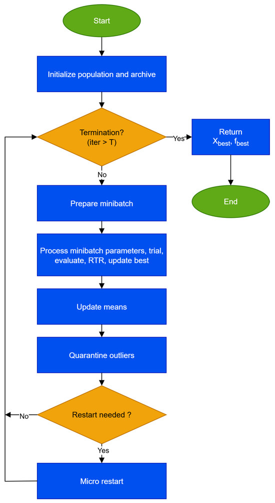
Figure 1.
The ARQ method, an accelerated evolutionary optimization method with success-history adaptation, RTR selection, outlier quarantine, and targeted micro-restart.
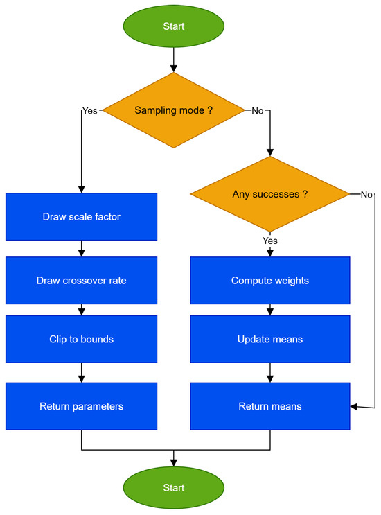
Figure 2.
ParameterPolicy: sampling of control rates and success-history update of running means (fast self-tuning for coherent gains, conservative for scattered ones).

Figure 3.
TrialGeneration: pbest/1/bin trial construction with archive support and box projection (targeted drift toward strong exemplars).
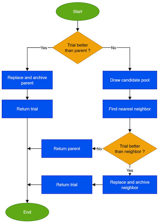
Figure 4.
SelectionRTR: local replacement via restricted tournament with nearest-neighbor check (archiving displaced solutions for future diversity).
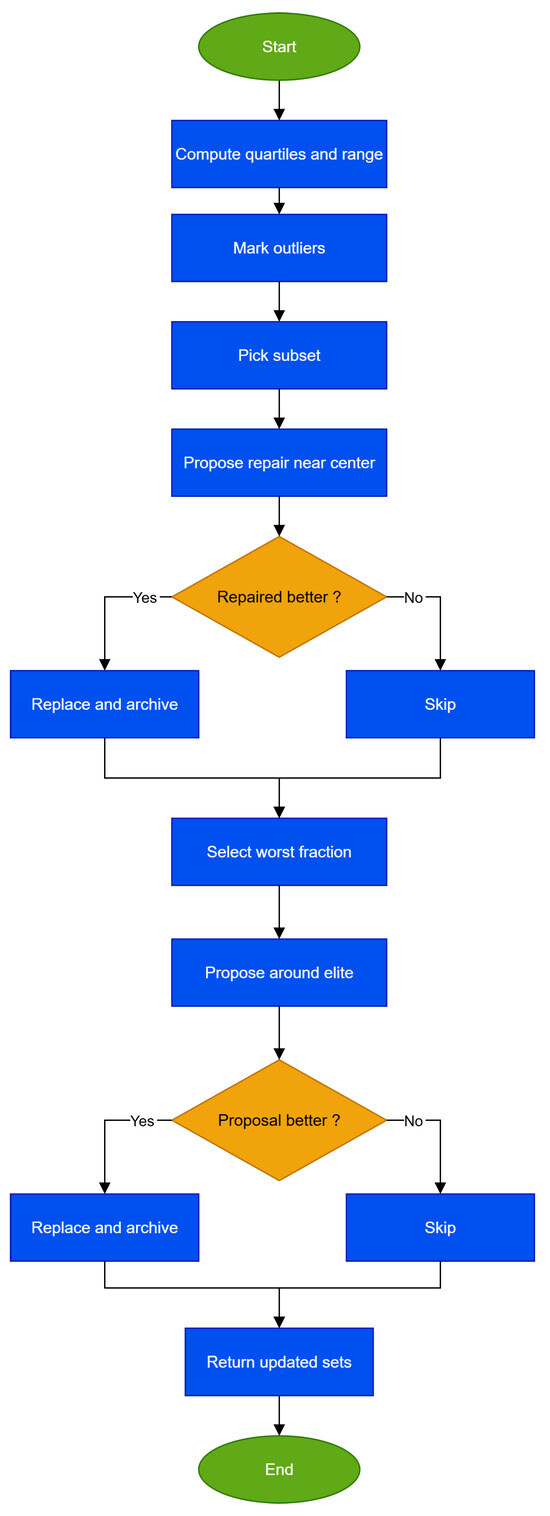
Figure 5.
PopulationMaintenance: outlier quarantine and targeted micro-restart (controlled re-injection/refresh).
Algorithm 1 together with Figure 1 summarizes the control flow of ARQ. The process starts with population and archive initialization and with current means for F and . At each iteration, the termination condition iteration < T is assessed. If budget remains, a mini-batch of agents is selected and a compact improvement cycle is executed. This cycle samples parameters from the success history policy, constructs a pbest/1/bin trial with archive support and box projection, evaluates the trial, and applies neighborhood-aware RTR selection. Successful updates are recorded so that they inform the subsequent mean update. After the mini-batch is processed, the parameter means are updated using gain weighted statistics, outlier quarantine is applied to robustly handle poor solutions, and a targeted micro-restart is performed only when needed around the current incumbent. When the termination condition fails, the algorithm explicitly returns and . This design couples parameter adaptivity, local selection pressure, and controlled population refresh to deliver steady progress while avoiding derailment by outliers or premature convergence.
Algorithm 2 and Figure 2 define the policy of ARQ’s parameter. The routine has two clear modes. In sampling mode, it draws F and around their current means and clips them to preset bounds, supplying the improvement cycle with a controlled blend of exploration and exploitation. In update mode, it gathers the successful trials of the current cycle, forms gains as weights, and computes new means, using a weighted Lehmer mean for F and a weighted arithmetic mean for . This rewards parameters that delivered substantive improvement while damping isolated lucky events. If no successes are recorded, the means are kept unchanged to preserve stability. The result is fast adaptation when profitable directions are coherent and conservative updates when improvements are scattered, aligning the learning pace with the search landscape and avoiding excessive oscillations.
| Algorithm 2 Subroutine ParameterPolicy sampling and update of F, |
INPUT (, , , , , ) OUTPUT 01 If mode = sampling then 02 Draw F from Cauchy centered at and clip to 03 Draw from Normal with mean and clip to 04 Return (F, ) 05 Endif 06 If mode = update then 07 If empty then 08 Return (, ) 10 Endif 11 Normalize weights w from so that sum w = 1 12 Set divided by (sum ) 13 Set sum 14 Return (, ) 15 Endif |
Algorithm 3 and Figure 3 show details of the trial construction pipeline that feeds ARQ’s local improvement. A guide is first drawn from the top fraction of the population so that movement is biased toward promising regions. Two additional guides are then selected, one from the current population and one from either the population or the archive, injecting diverse directions. On these anchors, a pbest/1/bin style mutation is formed that blends an attraction toward the elite guide with a difference of two solutions, striking a balance between exploitation and exploration. Next, component-wise binomial crossover is applied with a guarantee that at least one component originates from the mutant, preventing stagnation. Finally, the candidate is projected back to the box to enforce feasibility, which stabilizes behavior across variable scales. The archive broadens directional cues when progress stalls, and the projection keeps the process constraint compliant without sacrificing trial diversity.
| Algorithm 3 Subroutine TrialGeneration pbest/1/bin with archive and projection |
INPUT (x, P, , p, F, , ) OUTPUT (y) 01 Choose from the top p fraction of P 02 Choose with 03 Choose with and if feasible 04 Compute 05 Sample uniformly from {1,2,…,D} 06 For each coordinate j do 07 If or then 08 set 09 else 10 set 11 Endif 12 Endfor 13 Project u to componentwise to obtain y 14 Return (y) |
The selection routine in Algorithm 4 and Figure 4 implements a restricted tournament to keep replacements local and meaningful. The trial is first tested against its parent and, if superior, it directly replaces the parent while the old solution is archived. Otherwise, a small candidate pool is drawn to maintain computational efficiency. From this pool, the nearest neighbor under bounds normalized distance is identified, making the locality metric scale invariant. The trial is compared only to this neighbor and replaces it if better, with the displaced solution pushed to the archive. If not, the parent is retained. This mechanism concentrates selection pressure where it yields real gains, preserves the spatial structure of the population, mitigates premature convergence, and sustains diversity without incurring substantial overhead.
| Algorithm 4 Subroutine SelectionRTR local replacement with restricted tournament |
INPUT (x, y, , P) OUTPUT (, ) 01 If then 02 Replace x by y in P and archive old x 03 Return (y, ) 04 Endif 05 Draw fixed size pool 06 Find with minimum bounds normalized distance to y 07 If then 08 Replace by y and archive old 09 Return (y, ) 10 Else 11 Return (x, ) 12 Endif |
Unlike the previous routines, Algorithm 5 in Figure 5 explicitly shapes the population. The first phase identifies outliers using the threshold and selects a subset for repair. Each repair proposes a candidate near a robust center computed from the best half of the population and is accepted only if it yields a measurable improvement, with the displaced solution archived. The second phase targets a fraction of the worst individuals for a micro-restart around the current incumbent, using mild, box-scaled perturbations, replacements are again conditional and archived. Together, outlier quarantine and micro-restart prevent the accumulation of toxic points, continually steer the population geometry toward productive regions, and provide a controlled recovery mechanism when progress slows.
| Algorithm 5 Subroutine PopulationMaintenance outlier quarantine and micro-restart |
INPUT (P, , , , , , w) OUTPUT (P, ) 01 Compute , , from fitness values and set 02 Set { with } 03 Compute center c as mean of the best fifty percent of P 04 Choose random subset with 05 For each do 06 Set and project to 07 If then 08 replace and old one 09 Endif 10 Endfor 11 Choose fraction w of the worst individuals of P 12 For each x in that fraction do 13 Set + Normal and project to 14 If then 15 replace and old one 16 Endif 17 Endfor 18 Return (P, ) |
2.2. Design and Parameterization
The outlier quarantine mechanism is introduced to stabilize the search whenever a few very distant samples stretch the solution cloud and weaken the convergence signals. In this situation, standard means and spreads become brittle because the tails dominate. Quarantine temporarily isolates the most extreme portion of the population so that the core can update a reliable location reference and then reinsert the isolated points with a mild, controlled perturbation.
The quarantine proportion is chosen to provide a simple and stable balance between robustness and diversity. We use a small-to-moderate so that only the far tail is removed while the effective population remains intact. In practice, adapts to population size and current dispersion: when the cloud is tight, a very small suffices because outliers are rare, when tails visibly inflate, a slightly larger removes disruptive noise without drying out exploration. This mirrors the logic of a trimmed mean, where clipping a small top slice stabilizes the location estimate.
The perturbation scale determines how strongly quarantined points are reintroduced. We set it relative to the cloud’s current geometry, using robust dispersion measures such as the median absolute deviation or a bounds-normalized per-coordinate standard deviation. When the distribution is compact, a small yields fine local search around the center. When the distribution is scattered or the search is in early phases, a larger helps recapture underrepresented regions. Consequently, with zero-mean always scales to the landscape and avoids unnecessarily large jumps.
We define the robust center as the simple mean of the top half of individuals by fitness because this estimate remains sensitive to improvement and resistant to outliers. The top fifty percent is large enough to reduce random noise and clean enough to exclude low-quality or extreme points. Since the subset is formed by fitness ranking, it concentrates near the promising basin, its plain mean becomes a practical, stable location reference without requiring sophisticated robust estimators.
Synergy with micro-restart is direct and functional. Quarantine suppresses the heavy tail and protects the center estimate from jitter, allowing exploitative operators to move steadily toward the active basin. Micro-restart re-injects small but meaningful diversity near the robust center or along uncertain directions, without dissolving the core. Alternating the two makes the search operate in a retain-refresh cycle: first the tail is smoothed, then the center is updated reliably, and finally exploration resumes with a measured step.
Parameter sensitivity clarifies each effect. Increasing stabilizes references faster but can reduce diversity unless backed by micro-restart. Increasing helps rediscover neighborhoods that would otherwise be missed, but if too large, it weakens local improvement. Using fifty percent to compute the center proved a dependable balance because it keeps statistical efficiency high while remaining outlier-resistant, small deviations around this level do not change qualitative behavior, making it a safe and portable default.
Operationally, the mechanism triggers periodically or when tail inflation is detected via bounds-normalized distances from the center and fitness ranking. Quarantined points are removed, resampled around the center at scale , and reinserted under an acceptance rule that respects the objective while archiving displaced points. In this way we convert extremes from a source of destabilization into controlled exploration stimuli.
The method’s novelty lies in tying three ideas into a light yet effective loop: it makes tail isolation explicit and actionable at the moment it harms estimation, it defines a practical robust center via a simple trimmed average aligned with improvement, and it systematically couples this stabilization with micro-restarts to maintain a steady trickle of fresh variability. The result is a retain-refresh process that improves convergence consistency without heavy adaptation or hyperparameter overhead and that integrates cleanly with existing evolutionary operators. See Figure 6 for the concise flow of quarantine, repair, and reinsertion.
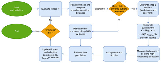
Figure 6.
ARQ flow-detect tail, isolate, resample, and reinsert.
3. Experimental Setup and Benchmark Results
3.1. Setup

Table 1.
ARQ parameters in the pseudo-code.

Table 2.
Parameters of other methods.
Protocol and configurations. Table 2 enumerates the hyper-parameters of all competing methods to enable strict reproducibility under a common budget. Population size is fixed at N = 100. A single termination rule is enforced function evaluations (FEs) and every solver runs under the same budget T. Method-specific controls (e.g., CLPSO comprehensive-learning probability, CMA-ES population and coefficients, EA4Eig JADE-style parameters, mLSHADE_RL and UDE3 [42] success-history memories and pbest ranges, SaDE adaptation schemes) follow the literature and public reference implementations. Complete settings appear in Table 1 and Table 2.
Implementation and environment. All algorithms including the proposed method and baselines were implemented in optimized ANSI C++ and integrated into the open-source OPTIMUS framework [43]. Source code: https://github.com/itsoulos/GLOBALOPTIMUS (accessed on 15 October 2025). Builds used Debian 12.12 with GCC 13.4.
Hardware. Experiments ran on a high-performance node with an AMD Ryzen 9 5950X (16 cores, 32 threads) and 128 GB DDR4 memory, under Debian Linux.
Evaluation protocol. Each benchmark function was executed 30 independent runs with distinct random seeds to capture stochastic variability. With a fixed FE budget, comparisons are made at the same for all solvers.
3.2. Benchmark Functions
Table 3 compiles the real-world optimization problems used in our evaluation. For each case, we report a brief description, the dimensionality and variable types (continuous/mixed-integer), the nature and count of constraints (inequalities/equalities), salient landscape properties (nonconvexity and multi-modality), as well as the evaluation budget and comparison criteria. The set spans, indicatively, mechanical design, energy scheduling, process optimization, and parameter estimation with black-box simulators, ensuring that conclusions extend beyond synthetic test functions. Where applicable, we also note any normalizations or constraint reformulations adopted for fair comparison.

Table 3.
The real world benchmark functions used in the conducted experiments.
3.3. Parameter Sensitivity Analysis of ARQ
Following Lee et al.’s [64] parameter-sensitivity methodology, we constructed a structured analysis to quantify responsiveness to parameter changes and the preservation of reliability across diverse operating regimes.
For the static economic load dispatch one problem, the dominant finding of the sensitivity analysis is that p exhibits by far the largest main effect on mean best (range ≈ 0.937), making it the primary regulator of the exploitation–exploration balance, the trend is clearly decreasing, as increasing p from 0.05 to 0.30 is accompanied by an almost monotonic drop in mean best, with 0.05 emerging as the best setting, indicating that exploitation pressure should remain modest to preserve diversity and avoid population alignment that harms the mean, see Table 4 for the exact main-effect ranges and the per-setting summaries. The main effects and stability ranges are visualized in Figure 7.

Table 4.
Sensitivity analysis of the method parameters for the static economic load dispatch one problem.
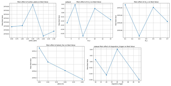
Figure 7.
Sensitivity to selection controllers, main effects, and stability range. Graphical representation of outlier_alpha (), rtr_k (), sh_c (), pbest_frac (p) end stagnation_trigger () for the static economic load dispatch one problem.
The second most influential factor is the success-history memory rate (range ≈ 0.208). Values 0.1 and 0.5 deliver the strongest averages, whereas 0.3 and 0.7 underperform. This matches the expected trade-off: too fast forgetting induces oscillations in F/, while too slow memory anchors prematurely in suboptimal ranges. The data suggest two sweet spots, a more agile setting at 0.1 and a more conservative one at 0.5, implying that problem attributes likely modulate the preferable regime, an adaptive schedule that moves from 0.5 to 0.1 when progress resumes would be reasonable.
The parameter in quarantine/repair shows a moderate main effect (≈0.159), with a peak around 1.5 and only minor differences nearby. Values far below 1.0 or above 2.0 do not improve mean best in this sample. A mid-level aggressiveness for tail definition appears optimal sufficient to trim sporadic failures without crushing diversity supporting the view of quarantine as a noise regulator rather than a hard filter.
The RTR geometry parameter has the smallest main effect in the tested band (≈0.075), with shallow maxima at 5–10 neighbors. This suggests robustness to modest neighborhood changes within the examined range, extremes would likely matter more. A mid-range choice around 5–10 preserves local structure without trapping the population.
The exhibits a small-to-moderate effect (≈0.099), with a best value near 30. Short windows (10–20) do not help mean best, presumably due to premature micro-restarts that cut off promising paths, while very long windows (50) delay exiting genuine stagnation. A trigger around 30 strikes the best balance for the present budget.
Putting this together, the effect ranking is unambiguous: p≫ ≳ > > . A consolidated view of these effects and recommended settings is reported in Table 4. The data-driven recommendation is to fix p at a low level around 0.05, set to either 0.1 or 0.5 depending on algorithmic phase, place near 1.5, choose around 30 generations, and keep in a mid-range of 5–10. While the main-effect signals are clear, confirmatory runs should check for adverse interactions at extreme combinations, especially between p and , and between and .
For dynamic economic dispatch one (ELD1), sensitivity is dominated by p and outlier_alpha with main-effect ranges of ≈0.311 and ≈0.295, whereas , , and play a much smaller role. See Table 5 for the exact main-effect ranges and the per-setting summaries. Unlike the static ELD1, increasing p from 0.05 to 0.30 consistently raises the mean best (peaking at 0.30), indicating that this problem benefits from stronger exploitation, the intertemporal coupling and ramp constraints reward elite-guided moves and reduce the cost of exploratory drift. Higher values (2.0–2.5) further improve the mean best, suggesting that a more permissive tail threshold is advantageous: over-aggressive trimming of outliers can strip away useful diversity needed for smooth cross-period transitions. Changes in are tiny with a slight edge at 0.7, implying that a heavier memory stabilizes F/ adaptation without suppressing peaks, and is marginally better around with negligible differences across the tested band. is essentially neutral with a mild optimum near 30 generations. Overall, the effect ordering is p≳≫≈ > , and the configuration profile emerging for the dynamic case favors a higher p (~0.30), elevated (≈2.0–2.5), slightly slower (~0.7), small (≈3), and around 30 choices that strengthen guided exploitation while avoiding over-sterilization of diversity across time-coupled. The corresponding graphical summary is given in Figure 8.

Table 5.
Sensitivity analysis of the method parameters for the dynamic economic dispatch one problem.
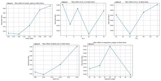
Figure 8.
Sensitivity to selection controllers, main effects, and stability range. Graphical representation of outlier_alpha (), rtr_k (), sh_c (), pbest_frac (p) end stagnation_trigger () for the dynamic economic dispatch one problem.
For Lennard-Jones (13 atoms, 43D) the dominant driver of mean best is (main-effect range ≈ 0.991): heavier success-history memory around 0.7 yields more negative (better) means, improving from −39.33 at 0.1 to −40.32 at 0.7. See Table 6 for the exact main-effect ranges and the per-setting summaries. This indicates that the highly multimodal, deceptive LJ-13 landscape benefits from slower, stabilizing adaptation of F, , which dampens oscillations and sustains coherent progress into deeper energy wells. p shows a moderate effect (≈0.202) with a clear preference for low values, increasing it from 0.05 to 0.30 degrades the mean from −40.02 to −39.82, so restrained exploitation and preserved exploration are essential to avoid alignment around shallow basins. exhibits a modest, favorable trend (≈0.195) as it rises toward 2.0–2.5, a more permissive outlier threshold makes quarantine gentler, which here helps retain useful diversity in challenging basins. and have small effects (≈0.040 and ≈0.014): performance is marginally better near k ≈ 10 and ≈ 50, but differences are minor within the tested band. Overall, LJ-13 favors ≈ 0.7, p ≈ 0.05, ≈ 2.0–2.5, with mid-range and a slightly larger a configuration that promotes steady, directed exploration without overly sterilizing the tails. Notably, the min consistently reaches about −44.33 across settings, suggesting that global-level depths are sporadically discovered regardless, while the recommended choices compress the best–mean gap and systematically improve average quality. See Figure 9 for the main-effect curves.

Table 6.
Sensitivity analysis of the method parameters for problem entitled Lennard-Jones Potential, Atoms 13, Dim: 43.
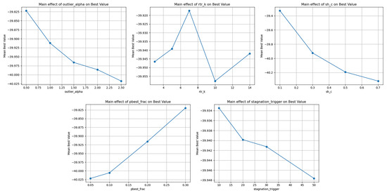
Figure 9.
Sensitivity to selection controllers, main effects, and stability range. Graphical representation of outlier_alpha (), rtr_k (), sh_c (), pbest_frac (p) end stagnation_trigger () for problem of Lennard-Jones Potential, Atoms 13, Dim: 43.
3.4. Analysis of Complexity of ARQ
Below, we present three real-world problems with brief descriptions shell-and-tube heat-exchanger design, a Brayton-type gas-cycle surrogate, and the TANDEM multi-gravity-assist space-trajectory surrogate. In the experiments, we varied only the problem dimension while keeping all modeling and algorithmic settings fixed, so that the observed effects reflect purely the impact of dimensionality. This protocol lets us examine how the proposed optimization method scales as the number of decision variables grows, without confounding changes to constraints, penalties, or hyperparameters. For these measurements, the termination rule was 500 iterations, which proved sufficient to reach the optimal value and thus no additional iterations were required.
3.4.1. Shell-And-Tube Heat Exchanger (Surrogate) [65,66,67]
Vars: . Bounds: m, m, m, , m, .
Heat transfer: , , .
Requirement/penalties: ,
Hydraulics: , , .
3.4.2. Gas Cycle (Brayton-like Surrogate) [68]
Vars: . Bounds: K, K, bar.
3.4.3. Space Trajectory: TANDEM (MGA-1DSM Surrogate) [69,70,71]
Vars (D = 18): . Bounds: (MJD2000 d), , , , , d, .
Compact component forms (surrogate): , , adds DSM shaping terms with , are decreasing functions of leg times, .
Across the three problems, runtime grows smoothly with dimension from 40 to 400 and the trend is very close to linear (Figure 10). Heat exchanger rises from 1.838 s at 40 D to 12.878 s at 400 D, gas cycle from 1.686 s to 11.742 s, and tandem from 2.268 s to 13.116 s. Doubling the dimensionality typically increases runtime by roughly a factor of 1.7–1.9, indicating linear growth with a small fixed overhead at low dimensions. Gas cycle is consistently the fastest, heat exchanger sits in the middle, and Tandem is the slowest, largely due to a higher constant setup cost per evaluation even though its growth rate with dimension is similar to the others. Averaged over the grid, each additional 40 variables adds about 1.1–1.3 s, which remains stable across the range. Overall, the evidence points to an approximately linear time complexity in dimension for the proposed method, with differences between problems attributable mainly to per-evaluation overhead rather than to divergent asymptotic behavior.
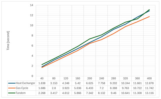
Figure 10.
Runtime vs. dimension (40–400) for ARQ on three real-world problems (500-iteration budget).
3.5. Comparative Performance Analysis of ARQ
Our comparator suite JSO, TRIDENT-DE, UDE3, EA4Eig, mLSHADE_RL, SaDE, CMA-ES, jDE, and CLPSO is a deliberate, sharp, and diverse set that enables fair and generalizable assessment under a common protocol with uniform end-of-budget best-so-far and mean metrics. It blends state-of-the-art DE variants with canonical non-DE references, prioritizing excellence and representativeness (strong CEC and real-world records), so the proposed method is tested against genuinely formidable opponents.
The suite spans the mechanisms that govern the best vs. mean trade-off: aggressive exploitation (pbest/1/bin, current-to-best/1/bin, adaptive F/), diversity preservation (self-adaptation, and mutation ensembles), stagnation handling (restarts and re-initialization), and learning-driven exploration (policy selection). JSO and mLSHADE_RL serve as state-of-the-art DE with robust adaptation/learning and consistent means, TRIDENT-DE is a practitioner-grade baseline known for strong best-so-far, UDE3 probes robustness via ensemble strategies, EA4Eig leverages eigenspace/second-order cues for ill-conditioned landscapes, SaDE tests whether endogenous strategy learning suffices, CMA-ES is the non-DE gold standard learning local geometry via covariance, jDE provides a lightweight self-adaptation lower bound, and CLPSO adds cooperative PSO strength on multimodal/noisy tasks. Together, this mix stresses the proposed method across peak best-so-far, stable mean, and overall robustness, making any observed gains substantive and credible.
Table 7 provides a CEC-style descriptive suite-level summary (best/mean). Statistical tests and significance markers are reported per problem in Table 8, Table 9 and Table 10.

Table 7.
Comparison Based on Best and Mean after FEs.

Table 8.
Detailed Ranking of Algorithms Based on Best after FEs. (1 = green, 2 = blue).

Table 9.
Detailed ranking of algorithms based on mean after FEs. (1 = green, 2 = blue).

Table 10.
Comparison of algorithms and final Ranking. (1 = green, 2 = blue).
Table 7 provides the end-of-budget snapshot, reporting for each real-world task the end-of-budget best-so-far alongside the mean over multiple independent runs. This dual perspective separates peak-attainment from run-to-run consistency, revealing not only who reaches high but also who does so reliably. Within this lens, ARQ exhibits the profile it was designed for: strong best-so-far on rugged or noisy landscapes without sacrificing mean stability. The pattern is mechanistically grounded rather than accidental. Success-history parameter adaptation quickly locks F/CR into profitable ranges, curbing wasteful oscillations that typically inflate variance. Neighborhood-aware RTR replacement focuses selection where it matters while preserving population geometry and diversity, thus avoiding brittle premature convergence. The quarantine mechanism, paired with targeted micro-restarts around the incumbent, trims toxic tails by gently pulling a small fraction of worst individuals toward a robust center and accepting repairs only when they yield genuine improvement. The net effect is a tighter best–mean gap high peaks without bleeding the average.
Reading across problem families reinforces the same message. On geometry-sensitive or ill-conditioned settings, where eigenspace-aware or covariance-adapting methods traditionally shine, ARQ maintains a competitive mean precisely because tail control suppresses rare catastrophic runs that would otherwise drag the average down. On energy and network planning tasks, micro-restarts provide inexpensive, targeted escapes from stagnation that accumulate into steady gains in both best and mean. On classic multimodal benchmarks, the combination of pbest/1/bin with an archive and success-history keeps exploration directed late into the budget, which shows up as robust best-so-far without a collapse in mean.
The deltas between best and mean act as a health indicator of the performance distribution. Where ARQ ties or narrowly trails specialized competitors in best, it often compensates with a superior mean, signaling run-level resilience. Where it attains the top best, the mean remains stable, indicating not a solitary spike but a cohesive cloud of good solutions around it. Because all solvers run under a harmonized protocol, identical budgets, and multiple independent trials, this advantage cannot be dismissed as a tuning artifact. Table 7 therefore suggests that ARQ achieves the hard balance between peak best-so-far and preserved mean through a cohesive TRIDENT-DE: gain-weighted parameter learning, neighborhood-sensitive replacement that protects geometry and diversity, and tail control via quarantine and micro-restarts. This sets the stage for the rankings that follow, in which superior peaks are not purchased at the expense of stability.
Table 8 converts the raw outcomes of Table 7 into per-problem ranks and aggregate indicators, making it explicit whether a solver wins consistently or only sporadically. The pattern for ARQ is a high density of top 1/2 finishes across a broad portion of the suite, accompanied by a low average rank and a tight spread. This indicates breadth and stability rather than a handful of outlier peaks.
The juxtaposition of best-rank and mean-rank indicates a balanced profile. When ARQ achieves a top end-of-budget best-so-far, it does not incur a collapse in mean-rank, this suggests that tail control and micro-restarts keep the population concentrated around the most promising basin. Conversely, in cases where highly specialized competitors hold a slight edge in best-rank, ARQ often compensates with a superior mean-rank, evidencing run-level resilience and an ability to avoid degenerative trajectories.
The geography of ranks across problem families reinforces this reading. On ill-conditioned or geometry-sensitive tasks, where methods that learn search-space geometry traditionally excel, ARQ remains near the front with limited variance, consistent with neighborhood-aware replacement preserving structure and diversity. On multimodal landscapes, where occasional spectacular hits can inflate best-rank while harming mean behavior, Table 8 shows a small gap between ARQ’s two ranking columns, in line with directed exploration sustained late into the budget. On energy and network design applications, micro-restarts around the incumbent accumulate incremental gains that lower average rank and increase the frequency of top-2 placements.
Head-to-head comparisons against recognized state-of-the-art references highlight that ARQ competes not only within the DE family but also against non-DE geometry-learning approaches, reducing the likelihood that its advantage is a tuning artifact. The overall rank and the accompanying aggregates distill this behavior into a single index, yielding clear evidence of generalizability: ARQ does not win only here and there, but stays consistently near the top across heterogeneous classes of problems.
In Figure 11, we report one-sided paired Wilcoxon signed-rank tests (hypothesis ARQ < Other) across all datasets, with Benjamini–Hochberg (FDR) adjustment. ARQ achieves lower ranks on average and is significantly better than most competitors after FDR correction specifically, ARQ vs. UDE3, mLSHADE_RL, CMA-ES, EA4Eig, SaDE, jDE, and CLPSO are significant, whereas ARQ vs. JSO and ARQ vs. TRIDENT-DE remain non-significant. Overall, ARQ shows consistent improvements in rank relative to most alternatives, while being statistically indistinguishable from the two strongest baselines (JSO and TRIDENT-DE). Consistent with the per-problem best outcomes, Figure 12 presents the aggregate mean ranking, condensing averages. Consistent with the per-problem best outcomes, Figure 13 highlights ARQ’s frequent top-tier placements.
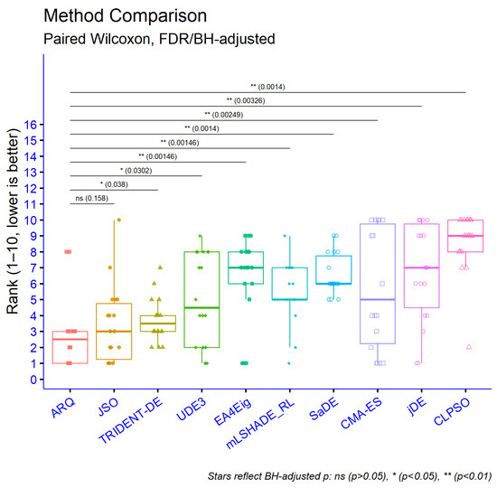
Figure 11.
Statistical comparison of optimization methods by best-so-far over 30 runs (evaluation budget 150,000 FEs).
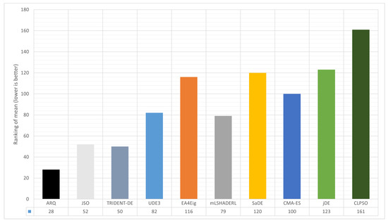
Figure 12.
Aggregate mean ranking across ten algorithms.
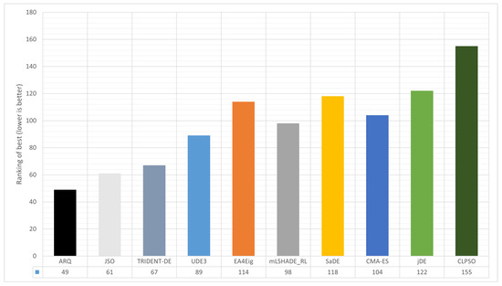
Figure 13.
Aggregate best ranking across ten algorithms.
Table 9 acts as a distillation of the evidence: per-problem ranks are aggregated into global indicators that capture overall behavior. ARQ’s position on these summary measures reflects a solver that excels not by isolated flashes, but by maintaining persistently strong showings across the board. Totals and average ranks remain low, with a tight dispersion around the central tendency, in practice, this means frequent proximity to the top with limited variability from task to task.
The alignment between summary metrics derived from best and from mean confirms the balance observed previously. When ARQ signals strength at the end-of-budget best-so-far, the mean-based summary does not erode, indicating that the cloud of solutions is cohesive rather than driven by rare spikes. Even where narrowly specialized competitors gain a local edge, the cumulative ranking over the whole suite shifts the advantage back to ARQ, because small, steady improvements add up.
What emerges from Table 9 is not merely many first places, but a combination of high top-2 frequency with a scarcity of poor outcomes. ARQ exhibits a compact performance profile: the tails of weak runs are curtailed while strong results appear repeatedly, not accidentally. This distributional shape explains why the global indicators favor the method. In practical terms, Table 9 certifies that the proposed approach preserves a competitive margin as problem geometry, conditioning, and multimodality vary. Consistency across these shifts is precisely what converts scattered victories into an overall lead.
In Figure 14, ARQ secures a clearly lower average rank and leaves most rivals behind even after multiple-comparison control. The strongest pairwise gains are against UDE3, mLSHADE_RL, CMA-ES, EA4Eig, SaDE, jDE, and CLPSO, whereas its gaps to JSO and TRIDENT-DE do not rise to statistical significance. In short, ARQ consistently ranks better than the bulk of competing methods while being on par with the two top baselines (JSO, TRIDENT-DE). Figure 12 presents the aggregate mean ranking, condensing averages. Figure 13 highlights ARQ’s frequent top-tier placements.e performance into a single comparative view.
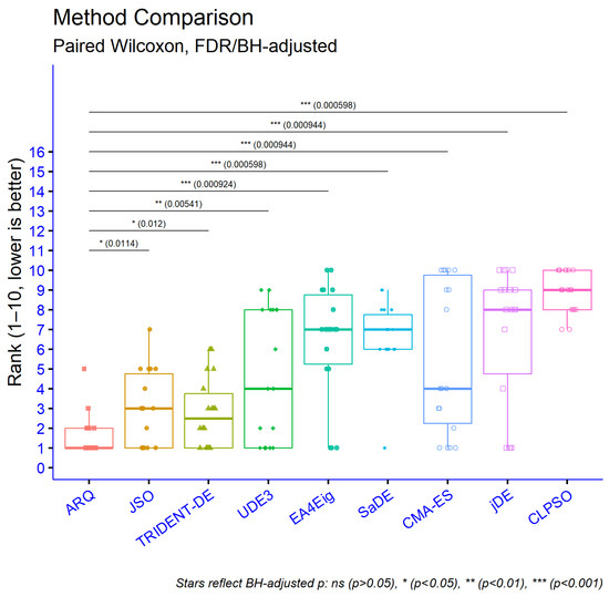
Figure 14.
Statistical comparison of optimization methods by mean best-so-far over 30 runs (evaluation budget 150,000 FEs).
Table 10 consolidates the picture established earlier: ARQ attains the lowest total rank on both best and mean 49 and 28, respectively for a combined sum of 77, corresponding to an average rank of 2.139. The next best competitor sits noticeably higher (e.g., JSO: 61 + 52 = 113), and others trail further behind, indicating that ARQ’s advantage stems from consistent top placements across the suite rather than isolated spikes. This result is aligned with the harmonized experimental protocol and the carefully matched competitor settings, which lends credibility to the comparison.
The pattern strong totals in best without erosion in mean is consistent with ARQ’s design. Success-history parameter adaptation stabilizes profitable ranges for F and CR early on, neighborhood-aware RTR preserves structure and diversity via local replacement, and the outlier-quarantine mechanism with targeted micro-restarts trims tail failures. Together, these components compress the gap between peak and average performance, a behavior visible in Table 7 and now distilled by the aggregates in Table 10. In practical terms, ARQ achieves high end-of-budget best-so-far without paying for it with a degraded mean, and this translates directly into low overall ranks.
In Figure 15, we compare ten algorithms over 36 problems using average ranks and assess pairwise differences with the Nemenyi test (). The pattern is clear: ARQ attains the best mean rank and is significantly better than UDE3 (), mLSHADE_RL (), CMA-ES (), EA4Eig (), SaDE (), jDE () and CLPSO (), while its differences with JSO (p ≈ 0.93) and TRIDENT-DE () are not significant. JSO and TRIDENT-DE form the next tier: each is significantly better than CMA-ES ( and , respectively) and markedly better than EA4Eig, SaDE, jDE and CLPSO ), but neither differs from ARQ and they do not differ from each other. The mid-ranked group (UDE3, mLSHADE_RL, CMA-ES) shows mostly non-significant pairwise differences, except that CMA-ES is worse than JSO and TRIDENT-DE as noted above. CLPSO is the worst on average and is significantly worse than ARQ, JSO, TRIDENT-DE, UDE3, mLSHADE_RL, CMA-ES and EA4Eig (), but its gaps to SaDE and jDE are not significant at ( and , respectively). Overall, the global ranking differences are strong, with ARQ leading; JSO and TRIDENT-DE are competitive with ARQ, whereas the remaining methods particularly CMA-ES, EA4Eig, SaDE, jDE and CLPSO trail with multiple significant deficits. Figure 16 reports the combined (best + mean) ranking as a single bar chart, offering a holistic view that aligns with the consolidated statistics in Table 10.
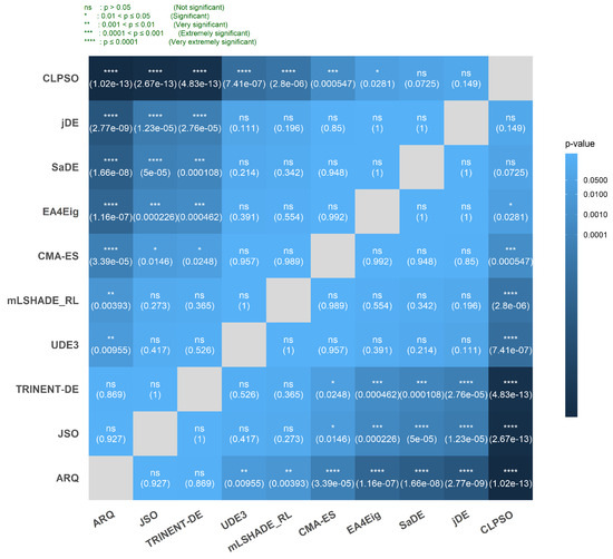
Figure 15.
Per-method significance heatmap: ARQ vs. competitors (Wilcoxon signed-rank with Holm correction; effect direction encoded by color).
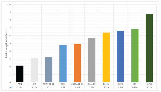
Figure 16.
Total ranking combining best and mean across ten algorithms.
An additional point is breadth. The per-problem rankings show competitiveness on geometry-sensitive and ill-conditioned landscapes as well as on multimodal and application-driven tasks in energy and network planning, where incremental gains must accumulate reliably. That ARQ remains first overall despite strong specialists CMA-ES in highly correlated settings or JSO/mLSHADE_RL for mean stability suggests that its mechanisms address the common failure modes of stochastic optimization: premature convergence, accumulation of weak individuals in the tails, and coarse-grained restarts. Given the aligned configurations and transparent implementation, the evidence supports a substantive rather than accidental advantage.
4. Conclusions
This study demonstrates that ARQ achieves the intended balance between strong end-of-budget best-so-far and preserved mean performance under a strictly harmonized protocol and a demanding comparator suite. Population size, evaluation budget, and opponent configurations are aligned to minimize confounders and ensure reproducibility.
The comparator set spans state-of-the-art DE variants and canonical non-DE references with complementary strengths self-adaptation, policy learning, eigenspace/second-order cues, and swarm strategies so conclusions are not confined to a single operator family.
In terms of metrics, Table 10 consolidates ARQ’s advantage: it attains the lowest total rank on best and mean (49 and 28, sum 77, average rank 2.139), with the next best solver noticeably higher, indicating breadth rather than isolated spikes.
Table 9 clarifies the distributional shape behind this outcome a compact profile with frequent top placements and few poor runs while Table 8 shows that peaks do not come at the expense of stability, when ARQ narrowly trails in best, it typically compensates with a superior mean.
Mechanistically, the behavior is consistent with ARQ’s cohesive design. Success-history adaptation quickly locks F/ into profitable ranges, neighborhood-aware RTR preserves geometry and diversity while channeling selection pressure locally, outlier quarantine together with targeted micro-restarts trims tail failures and provides controlled recovery when progress stalls. The net effect is a persistently small best–mean gap that appears at the per-problem level and crystallizes in the aggregate ranks.
In the present study we targeted , , , p, and because they map to ARQ’s four core mechanisms (TrialGeneration, ParameterPolicy, SelectionRTR, and PopulationMaintenance with micro-restart) and they exhibit material, measured main effects in Table 4, Table 5 and Table 6 and Figure 7, Figure 8 and Figure 9, thereby covering the decisive levers for mean and best performance as well as stability. In a forthcoming updated release of ARQ, we will also include principled techniques for parameter setting such as fractional–factorial screening and response–surface tuning together with automated controllers such as success-history adaptation and auto-tuning of the restart trigger, so that recommended defaults emerge from data rather than manual selection.
The contribution thus lies not in a single trick but in a principled combination of mature ideas that interact constructively, explaining why ARQ competes strongly against both DE and non-DE geometry-learning methods on ill-conditioned or correlated landscapes.
Validity is reinforced by three factors. First, strict resource alignment reduces the chance of artificial gains.
Second, the heterogeneous set of real-world tasks from physico-chemical potentials and code design to energy/network planning and interplanetary trajectories supports generalization.
Third, the explicit exposition of subroutines and controls makes the link between design choices and observed behavior transparent.
There are limitations. Results are reported for a evaluation budget and a specific population size, while parameter sensitivity follows a structured methodology, a deeper map of the interactions among , , and w, together with the micro-restart trigger, would clarify edge-case trade-offs.
Moreover, although the benchmark suite is diverse, scenarios with time-varying noise or large-scale mixed-integer constraints remain under-explored.
These observations motivate several research avenues. Adaptive control of quarantine intensity via data-driven tuning of and the repair fraction , informed by tail statistics and diversity indices, could balance tail-cutting with exploration more finely.
Policy-learning to orchestrate the handover between RTR replacement and restart regimes may further compress the best–mean gap on stagnation-prone landscapes. Geometry-aware differences and archive schemes that periodically estimate principal directions could improve progress on highly correlated objectives without sacrificing DE’s simplicity. Asynchronous mini-batch updates and population-fraction scheduling deserve attention for better hardware utilization. Finally, coupling ARQ with active resampling on noisy objectives, and profiling per-subroutine complexity relative to f-call costs, would sharpen guidance for tight-budget or expensive-evaluation settings.
What distinguishes ARQ. The tail-quarantine loop (with for a robust threshold and for controlled repair intensity), coupled with the robust center and micro-restarts, acts as a diversity-stabilizing mechanism that cooperates with success-history parameter adaptation. In practice, this delivers consistent mean performance together with strong best results, avoiding the large volatility often observed with adaptation-only DE settings.
Overall, the evidence supports a clear conclusion: a cohesive blend of parameter self-adaptation, neighborhood-aware selection, tail control, and targeted regeneration can deliver top-tier best-so-far while keeping the mean stable. Given resource alignment and implementation transparency, ARQ’s advantage appears substantive and practically relevant, providing a dependable optimization tool for heterogeneous, challenging real-world landscapes.
Author Contributions
Conceptualization, I.G.T.; Software, V.C.; Validation, A.M.G. and D.T.; Visualization, A.M.G. All authors have read and agreed to the published version of the manuscript.
Funding
This research has been financed by the European Union: Next Generation EU through the Program Greece 2.0 National Recovery and Resilience Plan, under the call RESEARCH-CREATE-INNOVATE, project name “iCREW: Intelligent small craft simulator for advanced crew training using Virtual Reality techniques” (project code: TAEDK-06195).
Institutional Review Board Statement
Not applicable.
Informed Consent Statement
Not applicable.
Data Availability Statement
The original contributions presented in this study are included in the article. Further inquiries can be directed to the corresponding author.
Conflicts of Interest
The authors declare no conflicts of interest.
References
- Tapkin, A. A Comprehensive Overview of Gradient Descent and its Optimization Algorithms. Int. Adv. Res. J. Sci. Eng. Technol. 2023, 10, 37–45. [Google Scholar] [CrossRef]
- Cawade, S.; Kudtarkar, A.; Sawant, S.; Wadekar, H. The Newton-Raphson Method: A Detailed Analysis. Int. J. Res. Appl. Sci. Eng. (IJRASET) 2024, 12, 729–734. [Google Scholar] [CrossRef]
- Nelder, J.A.; Mead, R. A simplex method for function minimization. Comput. J. 1965, 7, 308–313. [Google Scholar] [CrossRef]
- Bonate, P.L. A Brief Introduction to Monte Carlo Simulation. Clin. Pharmacokinet. 2001, 40, 15–22. [Google Scholar] [CrossRef] [PubMed]
- Eglese, R.W. Simulated annealing: A tool for operational research. Eur. J. Oper. Res. 1990, 46, 271–281. [Google Scholar] [CrossRef]
- Holland, J.H. Adaptation in Natural and Artificial Systems; University of Michigan Press: Ann Arbor, MI, USA, 1975. [Google Scholar]
- Kennedy, J.; Eberhart, R. Particle swarm optimization. In Proceedings of the ICNN’95-International Conference on Neural Networks, Perth, WA, Australia, 27 November–1 December 1995; Volume 4, pp. 1942–1948. [Google Scholar] [CrossRef]
- Liang, J.J.; Qin, A.K.; Suganthan, P.N.; Baskar, S. Comprehensive learning particle swarm optimizer for global optimization of multimodal functions. IEEE Trans. Evol. Comput. 2006, 10, 281–295. [Google Scholar] [CrossRef]
- Charilogis, V.; Tsoulos, I.G. Toward an Ideal Particle Swarm Optimizer for Multidimensional Functions. Information 2022, 13, 217. [Google Scholar] [CrossRef]
- Charilogis, V.; Tsoulos, I.G.; Tzallas, A. An Improved Parallel Particle Swarm Optimization. SN Comput. Sci. 2023, 4, 766. [Google Scholar] [CrossRef]
- Dorigo, M.; Di Caro, G. Ant Colony Optimization. In Proceedings of the 1999 Congress on Evolutionary Computation-CEC99, Washington, DC, USA, 6–9 July 1999; Volume 2, pp. 1470–1477. [Google Scholar] [CrossRef]
- Karaboga, D. An idea based on honey bee swarm for numerical optimization: Artificial bee colony (ABC) algorithm. J. Glob. Optim. 2005, 39, 459–471. [Google Scholar] [CrossRef]
- Kyrou, G.; Charilogis, V.; Tsoulos, I.G. Improving the Giant-Armadillo Optimization Method. Analytics 2024, 3, 225–240. [Google Scholar] [CrossRef]
- Pant, M.; Zaheer, H.; Garcia-Hernandez, L.; Abraham, A. Differential Evolution: A review of more than two decades of research. Eng. Appl. Artif. Intell. 2020, 90, 103479. [Google Scholar] [CrossRef]
- Tanabe, R.; Fukunaga, A. Success-History Based Parameter Adaptation for Differential Evolution (SHADE). In Proceedings of the 2013 IEEE Congress on Evolutionary Computation (CEC), Cancún, Mexico, 20–23 June 2013; pp. 71–78. [Google Scholar] [CrossRef]
- Tanabe, R.; Fukunaga, A.S. Improving the search performance of SHADE using linear population size reduction (L-SHADE). In Proceedings of the 2014 IEEE Congress on Evolutionary Computation (CEC), Beijing, China, 6–11 July 2014; pp. 1658–1665. [Google Scholar] [CrossRef]
- Brest, J.; Maučec, M.S.; Boskovic, B. jSO: An advanced differential evolution algorithm using success-history and linear population size reduction. In Proceedings of the 2017 IEEE Congress on Evolutionary Computation (CEC), Donostia/San Sebastián, Spain, 5–8 June 2017; pp. 1995–2002. [Google Scholar] [CrossRef]
- Cao, Y.; Luan, J. A novel differential evolution algorithm with multi-population and elites regeneration. PLoS ONE 2024, 19, e0302207. [Google Scholar] [CrossRef]
- Sun, Y.; Wu, Y.; Liu, Z. An improved differential evolution with adaptive population allocation and mutation selection. Expert Syst. Appl. 2024, 258, 125130. [Google Scholar] [CrossRef]
- Hansen, N.; Ostermeier, A. Completely derandomized self-adaptation in evolution strategies. Evol. Comput. 2001, 9, 159–195. [Google Scholar] [CrossRef]
- Bujok, P.; Kolenovský, P. Eigen crossover in cooperative model of evolutionary algorithms applied to CEC 2022 single objective numerical optimisation. In Proceedings of the 2022 IEEE Congress on Evolutionary Computation (CEC), Padua, Italy, 18–23 July 2022; pp. 1–8. [Google Scholar] [CrossRef]
- Charilogis, V.; Tsoulos, I.G. Parallel Implementation of the Differential Evolution Method. Analytics 2023, 2, 17–30. [Google Scholar] [CrossRef]
- Charilogis, V.; Tsoulos, I.G.; Tzallas, A.; Karvounis, E. Modifications for the Differential Evolution Algorithm. Symmetry 2022, 14, 447. [Google Scholar] [CrossRef]
- Deng, W.; Shang, S.; Cai, X.; Zhao, H.; Song, Y.; Xu, J. An improved differential evolution algorithm and its application in optimization problem. Soft Comput. 2021, 25, 5277–5298. [Google Scholar] [CrossRef]
- Chauhan, D.; Trivedi, A.; Shivani. A Multi-operator Ensemble LSHADE with Restart and Local Search Mechanisms for Single-objective Optimization. arXiv 2024, arXiv:2409.15994. [Google Scholar] [CrossRef]
- Deng, W.; Shang, S.; Zhang, L.; Lin, Y.; Huang, C.; Zhao, H.; Ran, X.; Zhou, X.; Chen, H. Multi-strategy quantum differential evolution algorithm with cooperative co-evolution and hybrid search for capacitated vehicle routing. IEEE Trans. Intell. Transp. Syst. 2025, 26, 18460–18470. [Google Scholar] [CrossRef]
- Huber, P.J.; Ronchetti, E.M. Robust Statistics, 2nd ed.; Wiley: Hoboken, NJ, USA, 2009. [Google Scholar] [CrossRef]
- Guo, D.; Zhang, S.; Yang, B.; Lin, Y.; Li, J. Exploring contextual knowledge-enhanced speech recognition in air traffic control communication: A comparative study. IEEE Trans. Neural Netw. Learn. Syst. 2025, 36, 16085–16099. [Google Scholar] [CrossRef] [PubMed]
- Guo, D.; Zhang, S.; Lin, Y. Multi-modal intelligent situation awareness in real-time air traffic control: Control intent understanding and flight trajectory prediction. Chin. J. Aeronaut. 2024, 37, 103376. [Google Scholar] [CrossRef]
- Zhang, J.; Sanderson, A.C. JADE: Adaptive differential evolution with optional external archive. IEEE Trans. Evol. Comput. 2009, 13, 945–958. [Google Scholar] [CrossRef]
- Lima, C.F.; Lobo, F.G.; Goldberg, D.E. Investigating restricted tournament replacement in ECGA for stationary and non-stationary optimization. In Proceedings of the 10th Annual Conference on Genetic and Evolutionary Computation (GECCO ’08), Atlanta, GA, USA, 12–16 July 2008; pp. 1–8. [Google Scholar] [CrossRef]
- Deng, W.; Li, X.; Zhao, H.; Xu, J. PSO-K-means clustering-based NSGA-III for delay recovery. IEEE Trans. Consum. Electron. 2025; Advance online publication. [Google Scholar] [CrossRef]
- Zhao, H.; Deng, W.; Lin, Y. Joint optimization scheduling using AHMQDE-ACO for key resources in smart operations. IEEE Trans. Consum. Electron. 2025; Advance online publication. [Google Scholar] [CrossRef]
- Shen, Y.; Zhang, N.; Wang, Z.; Wang, X. Dual-performance multi-subpopulation adaptive restart differential evolution (DPR-MGDE). Symmetry 2025, 17, 223. [Google Scholar] [CrossRef]
- Horita, H. Optimizing runtime business processes with fair workload distribution. J. Compr. Bus. Adm. Res. 2025, 2, 162–173. [Google Scholar] [CrossRef]
- Sun, J.; Wang, Z.; Qiao, Z.; Li, X. Dynamic pricing model for e-commerce products based on DDQN. J. Compr. Bus. Adm. Res. 2024, 1, 171–178. [Google Scholar] [CrossRef]
- Deng, W.; Li, K.; Zhao, H. A flight arrival time prediction method based on cluster clustering-based modular with deep neural network. IEEE Trans. Intell. Transp. Syst. 2024, 25, 6238–6247. [Google Scholar] [CrossRef]
- Li, X.; Zhao, H.; Xu, J.; Deng, W. APDPFL: Anti-poisoning attack decentralized privacy-enhanced federated learning scheme for flight operation data sharing. IEEE Trans. Wirel. Commun. 2024, 23, 19098–19109. [Google Scholar] [CrossRef]
- Ran, X.; Suyaroj, N.; Tepsan, W.; Lei, M.; Ma, H.; Zhou, X.; Deng, W. A novel fuzzy system-based genetic algorithm for trajectory segment generation in urban GPS. J. Adv. Res. 2025; in press. [Google Scholar] [CrossRef]
- Lopatin, A. Intelligent system of estimation of total factor productivity (TFP) and investment efficiency in the economy with external technology gaps. J. Compr. Bus. Adm. Res. 2023, 1, 160–170. [Google Scholar] [CrossRef]
- Charilogis, V.; Tsoulos, I.G.; Gianni, A.M. TRIDENT-DE: Triple-Operator Differential Evolution with Adaptive Restarts and Greedy Refinement. Future Internet 2025, 17, 488. [Google Scholar] [CrossRef]
- Dehghani, M.; Trojovská, E.; Trojovský, P.; Malik, O.P. OOBO: A new metaheuristic algorithm for solving optimization problems. Biomimetics 2023, 8, 468. [Google Scholar] [CrossRef] [PubMed]
- Tsoulos, I.G.; Charilogis, V.; Kyrou, G.; Stavrou, V.N.; Tzallas, A. OPTIMUS: A Multidimensional Global Optimization Package. J. Open Source Softw. 2025, 10, 7584. [Google Scholar] [CrossRef]
- Das, S.; Abraham, A.; Chakraborty, U.K.; Konar, A. Differential evolution using a neighborhood-based mutation operator. IEEE Trans. Evol. Comput. 2009, 13, 526–553. [Google Scholar] [CrossRef]
- Kluabwang, J.; Thomthong, T. Solving parameter identification of frequency modulation sounds problem by modified adaptive tabu search under management agent. Procedia Eng. 2012, 31, 1006–1011. [Google Scholar] [CrossRef][Green Version]
- Ahandan, M.A.; Alavi-Rad, H.; Jafari, N. Frequency modulation sound parameter identification using shuffled particle swarm optimization. Int. J. Appl. Evol. Comput. 2013, 4, 1–15. [Google Scholar] [CrossRef][Green Version]
- Lennard-Jones, J.E. On the determination of molecular fields. Proc. R. Soc. A 1924, 106, 463–477. [Google Scholar] [CrossRef]
- Hofer, E.P. Optimization of bifunctional catalysts in tubular reactors. J. Optim. Theory Appl. 1976, 18, 379–393. [Google Scholar] [CrossRef]
- Luus, R.; Dittrich, J.; Keil, F.J. Multiplicity of solutions in the optimization of a bifunctional catalyst blend in a tubular reactor. Can. J. Chem. Eng. 1992, 70, 780–785. [Google Scholar] [CrossRef]
- Luus, R.; Bojkov, B. Global optimization of the bifunctional catalyst problem. Can. J. Chem. Eng. 1994, 72, 160–163. [Google Scholar] [CrossRef]
- Javinsky, M.A.; Kadlec, R.H. Optimal control of a continuous flow stirred tank chemical reactor. AIChE J. 1970, 16, 916–924. [Google Scholar] [CrossRef][Green Version]
- Soukkou, A.; Khellaf, A.; Leulmi, S.; Boudeghdegh, K. Optimal control of a CSTR process. Braz. J. Chem. Eng. 2008, 25, 799–812. [Google Scholar] [CrossRef][Green Version]
- Pinheiro, C.I.C.; de Souza, M.B., Jr.; Lima, E.L. Model predictive control of reactor temperature in a CSTR with constraints. Comput. Chem. Eng. 1999, 23, 1553–1563. [Google Scholar] [CrossRef]
- Tersoff, J. New empirical approach for the structure and energy of covalent systems. Phys. Rev. B 1988, 37, 6991–7000. [Google Scholar] [CrossRef] [PubMed]
- Tersoff, J. Modeling solid-state chemistry: Interatomic potentials for multicomponent systems. Phys. Rev. B 1989, 39, 5566–5568. [Google Scholar] [CrossRef] [PubMed]
- He, H.; Stoica, P.; Li, J. Designing unimodular sequence sets with good correlations-Including an application to MIMO radar. IEEE Trans. Signal Process. 2009, 57, 4391–4405. [Google Scholar] [CrossRef]
- Garver, L.L. Transmission network estimation using linear programming. IEEE Trans. Power Appar. Syst. 1970, PAS-89, 1688–1697. [Google Scholar] [CrossRef]
- Schweppe, F.C.; Caramanis, M.; Tabors, R.D.; Bohn, R.E. Spot Pricing of Electricity; Kluwer Academic Publishers: Dordrecht, The Netherlands, 1988. [Google Scholar] [CrossRef]
- Balanis, C.A. Antenna Theory: Analysis and Design, 4th ed.; Wiley: Hoboken, NJ, USA, 2016. [Google Scholar]
- Biscani, F.; Izzo, D.; Yam, C.H. Global Optimization for Space Trajectory Design (GTOP Database and Benchmarks). European Space Agency, Advanced Concepts Team. (GTOP Online Resource; See Also Related ACT Publications). 2010. Available online: https://www.esa.int/gsp/ACT/projects/gtop/ (accessed on 13 November 2025).
- Calles-Esteban, F.; Olmedo, A.A.; Hellín, C.J.; Valledor, A.; Gómez, J.; Tayebi, A. Optimizing antenna positioning for enhanced wireless coverage: A genetic algorithm approach. Sensors 2024, 24, 2165. [Google Scholar] [CrossRef] [PubMed]
- Li, J.; Chen, X.; Zhang, Y. Optimization of 5G base station coverage based on self-adaptive genetic algorithm. Comput. Commun. 2024, 218, 1–12. [Google Scholar] [CrossRef]
- Das, S.; Suganthan, P.N. Problem Definitions and Evaluation Criteria for CEC 2011 Competition on Testing Evolutionary Algorithms on Real World Optimization Problems. Jadavpur University, Nanyang Technological University, Kolkata, 341–359. 2010. Available online: https://www.semanticscholar.org/paper/Problem-Definitions-and-Evaluation-Criteria-for-CEC-Das-Suganthan/d2f546248edd0c66d833c3e5f67e094e6922d262#citing-papers (accessed on 13 November 2025).
- Lee, Y.; Filliben, J.; Micheals, R.; Phillips, J. Sensitivity Analysis for Biometric Systems: A Methodology Based on Orthogonal Experiment Designs; National Institute of Standards and Technology Gaithersburg (NISTIR): Gaithersburg, MD, USA, 2012. [CrossRef]
- Shah, R.K.; Sekulić, D.P. Fundamentals of Heat Exchanger Design; Wiley: Hoboken, NJ, USA, 2003. [Google Scholar] [CrossRef]
- Serna, M.; Jiménez, A. A compact formulation of the Bell–Delaware method for heat exchanger design and optimization. Chem. Eng. Res. Des. 2005, 83, 539–550. [Google Scholar] [CrossRef]
- Gonçalves, C.d.O.; Costa, A.L.H.; Bagajewicz, M.J. Linear method for the design of shell and tube heat exchangers using the Bell–Delaware method. AIChE J. 2019, 65, e16602. [Google Scholar] [CrossRef]
- Moran, M.J.; Shapiro, H.N.; Boettner, D.D.; Bailey, M.B. Fundamentals of Engineering Thermodynamics, 9th ed.; Wiley: Hoboken, NJ, USA, 2019. [Google Scholar]
- Coustenis, A.; Atreya, S.K.; Balint, T.; Brown, R.H.; Dougherty, M.; Dragonetti, Y.; Zarnecki, J.C. TandEM: Titan and Enceladus mission. Exp. Astron. 2009, 23, 893–946. [Google Scholar] [CrossRef]
- Ceriotti, M. Global Optimisation of Multiple Gravity Assist Trajectories. Doctoral Dissertation, University of Glasgow, Glasgow, Scotland, 2010. Available online: https://theses.gla.ac.uk/2003/ (accessed on 13 November 2025).
- Hinckley, D., Jr.; Parker, J.S. Global optimization of interplanetary trajectories using MGA-1DSM transcription (AAS 15-582). In Proceedings of the AAS/AIAA Astrodynamics Specialist Conference, Vail, CO, USA, 9–13 August 2015; NASA Technical Reports. Available online: https://ntrs.nasa.gov/api/citations/20150020817/downloads/20150020817.pdf (accessed on 13 November 2025).
Disclaimer/Publisher’s Note: The statements, opinions and data contained in all publications are solely those of the individual author(s) and contributor(s) and not of MDPI and/or the editor(s). MDPI and/or the editor(s) disclaim responsibility for any injury to people or property resulting from any ideas, methods, instructions or products referred to in the content. |
© 2025 by the authors. Licensee MDPI, Basel, Switzerland. This article is an open access article distributed under the terms and conditions of the Creative Commons Attribution (CC BY) license (https://creativecommons.org/licenses/by/4.0/).