Continual Learning Model with Dynamic Adaptation and Flexibility for Incremental Classes

Abstract

In recent years, deep learning models have achieved highly accurate image classification. However, in scenarios where the number of target classes continues to increase while using a model, it is not very effective to retrain the model by using all data from the beginning each time. Consequently, there has been increasing interest in class-incremental learning, which sequentially updates existing models with newly introduced classes. In particular, Forward Compatible Few-Shot Class-Incremental Learning (FACT) has demonstrated high classification performance by proactively reserving regions within the embedding space to represent knowledge of classes that will be added in the future. In this study, we propose FACT+, which seeks to further enhance the performance of FACT by incorporating two key extensions. First, to account for the semantic diversity (i.e., the breadth or narrowness of meaning) of each class, we introduce variability into each class’s covariance matrix. Second, to address the issue of insufficient learning from incremental data, we implement a mechanism to continuously update the model’s knowledge through the reuse of data collected during deployment. Experimental results show that the proposed method outperforms FACT in terms of classification accuracy and confirm the validity of the embedding space learned by the proposed approach.

1. Introduction

In recent years, improvements in deep learning model performance [1,2] and increases in computational resources have enabled high-accuracy image classification [3,4,5,6]. Convolutional neural networks [7] are a representative deep learning model for images, but image classification accuracy has also improved dramatically through various other techniques and know-how. A recent trend of image classification and object detection based on deep neural network model is to make use of pretrained models [8], and various pretrained models for these tasks have been released and are widely available. Examples include YOLO (You Only Look Once), VGGNet, and ResNet. Furthermore, recent attempts have been made to estimate consumer impression evaluations using pairwise deep neural networks [9,10]. Typically, image classification models built using standard supervised learning [11,12] are trained by using a given training dataset, and the trained classification model is then used for classification of target data. In other words, it can be said as a static learning approach designed for continuous classification of target input data using a pre-trained classifier. Naturally, it is assumed that the number of classes to be classified is known and fixed, and the input of data with unknown new classes during the use of the classifier is not anticipated.

Nevertheless, in actual image classification tasks, it is often the case that the number of target classes to be classified increases incrementally during the phase where the classifier is utilized [13,14]. In such situations, it is inefficient from a time and monetary cost perspective to retrain a large-scale model from scratch every time new classes are added, just to teach the model about these new classes. To address this issue, a framework is needed that can efficiently learn newly added classes while leveraging existing pre-trained models [15]. Against this backdrop, the significance of Class-Incremental Learning (CIL) [13], which enables continuous learning of newly added classes in an existing model, has been advocated, and various studies have been conducted. Among the models applicable to CIL, Forward Compatible Few-Shot Class-Incremental Learning (FACT) [15] is known for achieving high classification accuracy on both previously learned base classes and newly added incremental classes. By reserving a region to represent the knowledge of incremental classes in the embedding space in advance, FACT prevents interference between the embeddings of base classes and incremental classes, thereby maintaining both forms of knowledge while achieving highly accurate inference.

However, FACT represents the generation source of each class in the embedding space as a multivariate normal distribution and assumes its covariance matrix to be the identity matrix. This assumption makes it difficult to flexibly represent the range of each class region according to its semantic diversity (i.e., the breadth or narrowness of each class concept). This means that FACT assumes a uniform Gaussian distribution across all classes, regardless of conceptual breadth. Furthermore, FACT lacks a mechanism to utilize newly obtained data on incremental classes during model deployment for updates. Consequently, it cannot improve its performance in real time by exploiting the new data obtained continuously. From a practical business perspective, this represents a missed opportunity to enhance accuracy and adaptability, as valuable new information is not being leveraged to update the model in real time.

The objective of this study is, therefore, to “incorporate the semantic diversity of each class into the embedding region, while simultaneously improving model accuracy in real time by utilizing data accumulated during deployment”. Concretely, we propose an extended model called FACT+, which introduces (1) parameters (covariance matrices) that represent the semantic diversity of each class, and (2) a mechanism to dynamically update the predictive distribution of each class using new data obtained during deployment. FACT+ aligns with a more natural scenario and can achieve higher accuracy than FACT. In addition, we apply the proposed method to multi-class classification tasks under various scenarios and conduct evaluation experiments and analyses. We demonstrate the effectiveness of our approach in terms of classification accuracy and the properties of the learned embedding space.

2. Preliminaries

In this chapter, we introduce the foundational concepts of this study. We begin by defining the problem setting of Class-Incremental Learning (CIL) and its key challenges, including catastrophic forgetting. We then explain our baseline model, Forward Compatible Few-Shot Class-Incremental Learning (FACT), and the underlying principle of Prototype Learning.

2.1. Problem Settings

We focus on the class-incremental learning (CIL) setting, where a model is required to recognize an ever-expanding set of classes while mitigating catastrophic forgetting. The learning process proceeds over one base session followed by multiple incremental sessionss. We summarize the notations and definitions that are used consistently throughout this paper.

Input and encoder: Each training instance is denoted as ${\mathit{x}}_i\in {\mathbb{R}}^D$, where D is the input dimension that means the number of features. An encoder $\varphi :{\mathbb{R}}^D\to {\mathbb{R}}^d$ maps the input into a d-dimensional embedding space, yielding ${\mathit{z}}_i=\varphi \left({\mathit{x}}_i\right)\in {\mathbb{R}}^d$.

Base session: In the base session, the initial dataset is defined as

$${\mathcal{D}}_0={\{({\mathit{x}}_n^0,y_n^0)\mid y_n^0\in {\mathcal{C}}_0\}}_{n=1}^{N_0},$$

(1)

where ${\mathcal{C}}_0$ is the set of base classes and $N_0$ is the number of initial data in ${\mathcal{D}}_0$. The classifier for base classes is represented by a set of prototypes

$$\mathit{W}=({\mathit{w}}_1,\dots ,{\mathit{w}}_{|{\mathcal{C}}_0|})\in {\mathbb{R}}^{d\times |{\mathcal{C}}_0|},$$

(2)

where each prototype ${\mathit{w}}_i\in {\mathbb{R}}^d$ for $c_i\in {\mathcal{C}}_0$ is a trainable parameter during the base session.

Virtual classes: To reserve embedding space for future sessions, a set of virtual classes ${\mathcal{C}}_v$ is introduced. Their prototypes are

$${\mathit{P}}_V=({\mathit{p}}_1,\dots ,{\mathit{p}}_{|{\mathit{P}}_V|})\in {\mathbb{R}}^{d\times |{\mathit{P}}_V|},$$

(3)

where $|{\mathit{P}}_V|=|{\mathcal{C}}_0|+{\sum }_{b=1}^B{N}_b$ with B denoting the number of incremental sessions and $N_b$ the number of classes introduced in the b-th session. For simplicity, we assume that the number of classes introduced per session is constant, i.e., $N_1=N_2=\cdots =N_B$. Each prototype ${\mathit{p}}_v\in {\mathbb{R}}^d$ is jointly trained with $\mathit{W}$.

Incremental sessions: In the b-th incremental session ($1\le b\le B$), the dataset is given by

$${\mathcal{D}}_b={\{({\mathit{x}}_n^b,y_n^b)\mid y_n^b\in {\mathcal{C}}_b\}}_{n=1}^{N_b},$$

(4)

where ${\mathcal{C}}_b$ denotes the set of new classes. For each class $c_j\in {\mathcal{C}}_b$, the prototype is computed as

$${\mathit{w}}_j={\displaystyle \frac{1}{N_j^b}}\sum _{(\mathit{x},y^b)\in {\mathcal{D}}_b}\mathbb{I}(y^b=j)\varphi \left(\mathit{x}\right),$$

(5)

where $N_j^b$ is the number of data points in class $c_j$ and $\mathbb{I}(·)$ is the indicator function. Thus, unlike base session prototypes, incremental prototypes are not trainable but estimated directly from few-shot examples.

Covariance matrices: For each class, we characterize its distribution in the embedding space by a prototype and a covariance matrix. Specifically, the prototype ${\mathit{w}}_i\in {\mathbb{R}}^d$ (or ${\mathit{p}}_v$ for a virtual class) represents the mean feature vector of the class, while the covariance matrix

$${\mathbf{\Sigma }}_i={\sigma }_i^2\mathbf{I},{\mathbf{\Sigma }}_v={\sigma }_v^2\mathbf{I},$$

(6)

describes the spread of feature vectors around the prototype. Here, ${\sigma }_i,{\sigma }_v\in {\mathbb{R}}^{+}$ are scalar parameters controlling the variance and $\mathbf{I}\in {\mathbb{R}}^{d\times d}$ is the $d\times d$ identity matrix. That is, ${\mathbf{\Sigma }}_i,{\mathbf{\Sigma }}_v\in {\mathbb{R}}^{d\times d}$.

2.2. Related Work

Class-Incremental Learning (CIL) [13] refers to a learning framework aimed at adapting to newly added classes in an incremental manner while preserving knowledge about base classes (those learned in the initial stage). This sequential learning process consists of a base session, where initial classes are learned, followed by multiple incremental sessions, in which new classes are learned one after another. The ultimate goal of CIL is to build a single model that can accurately classify all classes observed so far, both old and new. Our baseline model, FACT, addresses this CIL framework by incrementally adding new class-specific parameters to the model without the need for a full retraining of the existing model.

A critical challenge in CIL is catastrophic forgetting [16,17,18], a phenomenon in which the knowledge acquired from previously learned base classes rapidly degrades as the model learns new incremental classes. This degradation typically manifests as a significant drop in classification performance on base classes. Catastrophic forgetting is often attributed to several factors, including classifier bias [19,20,21], task overwriting in the embedding space [21,22,23], and the collapse of class distributions in the embedding space [24,25].

To mitigate catastrophic forgetting and achieve robust performance across all learned classes, various CIL approaches have been proposed.

2.3. Few-Shot Class-Incremental Learning

In many real-world scenarios, the number of available data points for incremental classes is limited. Few-Shot Class-Incremental Learning (FSCIL) [26,27,28,29] is a CIL framework designed to address this challenge. In addition to catastrophic forgetting, the key challenge FSCIL must address is preventing overfitting to incremental classes with limited data. To resolve these issues, methods have been proposed to mitigate overfitting during model updates. These include Continually Evolved Classifier (CEC) [30], which uses graph structures to learn the relationships between prototypes of base and incremental classes, and Self-Promoted Prototype Refinement (SPPR) [31], which prevents forgetting by randomly and iteratively training the model on incremental classes and separating the feature spaces of existing and incremental classes.

2.4. Forward Compatible Few-Shot Class-Incremental Learning

Forward Compatible Few-Shot Class-Incremental Learning (FACT) [15] is a method that secures embedding regions for incremental classes in advance during the learning of base classes. FACT achieves high inference accuracy in scenarios where the target classes to be classified continue to increase over time.

During the base session, the model is trained on a dataset ${\mathcal{D}}_0={\{({\mathit{x}}_n^0,y_n^0)\mid y_n^0\in {\mathcal{C}}_0\}}_{n=1}^{N_0}$ for the base classes ${\mathcal{C}}_0$ to learn (1) an encoder $\varphi$ that maps the input to a lower-dimensional space and (2) the base class classifier $\mathit{W}=({\mathit{w}}_1,\dots ,{\mathit{w}}_{|{\mathcal{C}}_0|})$ (hereafter referred to as prototypes). Let $\mathit{x}\in {\mathbb{R}}^d$ be the feature vector, ${\mathit{x}}_n^0$ and $y_n^0$ be the input and its corresponding label for the n-th data, and ${\mathcal{C}}_0$ be the set of base classes.

At the same time, in order to secure embedding space for future incremental classes, a set of “virtual classes” is introduced, and their prototypes ${\mathit{P}}_V=({\mathit{p}}_1,\dots ,{\mathit{p}}_{|{\mathit{P}}_V|})$ are jointly trained with $\mathit{W}$. The data for virtual classes are generated by applying manifold mixup [32] to the data of two different base classes.

By designing a loss function that takes into account these virtual classes, the data of each class is concentrated into class-specific regions in the embedding space, while the base classes and the virtual classes are uniformly positioned within that space. (The loss functions for the base session are detailed in Appendix A). This design enables FACT to preserve the embedding representations of previously learned classes, thereby alleviating catastrophic forgetting. FACT+ inherits this mechanism to maintain stable performance across incremental updates.

In the b-th incremental session, the model uses a small dataset ${\mathcal{D}}_b={\{({\mathit{x}}_n^b,y_n^b)\mid y_n^b\in {\mathcal{C}}_b\}}_{n=1}^{N_b}$ for the incremental classes ${\mathcal{C}}_b$ to compute the prototype ${\mathit{w}}_j$ for each newly added class $c_j\in {\mathcal{C}}_b$ using Equation (5) (where $N_j^b$ is the number of data points for class $c_j$, and $\mathbb{I}(·)$ is an indicator function).

Next, the probability that the input belongs to class $c_i\in {\mathcal{C}}_0\cup \cdots \cup {\mathcal{C}}_b$ is computed by Equations (7)–(11). Let ${\mathit{w}}_i\in {\mathbb{R}}^d$ be the prototype of class $c_i$, $\eta$ be the parameter that adjusts the influence of the virtual classes, and ${\mathbf{\Sigma }}_i,{\mathbf{\Sigma }}_v\in {\mathbb{R}}^{d\times d}$ be the covariance matrices (assumed to be identity matrices) for class $c_i$ and a virtual class $c_v$, respectively. For the FACT, ${\sigma }_i$ and ${\sigma }_v$ are fixed to 1 and never updated, remaining constant across the base session, incremental sessions, and inference.

Here, $\mathcal{N}(·\mid \mathit{\mu },\mathbf{\Sigma })$ denotes a multivariate Gaussian distribution with mean $\mathit{\mu }\in {\mathbb{R}}^d$ and covariance $\mathbf{\Sigma }\in {\mathbb{R}}^{d\times d}$.

$$\begin{array}{cc}\hfill p\left(c_i\right|\varphi \left(\mathit{x}\right))& =\sum _{{\mathit{p}}_v\in {\mathit{P}}_V}p\left({\mathit{w}}_i\right|{\mathit{p}}_v,\varphi \left(\mathit{x}\right))p\left({\mathit{p}}_v\right|\varphi \left(\mathit{x}\right)),\hfill \end{array}$$

(7)

$$\begin{array}{cc}\hfill p\left({\mathit{w}}_i\right|{\mathit{p}}_v,\varphi \left(\mathit{x}\right))& ={\displaystyle \frac{p\left(\varphi \left(\mathit{x}\right)\right|{\mathit{w}}_i,{\mathit{p}}_v)p\left({\mathit{w}}_i\right|{\mathit{p}}_v)}{{\sum }_{\mathit{w}\in W}p\left(\varphi \left(\mathit{x}\right)\right|\mathit{w},{\mathit{p}}_v)p\left(\mathit{w}\right|{\mathit{p}}_v)}},\hfill \end{array}$$

(8)

$$\begin{array}{cc}\hfill p\left({\mathit{w}}_i\right|{\mathit{p}}_v)& =\mathcal{N}({\mathit{w}}_i\mid {\mathit{p}}_v,{\mathbf{\Sigma }}_v),\hfill \end{array}$$

(9)

$$\begin{array}{cc}\hfill p(\varphi \left(\mathit{x}\right)\mid {\mathit{w}}_i,{\mathit{p}}_v)& =\eta \mathcal{N}\left(\varphi \left(\mathit{x}\right)\mid {\mathit{w}}_i,{\mathbf{\Sigma }}_i\right)+(1-\eta )\mathcal{N}\left(\varphi \left(\mathit{x}\right)\mid {\mathit{p}}_v,{\mathbf{\Sigma }}_v\right),\hfill \end{array}$$

(10)

$$\begin{array}{cc}\hfill p({\mathit{p}}_v\mid \varphi \left(\mathit{x}\right))& ={\displaystyle \frac{exp\left({\mathit{p}}_v^{\top }\varphi \left(\mathit{x}\right)\right)}{{\sum }_{\mathit{p}\in {\mathit{P}}_V}exp\left({\mathit{p}}^{\top }\varphi \left(\mathit{x}\right)\right)}}.\hfill \end{array}$$

(11)

2.5. Prototype Learning

Prototype learning is a method that classifies input data based on the similarity between the input data and representative feature vectors for each class (prototypes). Generally, the prototype ${\mathit{w}}_j$ for a class $c_j$ is defined by Equation (12), where $\mathit{x}$ is an input sample, $S_j$ is the set of samples belonging to class $c_j$, and $\varphi$ is the encoder mapping the input to the embedding space.

$${\mathit{w}}_j={\displaystyle \frac{1}{|S_j|}}\sum _{\mathit{x}\in S_j}\varphi \left(\mathit{x}\right).$$

(12)

While traditional supervised learning models in classification tasks can sometimes overfit to specific training data, prototype learning often demonstrates superior generalization performance by referencing the representative prototype for each class [33].

3. Proposed Methodology

In this chapter, we present our proposed method, FACT+. Building upon the baseline FACT model, we introduce two key improvements to enhance performance. First, we model each class with a flexible embedding region by learning a class-specific variance, which captures the semantic diversity of the data. Second, we introduce a mechanism to update the model using post-classification data that becomes available during real-world deployment. This allows us to continuously improve the model’s performance by alleviating data scarcity and bias for incremental classes.

3.1. Motivation

In our proposed method (FACT+), we adopt the core approach of FACT, which allows for minimal updates when new classes are added in incremental sessions instead of retraining the entire model. Building on this framework, we aim to (1) flexibly secure embedding regions that consider the semantic diversity of each class. To define these regions, various approaches can be considered, such as using a multivariate normal distribution [34] or a box-based representation [35]. This paper adopts the former approach, as it enables us to model not only the region’s extent but also the uncertainty of the embedding, which is a crucial aspect for handling diverse class concepts. Our second objective is to (2) introduce a mechanism to leverage post-classification data for model updates, thereby alleviating data scarcity and biases associated with incremental classes. This design enables improving classification performance during model deployment—an essential capability for real-world business environments where classes are added incrementally and data continually accumulates. In the base session, ${\sigma }_i$ and ${\sigma }_v$ are treated as trainable positive scalars, whereas in incremental sessions they will be computed by formulas introduced later in this paper. 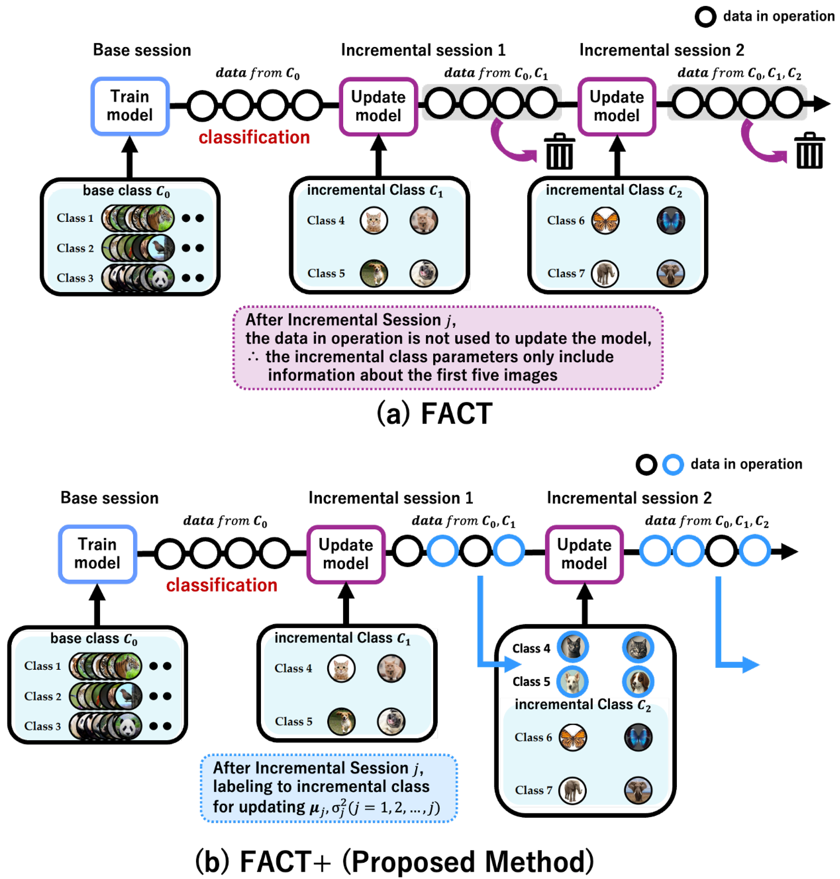Figure 1 illustrates a comparison between the proposed method (FACT+) and the original FACT framework. In terms of objective (2), FACT discards the data acquired during inference without using it for model updates as shown in Figure 1a. In contrast, FACT+ incorporates a mechanism to update only the incremental classes (indicated by the blue circles in Figure 1b), while keeping the base classes fixed (black circles in Figure 1b).

3.2. Incorporating Flexible Variance

We define the covariance matrix of a base class $c_i\in {\mathcal{C}}_0$ and that of an incremental class $c_j\in {\mathcal{C}}_1\cup \cdots \cup {\mathcal{C}}_b$ as ${\mathbf{\Sigma }}_i={\sigma }_i^2\mathbf{I}$ and ${\mathbf{\Sigma }}_j={\sigma }_j^2\mathbf{I}$, respectively (${\sigma }_i^2,{\sigma }_j^2\in {\mathbb{R}}^{+}$, $\mathbf{I}$: the identity matrix). The variance ${\sigma }_i^2$ of base class $c_i$ is treated as a learnable parameter from the base session, and the variance ${\sigma }_j^2$ of incremental class $c_j$ is computed in the b-th incremental session using:

$${\sigma }_j^2={\displaystyle \frac{1}{N_j^b}}\sum _{(\mathit{x},y^b)\in {\mathcal{D}}_b}\mathbb{I}(y^b=j)·\left|\right|\varphi \left(\mathit{x}\right)-{\mathit{w}}_j{\left|\right|}_2^2.$$

(13)

3.3. Model Update Using Post-Classification Data

While the model is in operation, we collect labeled data for incremental classes after classification and use it to update the model parameters.

More concretely, consider updating the model in the b-th incremental session. Let the set of incremental classes for which data annotation is performed be ${\mathcal{C}}_b^{\prime }={\bigcup }_{k=1}^{b-1}{\mathcal{C}}_k$. During the inference session immediately following the b-th incremental session, the input data consists of samples from both base classes and the newly added incremental classes. Each data point is labeled with one of the classes in ${\mathcal{C}}_b^{\prime }\cup \left\{[\mathrm{N}/\mathrm{A}]\right\}$. Here, “[N/A]” indicates that the data does not belong to any of the classes in ${\mathcal{C}}_b^{\prime }$. Consequently, data belonging to the base classes are labeled as “[N/A]” and are not utilized for model updates. If the assigned label is not “[N/A],” we use that data for model updates (In practice, we explore multiple scenarios for selecting which data points to use for model updates, but we introduce only one scenario here due to space constraints).

Suppose $\alpha$ data points are labeled with an incremental class $c_j\in {\mathcal{C}}_1\cup \cdots \cup {\mathcal{C}}_b$. Using Equations (5) and (13), we compute the new estimates of the prototype and variance, denoted ${{\mathit{w}}_j}^{\prime }$ and ${{\sigma }_j^2}^{\prime }$. We then update ${\mathit{w}}_j$ and ${\sigma }_j^2$ as follows:

$${\mathit{w}}_j\leftarrow {\displaystyle \frac{T_j^{b-1}}{T_j^{b-1}+\alpha }}{\mathit{w}}_j+{\displaystyle \frac{\alpha }{T_j^{b-1}+\alpha }}{{\mathit{w}}_j}^{\prime },$$

(14)

$${\sigma }_j^2\leftarrow {\displaystyle \frac{T_j^{b-1}}{T_j^{b-1}+\alpha }}{\sigma }_j^2+{\displaystyle \frac{\alpha }{T_j^{b-1}+\alpha }}{{\sigma }_j^2}^{\prime }.$$

(15)

Here, $T_j^{b-1}={\sum }_{k=1}^{b-1}{N}_j^k$ denotes the cumulative number of data points observed for class $c_j$ before the b-th session.

4. Experimental Evaluation

In this chapter, we conduct experiments to evaluate the effectiveness of the proposed method on a multi-class classification task under the CIL setting.

4.1. Experimental Setting

The dataset used in this experiment is CIFAR-100 [36], an image dataset consisting of color photographs of objects such as animals, plants, equipment, and vehicles.

Table 1. CIFAR-100 Class List [36].

Superclass	(Sub) Class
0: aquatic mammals	4: beaver, 30: dolphin, 55: otter, 72: seal, 95: whale
1: fish	1: aquarium fish, 32: flatfish, 67: ray, 73: shark, 91: trout
2: flowers	54: orchids, 62: poppies, 70: roses, 82: sunflowers, 92: tulips
3: food containers	9: bottles, 10: bowls, 16: cans, 28: cups, 61: plates
4: fruit and vegetables	0: apples, 51: mushrooms, 53: oranges, 57: pears, 83: sweet peppers
5: household electrical devices	22: clock, 39: computer keyboard, 40: lamp, 86: telephone, 87: television
6: household furniture	5: bed, 20: chair, 25: couch, 84: table, 94: wardrobe
7: insects	6: bee, 7: beetle, 14: butterfly, 18: caterpillar, 24: cockroach
8: large carnivores	3: bear, 42: leopard, 43: lion, 88: tiger, 97: wolf
9: large man-made outdoor things	12: bridge, 17: castle, 37: house, 68: road, 76: skyscraper
10: large natural outdoor scenes	23: cloud, 33: forest, 49: mountain, 60: plain, 71: sea
11: large omnivores and herbivores	15: camel, 19: cattle, 21: chimpanzee, 31: elephant, 38: kangaroo
12: medium-sized mammals	34: fox, 63: porcupine, 64: possum, 66: raccoon, 75: skunk
13: non-insect invertebrates	26: crab, 45: lobster, 77: snail, 79: spider, 99: worm
14: people	2: baby, 11: boy, 35: girl, 46: man, 98: woman
15: reptiles	27: crocodile, 29: dinosaur, 44: lizard, 78: snake, 93: turtle
16: small mammals	36: hamster, 50: mouse, 65: rabbit, 74: shrew, 80: squirrel
17: trees	47: maple, 52: oak, 56: palm, 59: pine, 96: willow
18: vehicles 1	8: bicycle, 13: bus, 48: motorcycle, 58: pickup truck, 90: train
19: vehicles 2	41: lawn-mower, 69: rocket, 81: streetcar, 85: tank, 89: tractor

shows a list of the classes in CIFAR-100. Following previous work [15], we split the dataset so that classes with IDs 0–59 are treated as base classes, and those with IDs 60–99 are incremental classes. Each base class contains 500 data points, and each new incremental class introduced for the first time in any incremental session contains five data points. We add five classes per incremental session, for a total of eight incremental sessions, and evaluate accuracy across all nine sessions (including the base session).

We train for 600 epochs with a batch size of 256 and set the learning rate in the base session to 0.01. We use stochastic gradient descent for optimization [37] and adopt ResNet20 [38] as the encoder. All experiments were conducted on a workstation equipped with an Intel (Santa Clara, CA, USA) Core i9-9900K CPU (3.6 GHz, 8 cores), an NVIDIA (Santa Clara, CA, USA) GeForce GTX 1660 SUPER GPU (6 GB VRAM), and 64 GB of system memory.

To investigate the significance of each proposed component through an ablation study, we compare four models whose configurations are summarized in

Table 2. List of the model configurations.

Model	Flexible Covariance Matrices	Dynamically Model Update
1. FACT
2. FACT+ w/o update	✓
3. FACT+ w/o dynamic-var		✓
4. FACT+	✓	✓

.

4.2. Experimental Results

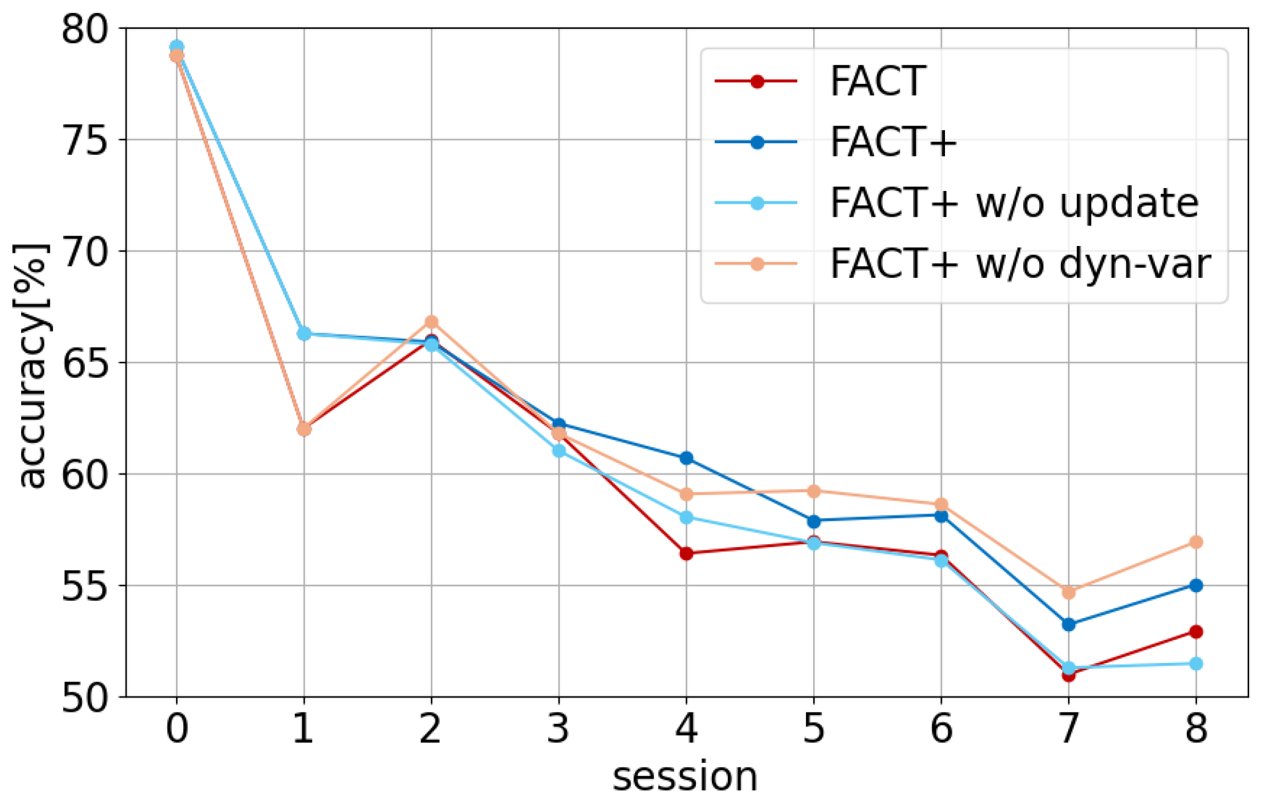
Figure 2 shows the classification accuracy of each model. The base session is labeled as session 0, and incremental sessions are labeled as 1–8.

From Figure 2, we see that FACT+ w/o update surpasses FACT in some sessions (sessions 0, 1, 4, 7). Moreover, the proposed method (FACT+) outperforms FACT in 8 out of 9 sessions. This suggests that introducing flexible variance improves accuracy for some classes, and using deployment data to update the parameters effectively supplements knowledge about incremental classes with limited initial data, helping maintain higher accuracy in later sessions.

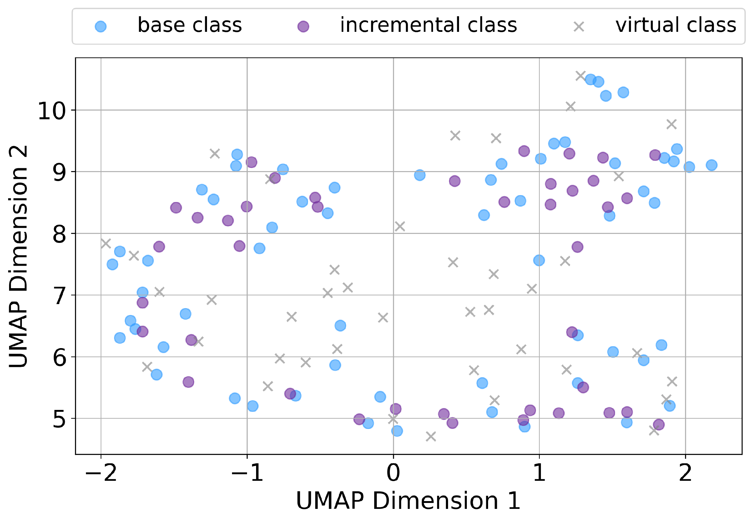
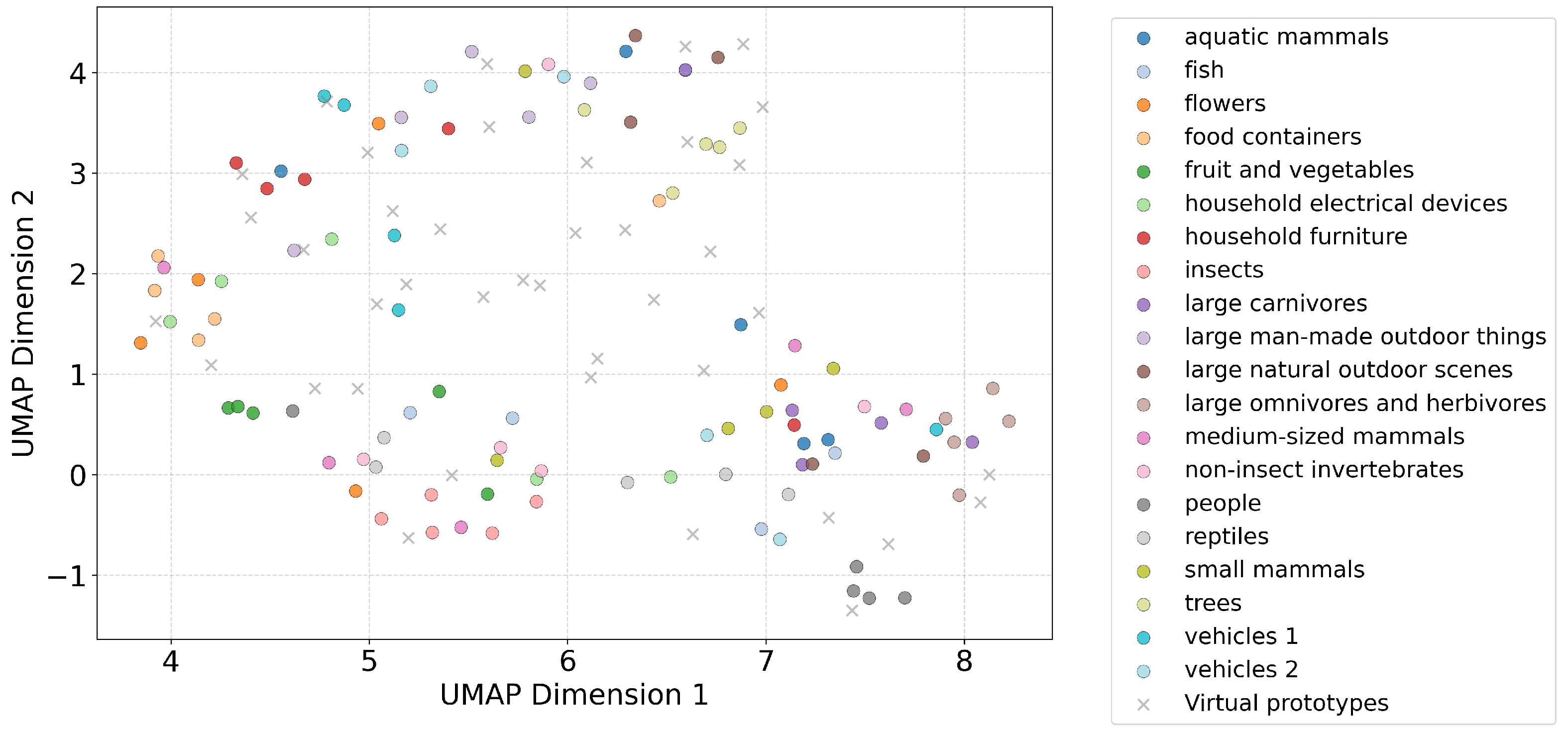
Next, we visualize the embedding space learned by FACT+ to examine how class prototypes are organized after training and incremental updates. Figure 3 shows the prototypes categorized by their class type (base, incremental, and virtual), whereas Figure 4 groups them by the 20 superclasses defined in CIFAR-100. Both figures present two-dimensional UMAP [39] projections of the learned prototypes.

In Figure 3, blue, purple, and gray points denote the prototypes of base, incremental, and virtual classes, respectively. Observing Figure 3, it can be seen that semantically related base and incremental classes are embedded in close proximity within the embedding space. While the base classes are sufficiently learned by the model, the incremental classes are not explicitly trained but are instead obtained solely through the use of the pretrained encoder. Even with the introduction of class-specific variances in the proposed method, no distortion or bias was observed in the spatial arrangement of either the base or incremental classes. These observations indicate that the validity of the embedding space obtained through FACT+ is well preserved.

Figure 4 colors each class prototype according to the 20 superclasses defined in CIFAR-100. The color legend corresponds to the 20 superclasses defined in Table 1. The order of the legend items is consistent with the superclass IDs in the table (e.g., 0: aquatic mammals, 1: fish, …, 19: vehicles 2). Prototypes belonging to the same superclass tend to be embedded in close proximity within the embedding space. For instance, food containers (center-left), household furniture (upper-left), people (lower-right), and trees (upper-center) each form a compact cluster. The virtual prototypes (gray “×”) are interspersed across regions, bridging semantically related classes without forming a dominant cluster.

These results confirm that FACT+ effectively captures semantic consistency across both previously learned and newly introduced classes, producing an embedding space that preserves meaningful organization.

5. Discussion

In this chapter, we conduct additional experiments and analyses under various conditions to more comprehensively evaluate our proposed method, FACT+.

In Section 5.1, we compare the computational complexity, memory cost, and runtime between FACT and FACT+. Then, in Section 5.2 and Section 5.3, we compare the classification accuracy of each model on characteristic datasets (data with different class hierarchies and data where the features of base and incremental classes differ significantly). In Section 5.4, we compare the accuracy of our proposed model with a model where the covariance matrices for virtual classes are also variable, in addition to those for base and incremental classes. This allows us to verify the validity of only varying the covariance matrices for base and incremental classes. Finally, in Section 5.5, we discuss the model’s sensitivity to the quality and amount of both training and post-deployment data.

5.1. Computational Complexity, Memory Cost, and Runtime Analysis

The number of model parameters for FACT and FACT+ is compared in

Table 3. Breakdown of parameters used in FACT and FACT+.

Component	FACT	FACT+
Encoder	ResNet20 $271,824$	ResNet20 $271,824$
Base session	prototypes $64\times 60$	prototypes $64\times 60$ + variances 60
Incremental sessions	prototypes $64\times 40$	prototypes $64\times 40$ + variances 40
Total parameters	$278,224$	$278,324$

. Introducing class-specific covariance (variance) parameters in FACT+ leads to only a marginal increase in parameter count (Increase: only 0.00036%). Accordingly, the memory cost and computational load remain almost unchanged in theory. However, FACT+ involves the Mahalanobis distance calculation, which requires additional matrix inversion steps during both training and inference.

To quantify this additional cost, we also measured the actual computation times. For the base session (training on Session 0), FACT required approximately 24,169 s (≈6.7 h), while FACT+ took 24,436 s (≈6.8 h)—an increase of only about 1%. For inference across the incremental sessions (Sessions 1–8), the total computation time was 611 s (≈10 min) for FACT and 800 s (≈13 min) for FACT+, reflecting a modest rise mainly due to the Mahalanobis distance computation during prediction. Overall, the additional complexity in FACT+ introduces only a minor runtime overhead while maintaining nearly identical memory consumption to FACT.

While this additional computation time is relatively small, it may become non-negligible for large-scale datasets. Exploring optimization strategies to reduce this overhead remains a promising direction for future research.

5.2. Validation with Data of Varying Class Granularity

5.2.1. Experimental Setting

The CIFAR100 dataset is organized into 20 superclasses, each consisting of five subclasses (totaling 100 classes). We first select 10 superclasses as ${\mathcal{C}}^{\mathrm{high}}$ and take the subclasses under the remaining 10 superclasses—that is, 50 subclasses—as ${\mathcal{C}}^{\mathrm{low}}$. Our training dataset is then constructed to include both large-grained (higher-level) classes and small-grained (lower-level) classes. Specifically, the base session includes six classes from ${\mathcal{C}}^{\mathrm{high}}$ and 30 classes from ${\mathcal{C}}^{\mathrm{low}}$. Each incremental session adds one new class from ${\mathcal{C}}^{\mathrm{high}}$ and five new classes from ${\mathcal{C}}^{\mathrm{low}}$.

We simulate a scenario of one base session followed by four incremental sessions, each adding six classes. Regardless of class granularity, each base class has 500 data points, and each incremental class has five data points, randomly chosen. Other settings (optimizer, encoder, etc.) follow Section 4.1, and we use FACT+ as the model.

5.2.2. Experimental Results

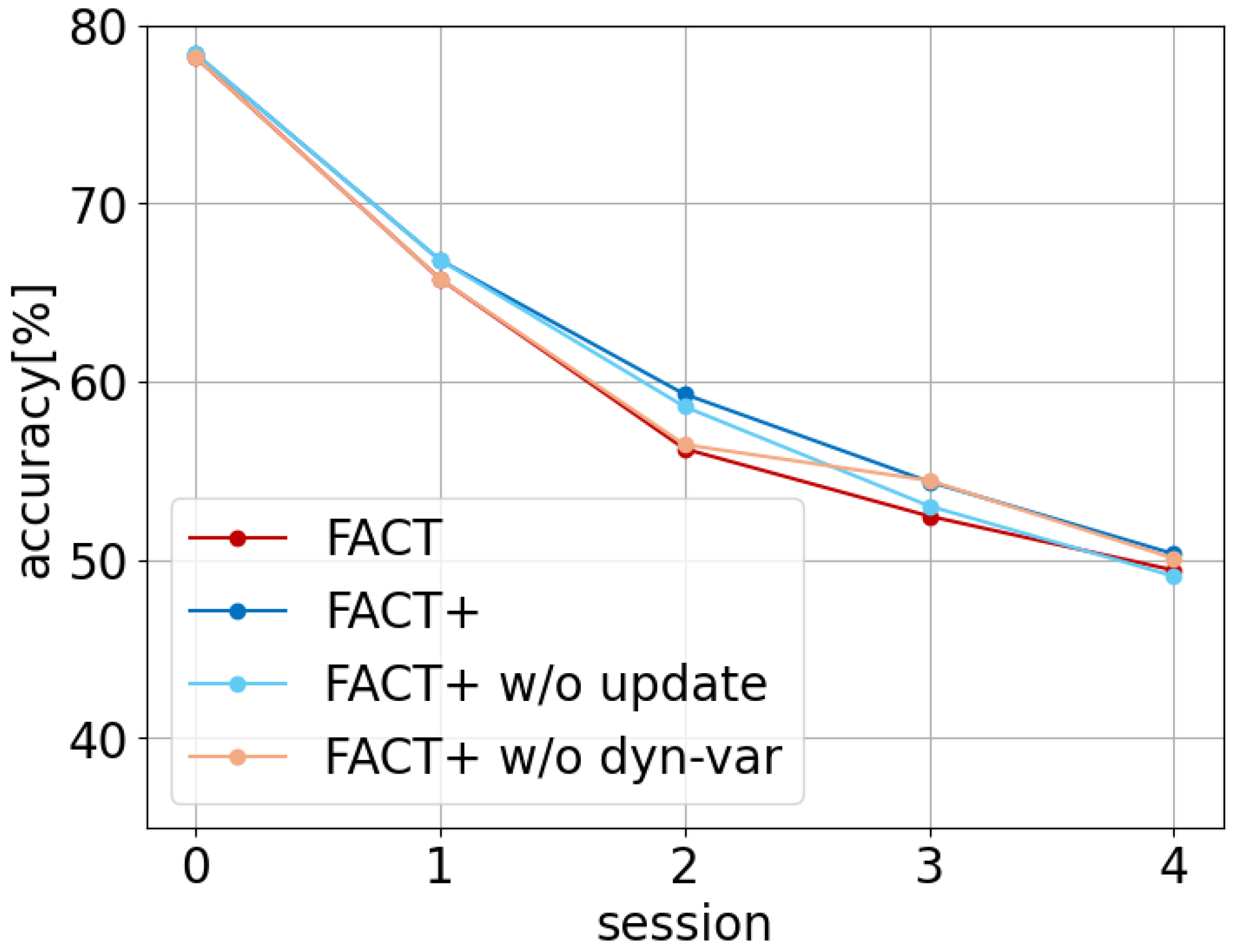
Figure 5 shows the accuracy comparisons of each model. Session 0 is the base session, and sessions 1–4 are incremental.

From Figure 5, FACT+ outperforms FACT in all sessions. Comparing FACT+ and FACT+ w/o dynamic-var, both of which reuse data, FACT+ exhibits higher accuracy in four of the five sessions. This indicates that flexible variance is effective when classes differ significantly in their semantic diversity.

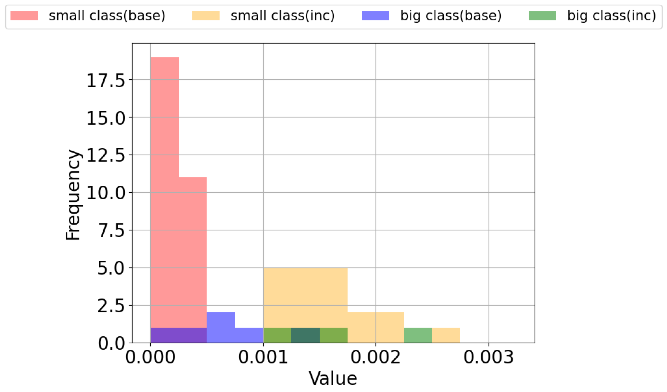
Next, Figure 6 shows the distribution of variance values for each class $c_i\in {\mathcal{C}}_0\cup \cdots \cup {\mathcal{C}}_4$. From Figure 6, the variances for base classes are generally smaller for lower-level classes and larger for higher-level classes. At the end of session 8 in FACT+, the average variance for the higher-level base classes is $6.91\times {10}^{-4}$, whereas it is $2.00\times {10}^{-4}$ for the lower-level base classes. For incremental classes, the average variance for higher-level classes is $1.64\times {10}^{-3}$ and $1.48\times {10}^{-3}$ for lower-level classes. Notably, for the base classes in particular, the method successfully infers a larger variance for classes with broader semantic diversity and a smaller variance for classes with narrower diversity.

Combining these findings with the results in Section 4.2 (“flexible variance boosts accuracy for certain classes”), it can be inferred that effective estimation of variance has a positive impact on predictive performance.

However, as shown in Figure 6, not all superclasses had larger variances than all subclasses. One possible reason is the limited number of data points for incremental classes. In this experiment, following Zhou et al. [15], the number of data points for superclasses was matched to that of subclasses, meaning that the number of data points for incremental class $c_j\in {\mathcal{C}}_b$ newly added to the model in session b is $N_j^b=5$. This implies that among the five subclasses grouped as a superclass, there might be classes not included in the incremental session’s data, suggesting insufficient data points for calculating incremental class parameters.

In the experiments in Section 5.2.2, our aim was to evaluate the model’s robustness under scenarios where various types of classes could be introduced. The thing to note here is that the proposed model does not currently embed hierarchical class relationships. In real-world scenarios, however, incremental classes may appear in strict inclusion or hierarchical relationships with previously learned base classes. Therefore, integrating the proposed approach with models that explicitly encode hierarchical or nested structures—such as box-based hierarchical embeddings [40,41]—remains an open and promising direction for future investigation.

5.3. Validation with Datasets Where Base and Incremental Class Features Differ Significantly

This section verifies that the proposed method’s mechanism functions effectively in situations where the features of base classes and incremental classes differ significantly. In the experimental conditions of Section 5.4.1, CIFAR100 class numbers were assigned randomly regardless of class category, so there was no bias towards similar classes being grouped into either base or incremental classes. However, in practical applications, the types of base and incremental classes may be entirely different, potentially leading to inaccurate embedding representations for incremental classes if the encoder trained on base classes cannot adequately handle them. For example, a user who has previously photographed and stored many images of people might suddenly become interested in trains or airplanes. As photos of these new subjects accumulate in their folders, they need to be appropriately tagged. To simulate such a scenario, this experiment artificially assigns base and incremental classes within CIFAR100 to reproduce a dataset where the features of base and incremental classes differ significantly.

5.3.1. Experimental Setting

Based on the superclasses of CIFAR100 (20 categories in the dataset) as shown in Table 1, the dataset was split such that base classes comprised natural objects like animals and plants (superclasses: 0, 1, 2, 3, 4, 7, 8, 9, 10, 11, 12, 13), and incremental classes comprised people or artificial objects (superclasses: 5, 6, 14, 15, 16, 17, 18, 19). This setup establishes a configuration where the types of base and incremental classes differ significantly. Other experimental conditions are the same as those described in Section 4.1.

5.3.2. Experimental Results

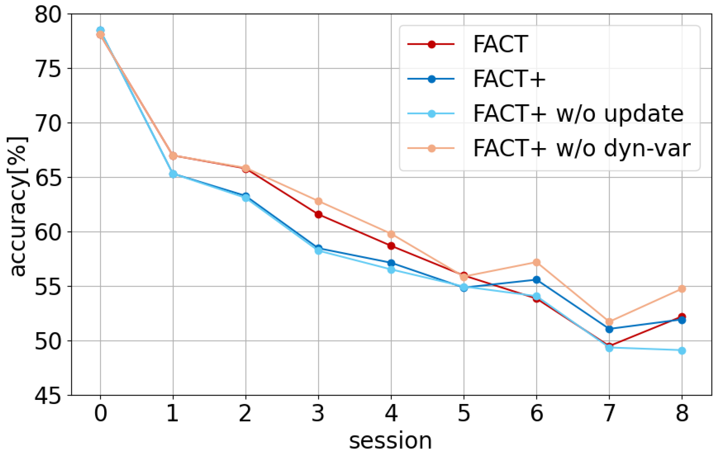
Figure 7 shows the comparison of accuracy for each model. From Figure 7, it can be observed that FACT+ w/o dynamic-var outperforms FACT in classification accuracy in eight out of nine sessions. This suggests that incorporating a data reuse mechanism can suppress the decrease in accuracy to some extent, even when incremental classes with low similarity to base classes appear. On the other hand, FACT+ only surpassed FACT’s accuracy in sessions 6 and 7. From this result, it is suggested that while the data reuse mechanism functions well in cases where base and incremental class features differ significantly, as in this experiment, introducing dynamic variance is not effective.

5.4. Application of Dynamic Variance to Virtual Classes

In the proposed method, the covariance matrices of base and incremental classes were variable, but the covariance matrix of virtual classes was fixed as an identity matrix. This section investigates how varying the covariance matrix of virtual classes, ${\mathbf{\Sigma }}_v$, affects accuracy and discusses the contributing factors.

5.4.1. Experimental Setting

In this experiment, a model with a variable covariance matrix for virtual classes (FACT+ w/o update w/ variable-${\sigma }_v$) is introduced as a new comparison method. In this model, in addition to ${\mathbf{\Sigma }}_i$ and ${\mathbf{\Sigma }}_j$ (${\sigma }_i^2,{\sigma }_j^2\in \mathbb{R}$, $\mathbf{I}$: identity matrix on ${\mathbb{R}}^{d\times d}$), the covariance matrix of a virtual class ${\mathit{p}}_v\in {\mathcal{C}}_v$ is defined as ${\mathbf{\Sigma }}_v={\sigma }_v^{2}I({\sigma }_v^2\in \mathbb{R})$. The variances of base classes ${\sigma }_i^2$ and virtual classes ${\sigma }_v^2$ are learning parameters in the base session, and the variances of incremental classes are calculated in the incremental session. In this experiment, FACT+ w/o update is used as a comparison model, and the data reuse mechanism is not introduced; only the variability of variance is manipulated. Other experimental conditions are the same as those described in Section 4.1.

5.4.2. Experimental Results

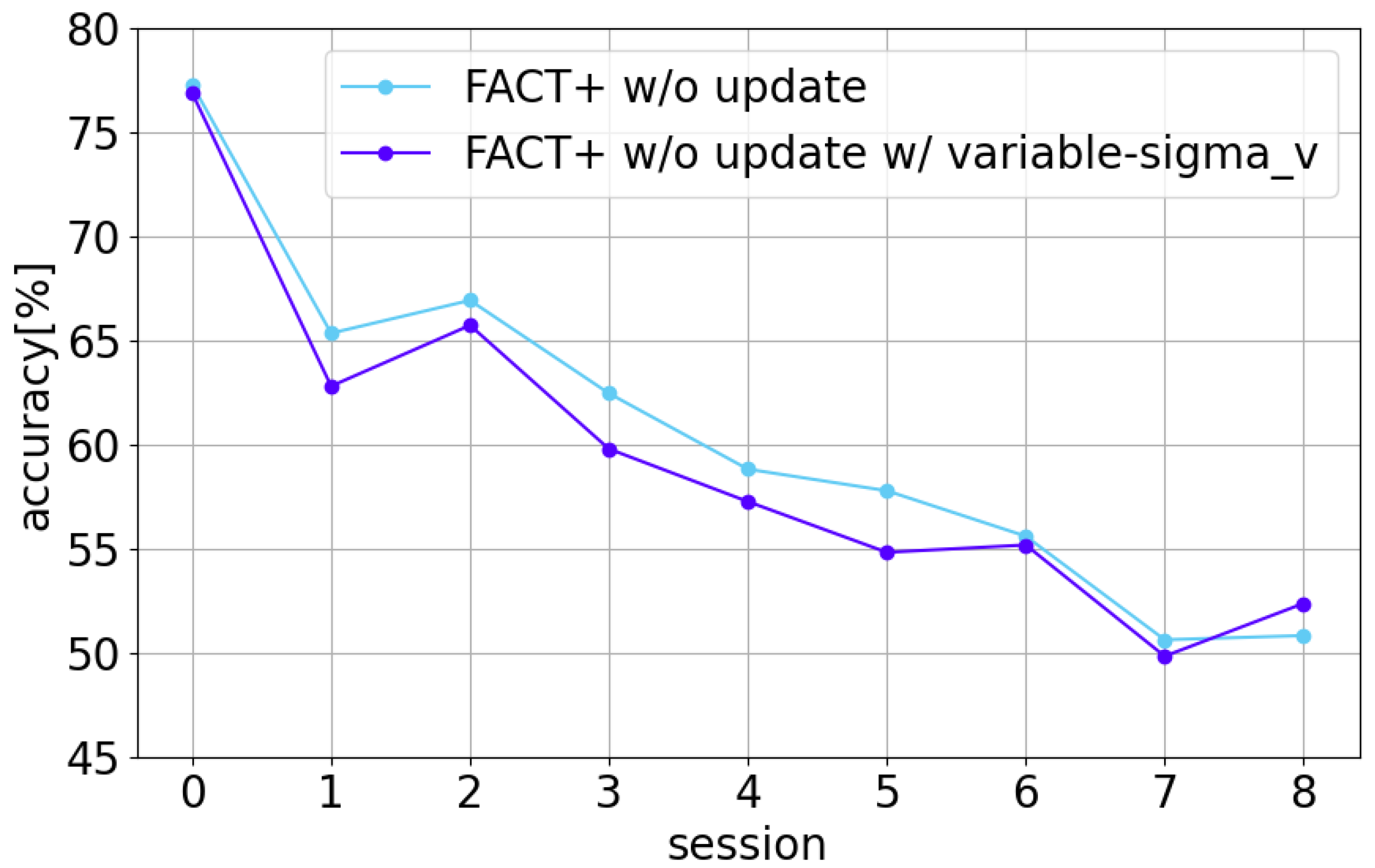
Figure 8 shows the comparison of accuracy for each model. From Figure 8, FACT+ w/o update w/ variable-${\sigma }_v$ underperformed FACT+ w/o update in eight out of nine sessions.

The following two points are inferred as the reasons why the accuracy trend of FACT+ w/o update w/ variable-${\sigma }_v$ was unstable and no improvement in accuracy was observed. The first point is the increase in the number of learning parameters. Generally, as the number of learning parameters in a machine learning model increases, its expressive power improves, but the possibility of overfitting to the training data also increases [42]. Moreover, learning can become unstable as the number of learning parameters increases [38,43]. The second point is the structure of the likelihood calculation in the proposed method. The probability density function of the normal distribution, given by Equations (9) and (10), includes the matrix norm of the covariance matrix in the denominator. Specifically, it contains the structure shown in the following Equation (16).

$$p\left({\mathit{w}}_i\right|{\mathit{p}}_v)={\displaystyle \frac{1}{\sqrt{{\left(2\pi \right)}^n\left|{\mathbf{\Sigma }}_v\right|}}}exp\left(-{\displaystyle \frac{1}{2}}{({\mathit{w}}_i-{\mathit{p}}_v)}^{\top }{\mathbf{\Sigma }}_v^{-1}({\mathit{w}}_i-{\mathit{p}}_v)\right).$$

(16)

In Equation (16), it is known that if ${\mathbf{\Sigma }}_v\in {\mathbb{R}}^{d\times d}$ becomes a high-dimensional variable, the likelihood calculation becomes unstable due to the curse of dimensionality [44,45,46].

Therefore, it is inferred that the magnitude of the variance significantly affects likelihood calculation, leading to instability, increased misclassifications, and thus a decline in classification performance. Fundamentally, unlike base and incremental classes, virtual classes are not tied to specific concrete classes, so considering the magnitude of their variance is thought to offer few advantages. Based on this result, the proposed method fixes the variance of virtual classes to an identity matrix.

5.5. Noise Sensitivity and Data Quality

Regarding image noise, CIFAR-100 [36] consists of real-world photographs annotated with class labels; thus, some level of variation inherent in everyday image capture (e.g., lighting, background, or angle) is already reflected in the dataset. For label noise, CIFAR-100 is also known to contain mislabeled samples [47]. The proposed model maintained stable performance under these conditions, suggesting a certain degree of robustness to moderate noise in both inputs and labels.

Furthermore, the effectiveness of continual updates may depend on both the amount and quality of post-deployment data. Although this study mainly focused on verifying the model’s update mechanism, it is reasonable to assume that the quantity of update data would influence performance. Similarly, data quality—specifically, the informativeness and representativeness of samples—could have a comparable effect. This aspect is discussed further in relation to active learning strategies in Section 6.

6. Conclusions and Future Work

In this work, we proposed FACT+, a novel model that extends the Forward Compatible Few-Shot Class-Incremental Learning (FACT) framework with two key improvements.

First, we addressed the limitation of FACT’s assumption that all classes have a uniform Gaussian distribution in the embedding space, which hinders the model’s ability to capture the semantic diversity of each class. To overcome this, FACT+ introduces learnable variance–covariance matrices for each class’s embedding region. This flexibility allows the model to better reflect the true semantic scope of each class, from broad categories to narrow sub-classes.

Second, we tackled the challenge of improving classification performance for incremental classes after the initial few-shot learning. The original FACT model, once deployed, cannot refine its knowledge of new classes as more data becomes available. In contrast, FACT+ incorporates a mechanism for dynamically updating class prototypes and their variances using labeled data obtained during deployment. This capability allows the model to continuously adapt to and refine its understanding of new classes.

To validate the effectiveness of these improvements, we conducted a series of comprehensive experiments. We first confirmed that FACT+ achieves higher overall accuracy across most sessions compared to the original FACT model. This success is attributed to our model’s ability to secure embedding regions that accurately reflect the semantic diversity of each class and its capability to continuously supplement knowledge about incremental classes during deployment.

Future directions include model compression and exploring more effective annotation strategies. Since introducing flexible variance in the proposed model increases the number of parameters in proportion to the number of classes and necessitates additional variance calculations, reducing memory usage and computational overhead is desirable. Lightweight compression approaches such as parameter pruning, low-rank factorization, or knowledge distillation could be explored to reduce memory and computational requirements without significant loss of accuracy. Although their feasibility within the proposed framework has not yet been verified, this represents a promising direction worth investigating to improve scalability.

Additionally, incorporating active learning techniques has the potential to further enhance the effectiveness of model updates. In this study, we introduced a mechanism that reuses post-deployment data for continual model updates. However, in the current implementation, all newly collected data are treated equally, without considering their informativeness or reliability.

As discussed above, the effectiveness of updates may also depend on the quality of the data used—particularly, whether the samples provide valuable information for refining class boundaries or reinforcing representative prototypes. Active learning offers a promising way to address this issue by selectively leveraging such high-value samples. For instance, prioritizing uncertain or boundary samples may strengthen class separation, whereas selecting representative samples near class prototypes could improve stability during updates. While the practical impact of these strategies remains to be validated, they represent a natural extension of the current framework toward more efficient and robust continual adaptation.

Finally, although our experiments considered classes of different granularity that do not form a strict hierarchical or inclusion relationship, testing the proposed method under scenarios where classes are in an inclusion relationship remains an important area for future investigation.