Article

An Interval-Valued Neutrosophic Framework: Improved VIKOR with a Preference-Aware AHP–Entropy Weight Method for Evaluating Scalp-Detection Algorithms

International Cooperation Center for Design Strategy of Guangdong, Hong Kong and Macao Greater Bay Area, School of Design, South China University of Technology, Guangzhou 510641, China
*
Author to whom correspondence should be addressed.
Appl. Sci. 2025, 15(22), 11937; https://doi.org/10.3390/app152211937
Submission received: 6 October 2025 / Revised: 4 November 2025 / Accepted: 5 November 2025 / Published: 10 November 2025
(This article belongs to the Special Issue Applications of Fuzzy Systems and Fuzzy Decision Making)

Abstract

Scalp image detection faces challenges such as limited evaluation dimensions, difficulties in quantifying user perception, and insufficient discriminative power of traditional assessment methods. To address these issues, this paper proposes a multi-attribute decision-making model for deep learning algorithm selection. The model integrates subjective and objective weighting through a hybrid approach, where natural language processing (NLP) techniques extract perceptual preferences from user reviews, and the Interval-valued neutrosophic set analytic hierarchy process (IVNS-AHP) and entropy weight method (EWM) are employed to determine subjective and objective weights, respectively. The combined weights are used within the IVNS-VIKOR (Vlse Kriterijumska Optimizacija Kompromisno Resenje) framework, enhanced by a possibility distribution (PD) to improve discriminative capability. Experiments were conducted using multiple performance metrics, including Precision, Recall, mean Average Precision at IoU = 0.5 (mAP@50), F1 Score, frames per second (FPS), and Parameters, to evaluate mainstream scalp detection algorithms. The results demonstrate that YOLOv8n achieves the highest comprehensive ranking with strong stability across different decision preferences. Comparative analyses with TODIM (an acronym in Portuguese of interactive and multiple attribute decision-making), TOPSIS (Technique for Order Preference by Similarity to an Ideal Solution), and fuzzy VIKOR variants confirm that the proposed PD-VIKOR method provides superior ranking stability and discriminative precision, offering a more reliable and robust evaluation under uncertainty.

1. Introduction

1.1. Background

Driven by national strategies such as the “Healthy China 2030” Outline and the “14th Five-Year Plan for National Health Informatization,” the concept of “comprehensive health” is profoundly reshaping public health management models in China, propelling a shift from passive treatment to proactive monitoring and self-management [1,2]. This trend has accelerated the development of smart health monitoring devices that integrate physiological sensing with artificial intelligence. Among these, the scalp health monitor stands out as a tool for personalized health care. Its core technology lies in analyzing scalp images to achieve precise quantification of physiological states and identification of pathological features.
As public health literacy improves, users’ demands for devices have moved beyond basic functionality, shifting instead to a greater focus on core performance metrics such as detection accuracy, response speed, ease of operation, and personalized service capabilities [3]. In the field of light medical aesthetics, such as scalp analyzers, “user experience first” has replaced single precision metrics as the new standard for evaluating device efficacy [4]. This shift demands multidimensional optimization in product design and drives algorithm selection away from pursuing “single-performance optimization” toward systematic decision-making based on “multidimensional user satisfaction” [5].
Product algorithm selection is fundamentally a multi-attribute group decision-making (MAGDM) problem, whose core lies in coordinating group decision-makers and comprehensively balancing multidimensional technical metrics with user subjective perceptions [6,7]. However, traditional decision-making models struggle to effectively address the widespread subjective ambiguity, scoring uncertainty, and group cognitive conflicts inherent in such decisions [8,9,10]. Therefore, how to construct a comprehensive evaluation framework that scientifically balances technical performance and user experience has become a critical issue requiring urgent resolution in this field.

1.2. Literature Review

In recent years, with the rapid increase of user-generated content and the advancement of artificial intelligence technologies, Natural language processing (NLP) methods, particularly text mining and sentiment analysis, have been increasingly applied in multi-attribute decision support systems. Compared with traditional survey-based approaches that rely on structured questionnaires or interviews, these techniques are widely recognized for their ability to extract authentic and real-time user preferences directly from large volumes of unstructured data [11]. For example, Zheng et al. [12] developed a sentiment interpretation model based on the Circular Pythagorean Fuzzy Set to optimize deep learning structure decisions, demonstrating the feasibility of transforming user reviews into effective decision inputs. Similarly, Yadav et al. [13] embedded sentiment scores extracted from online reviews into AHP-VIKOR and IF-MOORA models to comprehensively rank mobile payment platforms, thereby validating the adaptability of user semantic information in multi-criteria evaluation. However, despite these attempts to incorporate user sentiment into decision-making, existing studies still lack quantitative mechanisms derived from actual semantic feedback, which limits the realization of a truly user-centered model orientation [14]. Furthermore, many approaches continue to rely on traditional fuzzy set or intuitionistic fuzzy set theories, which may lead to semantic distortion and dimensional compression when representing user hesitation and emotional fluctuation [15], thus constraining the model’s capability to accommodate heterogeneous and multi-source information.
Previous studies have attempted to enhance the adaptability of decision-making models under uncertainty by extending fuzzy set theories, particularly in the integration of multi-source heterogeneous information and the representation of expert hesitation in scoring. Zhang et al. [16] addressed the product ranking problem of large-scale online reviews on e-commerce platforms by incorporating prospect theory into the VIKOR framework and developing a novel sentiment analysis algorithm. This approach strengthened the influence of user emotions on satisfaction computation while introducing a hybrid weighting mechanism that combines collective entropy weights with individual subjective preferences. Although this method effectively improved the personalization and dynamism of consumer satisfaction modeling, it still required explicit control over membership adjustment and exhibited limited capability in representing rating fuzziness and hesitation. Alamoodi et al. [17] constructed a two-stage weighting–ranking model (NS-FWZIC and NS-FDOSM) within a neutrosophic set environment for intelligent tourism recommendation systems. By managing the fluctuation of expert cognition, their approach achieved evaluation stability across heterogeneous application domains. However, the neutrosophic set adopted in their model was a simplified form, which failed to fully capture the coexistence of “support–opposition–hesitation” semantics in non-complementary cognitive structures, thereby constraining its generalization ability in complex opinion fusion scenarios.
As a generalized extension of fuzzy set theory, the IVNS models truth-membership, falsity-membership, and indeterminacy-membership as three independent functions, effectively overcoming the limitation of single-dimensional representation in traditional fuzzy sets. Unlike fuzzy sets and intuitionistic fuzzy sets, IVNS allows these three cognitive components to vary independently within the interval [0, 1] without satisfying any complementary constraint. This feature enables IVNS to represent evaluative attitudes under complex cognitive conditions more realistically, such as situations where “partial agreement,” “partial disagreement,” and “indecisiveness” coexist [18]. With these advantages, IVNS provides greater flexibility and interpretability when dealing with conflicting expert opinions, vague user evaluations, and incomplete information. In practical applications, IVNS has been extended into several variants, including weighted, probabilistic, and hesitant formulations. Zhang et al. [19] addressed the MAGDM requirements for agricultural B2C e-commerce service quality by proposing a “CRITIC weighting and IVIFS-GRA” framework, which effectively ranked and optimized service alternatives. Numerical and comparative experiments confirmed its validity and provided a feasible assessment approach for this field. Liu et al. [20] developed a hybrid MAGDM model under the IVIFS environment by integrating the IVIFWA aggregation operator, correlation-based expert weighting, and variable attribute weighting within a TOPSIS framework. Two numerical examples demonstrated its higher effectiveness and more stable ranking performance compared with traditional methods. Similarly, Zhou et al. [21] proposed a regional sustainability assessment model for the water–land–energy–carbon (WLEC) coupling system based on IVIFS and MAGDM. The application to Heilongjiang Province revealed notable intercity differences in coupling levels and yielded policy recommendations suggesting that groundwater utilization rates should be maintained within the range of 16% to 28%.
To further enhance the applicability of IVNS in the ranking stage of MAGDM, researchers have integrated it with improved VIKOR methods, particularly by incorporating possibility theory to strengthen the ranking capability under highly uncertain or hesitant information. Wang et al. [22] proposed a VIKOR method under a circular intuitionistic fuzzy (C-IF) environment by introducing an enhanced score function and a modified Chebyshev distance, which jointly characterize membership, non-membership, and information reliability while integrating radial features. The method achieved more robust superiority identification and compromise ranking in a medical waste disposal case. Hendiani et al. [23] developed a VIKOR model based on the interval-valued q-rung orthopair fuzzy set (IVq-ROFS) using a dual-layer possibility and neutralized decision matrix. This approach eliminated the need for conventional normalization and calculated utility and compromise measures through cumulative possibility–weight interactions, yielding a unique and distinguishable ranking with higher robustness in group decision contexts. Chen et al. [24] addressed the issues of zero-radius failure and semantic loss in the relative scoring of C-IF VIKOR by proposing a new score function with scale and exponential parameters, coupled with a C-IF Minkowski distance to form a parameterized VIKOR model. This model flexibly balanced utility, regret, and compromise effects, and demonstrated strong adaptability and stability in applications such as site selection, supplier evaluation, and medical waste technology assessment.

1.3. Research Gap

The significance of intelligent health monitoring devices and image analysis algorithms has become increasingly prominent. However, most existing studies primarily focus on single-dimensional comparisons of algorithmic performance, such as improving recognition accuracy or optimizing computational complexity [25], while lacking a systematic and integrative evaluation framework that simultaneously incorporates algorithmic technical attributes and end-user perceptual dimensions.
Specifically, the limitations of current research can be summarized in three aspects.
(1)
From a methodological perspective, there is an absence of mature theoretical models capable of effectively addressing the inherent subjectivity, uncertainty, and group divergence in algorithm selection processes.
(2)
From a research perspective, algorithms are often treated merely as technical entities, neglecting their role as components of user-oriented products. This results in a disconnection between technical performance indicators and user satisfaction.
(3)
From an interdisciplinary application perspective, the systematic application of advanced fuzzy theoretical frameworks such as the IVNS to image detection algorithm evaluation remains largely unexplored [26]. This gap between theoretical development and practical implementation highlights the necessity and innovative value of the present study.

1.4. Research Contributions

In response to the existing limitations in methodology, research perspective, and interdisciplinary application, the contributions of this paper are reflected in three main aspects.
(1)
From a methodological standpoint, this paper integrates the AHP with the VIKOR method and extends it to the IVNS environment. Two types of possibility functions are further defined to enhance the VIKOR mechanism, significantly improving the precision of alternative comparison and the discriminative power of ranking. This provides a more robust theoretical tool for addressing the complex cognitive uncertainty inherent in algorithm selection.
(2)
From the perspective of research orientation, this paper introduces NLP techniques to construct a user-preference-oriented hybrid weighting approach that combines subjective and objective information. By structurally integrating multidimensional user experience indicators, the proposed framework shifts the decision-making focus from “technically optimal” to “user-satisfactory,” effectively bridging the gap between technical performance metrics and actual user perception.
(3)
From an interdisciplinary application perspective, this paper applies IVNS theory to the evaluation and selection of image detection algorithms for the first time. This work not only extends the application boundary of fuzzy decision-making theory but also provides a novel theoretical reference for the development of intelligent health terminal products that integrate both technical performance and user preference.

1.5. Organization

The remainder of this paper is structured as follows: Section 2 reviews text mining techniques and sentiment analysis methods in natural language processing, along with IVNS-related operations. Section 3 details the steps of the proposed method. Section 4 presents empirical research on this approach. Section 5 conducts sensitivity analysis and compares the proposed method with other approaches. Section 6 discusses the results.

2. Preliminaries

2.1. User Requirement Identification and Weighting Construction

2.1.1. TF-IDF (Term Frequency-Inverse Document Frequency) Weighting Technique

User review data was collected via web crawlers. Preprocessing steps included word segmentation, stopword removal, word frequency counting, and TF-IDF calculation (see [27,28]).
Term frequency (TF):
T F ( t , d ) = n N
where t represents a specific word, d represents the number of documents, n is the frequency of that term within the documents, and N is the total number of words in the documents.
TF-IDF:
T F - I D F ( t , d ) = T F ( t , d ) × log D 1 + d f ( t )
where D is the total number of documents in the corpus, and d f t is the number of documents containing term t.

2.1.2. LDA Topic Identification and Visualization

The Latent Dirichlet Allocation (LDA) model was employed for topic modeling [29], with its structural framework illustrated in Figure 1. The optimal number of topics was determined using perplexity and topic consistency:
Perplexity (see [30]):
P e r p l e x i t y ( D ) = exp ( d D log P ( w d ) d D N d )
where P ( w d ) is the joint probability of all words in document d, N d denotes the number of words in document d, d D N d is the total number of words across all documents.
Thematic Consistency (see [31]):
C ( W ) = j = 2 M i = 1 j 1 log D ( w i , w j ) + 1 / ε D ( w i )
where D ( w i ) denotes the number of documents containing, D ( w i , w j ) is the number of documents containing both w i   and w j , and 1 / ε   is the smoothing factor.

2.1.3. User Preference Weighting

To enhance the accuracy and domain adaptability of sentiment recognition, this paper utilizes Baidu’s NLP sentiment analysis API to process user review texts. The specific processing steps are outlined in Algorithm 1.
Algorithm 1: Sentiment Analysis Using Baidu NLP API
Input: Text content, API Key, Secret Key
Output: Sentiment polarity and confidence score
Step 1: Authenticate with Baidu OAuth server using API Key and Secret Key
Step 2: Obtain access_token from the response
Step 3: Construct request URL with access_token
Step 4: Create JSON payload with the input text
Step 5: Send HTTP POST request to the sentiment_classify endpoint
Step 6: Parse JSON response
Step 7: Extract:
      → sentiment ∈ {0: Negative, 1: Neutral, 2: Positive}
      → confidence ∈ [0, 1]
      → positive_prob, negative_prob
Step 8: Return sentiment result for further processing
Calculate the user’s preference score for the metric   t j :
S j = 1 n j i = 1 n j ( e i j + 1 3 γ i j )
where n j represents the total number of comments related to indicator t j , e i j 0 ,   1 ,   2 represents emotional polarity, corresponding to negative, neutral, and positive, respectively, γ i j 0 , 1 represents the sentiment classification confidence score output by Baidu’s NLP model.
Normalized User Preference Weight:
w j u s e r = S j min ( S ) k = 1 K ( S k min ( S ) )

2.2. IVNS-Related Operations

Definition 1
(see [32]). Let X denote a non-empty domain. An IVNS N ~ is defined by a ternary membership function.
N ˜ = x , T N ( x ) , I N ( x ) , F N ( x ) |   x X
Here,
  • T N x = T N L x , T N U x Indicates the true membership interval of element x belonging to set N ~ ;
  • I N x = I N L x , I N U x Indicates the uncertain membership interval of element x belonging to set N ~ ;
  • F N x = F N L x , F N U x Indicates the false membership interval of element x belonging to set N ~ ;
and satisfy
0 ρ , σ , τ 1 , ρ T N ( x ) , σ I N ( x ) , τ F N ( x )
0 sup T N ( x ) + sup I N ( x ) , + sup F N ( x ) 3
Definition 2
(see [33]). Let N ˜ denote an IVNS in X. The IVNS  N ˜  is defined as
N ˜ = x , T N L ( x ) , T N U ( x ) , I N L ( x ) , I N U ( x ) , F N L ( x ) , F N U ( x ) | x X
Here,
  • T N L ( x ) and T N U ( x ) denote the lower bound and upper bound of the true membership degree interval, respectively;
  • I N L ( x ) and I N U ( x ) denote the lower and upper bounds of the uncertainty membership interval, respectively;
  • F N L ( x ) and F N U ( x ) denote the lower bound and upper bound of the pseudo-membership interval, respectively.
Definition 3
(see [34]). Defuzzify an IVNS
Ω ( x ) = T N L ( x ) + T N U ( x ) 2 + ( I N U ( x ) ) 1 I N L ( x ) + I N U ( x ) 2 1 F N U ( x ) F N L ( x ) + F N U ( x ) 2

3. Methods

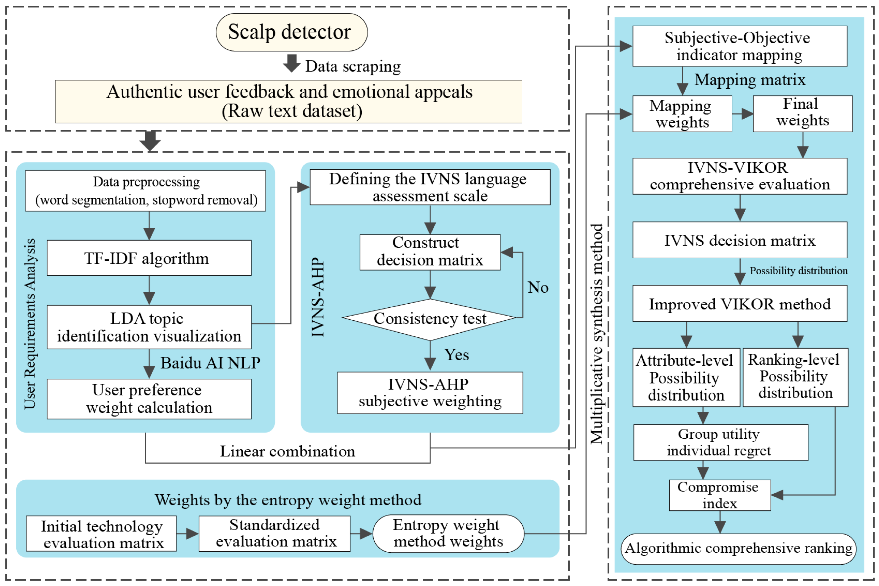
This paper aims to construct an improved decision model for the comprehensive evaluation of scalp detection algorithms, with the specific workflow illustrated in Figure 2. This model integrates IVNS theory, AHP, and VIKOR methodology. Its weighting system comprises subjective and objective components: First, NLP technology analyzes web-crawled user review text data to quantify user preferences, then determines composite subjective weights using the IVNS-AHP method. Second, employ EWM to calculate the objective weighting of technical metrics for target detection algorithms. Finally, the subjective and objective weights are multiplied to obtain the final weight. During the evaluation phase, based on the improved IVNS-VIKOR method, comprehensive ranking of algorithm solutions is achieved by calculating group utility, individual regret, and compromise indicators.

3.1. IVNS-AHP Subjective Empowerment

The IVNS-AHP procedure is as follows [34]:
Step 1. Identify objectives, criteria, and factors for the scheme-level study.
Step 2. Construct the IVNS language evaluation scale for AHP weight calculation, as shown in Table 1.
Step 3. Construct a pairwise comparison matrix using the IVNS language evaluation scale.
I V N S j i = I V N S i j C = F I V N S ij L , F I V N S ij U ,   1 I I V N S ij U , 1 I I V N S ij L ,   T I V N S ij L , T I V N S ij U
A ˜ I V N S = I V N S 11 I V N S 12 I V N S 1 n I V N S 21 I V N S 22 I V N S 2 n I V N S n 1 I V N S n 2 I V N S n n
If the importance of factor A i relative to B j is I V N S i j , The importance of B j relative to A i is determined by the symmetric equivalence class I V N S i j C . Additionally I V N S i i = 0.50 , 0.50 , 0.50 , 0.50 , 0.50 , 0.50 denotes the self-comparison item.
Step 4. The pairwise comparison matrix is deneutrosophicated using Equation (11) and subjected to a consistency check. If the deneutrosophicated pairwise comparison matrix passes the consistency test, then the consistency of the matrix constructed from the IVNS is considered to be validated.
CI = λ max n n 1
CR = CI RI
where n denotes the order of the matrix; CI represents the consistency index; CR denotes the consistency ratio; RI indicates the random consistency index.
Step 5. Normalize the IVNS matrix and calculate the arithmetic mean of each row to obtain the interval-valued neutrosophic weighting for the indicator.
I V N S i j = T i j L i = 1 n T i j U ,   T i j U i = 1 n T i j U ,   I i j L i = 1 n I i j U ,   I i j U i = 1 n I i j U ,   F i j L i = 1 n F i j U ,   F i j U i = 1 n F i j U
w j = i = 1 n I V N S i j n
Step 6. The weights are deneutrosophicated using Equation (11), and the IVNS-AHP weights w i AHP are obtained.
Step 7. Calculate the subjective weights using a linear combination approach, with the specific calculation method as follows:
w j s u b j = α w j u s e r + ( 1 α ) w j A H P
where w j s u b j denotes the composite subjective weight, α is set to 0.6 in this paper; see Section 5 for detailed discussion. w j u s e r represents the user preference weight, while w j A H P signifies the IVNS-AHP subjective weight.

3.2. Objective Weighting Using the EWM

The specific steps of the EWM are as follows:
Step 1. Let there be m scalp-detection algorithms and n technical indicators. Collect the objective performance data for each algorithm with respect to each indicator, and construct the initial technical evaluation matrix X ,
X = x 11 x 12 x 1 n x 21 x 22 x 2 n x m 1 x m 2 x m n
where x i j   represents the actual measurement value of the i-th algorithm on the j-th indicator.
Step 2. Standardize the data and construct the standardized evaluation matrix Y ,
y i j + = x i j min i ( x i j ) max i ( x i j ) min i ( x i j ) , i = 1 , 2 , , m , j = 1 , 2 , , n
y i j = max i ( x i j ) x i j max i ( x i j ) min i ( x i j ) , i = 1 , 2 , , m , j = 1 , 2 , , n
Y = ( y i j ) m × n , i = 1 , 2 , , m , j = 1 , 2 , , n
where y i j + denotes benefit-oriented indicators, y i j denotes cost-oriented indicators, and min i ( x i j ) represents the minimum value among all algorithms under the j-th indicator.
Step 3. Calculate the adjustment coefficient, the information entropy of each indicator, and the corresponding weights.
p i j = y i j k = 1 m y k j
H j = 1 ln m i = 1 m p i j ln ( p i j ) , j = 1 , 2 , n , H j 0
w j t e c h = 1 H j n k = 1 n H k
where p i j   denotes the normalization ratio, H j   represents information entropy, and w j t e c h indicates the objective weighting factor in the entropy weighting method.

3.3. Subjective-Objective Indicator Mapping

Due to the fuzziness and non-technical nature of user evaluation dimensions, it is difficult to establish a one-to-one correspondence with the quantifiable parameters observed during the actual operation of the algorithms. Therefore, a subjective–objective indicator mapping matrix needs to be constructed. Let the subjective indicator be denoted as P = p 1 , p 2 , p k and the objective indicator as Q = q 1 , q 2 , q m . Construct the subjective-objective indicator mapping matrix M = m i j k × n , where each element m i j represents the mapping strength of subjective indicator p i to objective indicator q j , i.e., the weight contribution. Thus, the mapping weight is
w j m a p = w j s u b j M
where w j m a p denotes the mapping weight, w j s u b j   represents the composite subjective weight, and M is the subjective-objective indicator mapping matrix.

3.4. Final Weighting of Indicators

This paper employs the multiplicative synthesis method to calculate the final weights of the indicators [35]:
w j f i n a l = w j m a p w j t e c h j = 1 n w j m a p w j t e c h
where w j f i n a l denotes the final weight, w j m a p denotes the mapping weight, and w j t e c h denotes the objective weight under the entropy weight method.

3.5. Improving the IVNS-VIKOR Comprehensive Evaluation

3.5.1. Constructing the IVNS Decision Matrix

Let the set of evaluation algorithms be A = A 1 , A 2 , A m , and the set of evaluation criteria be C = C 1 , C 2 , C n . An IVNS decision matrix X ~ = x i j m × n is constructed, where each evaluation value x i j   of algorithm A i under criterion C j is represented by an interval-valued neutrosophic number in the following form:
x ˜ i j = T i j L , T i j U , I i j L , I i j U , F i j L , F i j U
where T i j denotes the degree of acceptance of algorithm A i under criterion C j , I i j represents the degree of indeterminacy, and F i j represents the degree of falsity. According to the linguistic evaluation scale provided in Table 2, experts evaluate each algorithm, and the corresponding decision matrix is thereby constructed.

3.5.2. Determine the Positive and Negative Ideal Solutions

For benefit-type criteria, set the positive and negative ideal solutions as
x ˜ j + = T j + L , T j + U , I j + L , I j + U , F j + L , F j + U = max i T i j L ,   max i T i j U , min i I i j L , min i I i j U , min i F i j L , min i F i j U
x ˜ j = T j L , T j U , I j L , I j U , F j L , F j U = min i T i j L ,   min i T i j U , max i I i j L , max i I i j U , max i F i j L , max i F i j U
For cost-type criteria, set the positive and negative ideal solutions as
x ˜ j + = T j + L , T j + U , I j + L , I j + U , F j + L , F j + U = min i T i j L ,   min i T i j U , max i I i j L , max i I i j U , max i F i j L , max i F i j U
x ˜ j = T j L , T j U , I j L , I j U , F j L , F j U = max i T i j L ,   max i T i j U , min i I i j L , min i I i j U , min i F i j L , min i F i j U

3.5.3. Improved VIKOR Method

Inspired by reference [36], this paper extends the PD to the VIKOR method under the IVNS environment, and for the first time introduces an attribute-level possibility distribution (ALPD) based on the normalized difference in interval lengths. In addition, a ranking-level possibility distribution (RLPD) is defined to compare the possibility distributions of the compromise indicators, enabling finer-grained discrimination during the ranking stage. This improvement effectively enhances the model’s discriminative capability under approximate Q-value conditions and strengthens the precision and stability of the ranking results.
Step 1. Calculate the ALPD, defined by the following formula:
P ( x ˜ i j x ˜ j + ) = max 1 max γ j U + T i j L L ( x ˜ i j ) + L ( x ˜ j + ) ,   0 ,   0
γ j U + = T j U + + I j U + + F j U +
L ( x ˜ ) = ( T U T L ) + ( I U I L ) + ( F U F L )
where P ( x ~ i j x ~ j + ) represents the degree to which x ~ i j   is superior to the positive ideal solution, γ j U +   denotes the upper bound sum of the positive ideal solution interval, and L ( x ~ ) represents the length of the interval-valued neutrosophic number x ~ .
Step 2. Using the ALPD calculated in Step 1, compute the population utility S i and individual regret R i .
S i = j = 1 n w j f i n a l 1 ( P ( x ˜ i j x ˜ j + ) P min P max P min )
R i = max j w j f i n a l 1 ( P ( x ˜ i j x ˜ j + ) P min P max P min )
where w j f i n a l is the final weight of indicator C j . P m a x = m a x   P x ~ i j x ~ j + and P m i n = m i n   P x ~ i j x ~ j + represent the maximum and minimum possible values of all schemes under criterion C j , respectively.
Step 3. Integrate group utility and individual regret to calculate the compromise index Q i
Q i = v S i S min S max S min + ( 1 v ) R i R min R max R min
where v 0 , 1 is the decision mechanism coefficient, v is typically set to 0.5 to balance group utility and individual regret S m i n = m i n   S i , S m a x = m a x   S i .
Step 4. Calculate the RLPD, defined by the following formula:
P ( Q k Q l ) = max ( 0 , Q l U Q k L ) max ( 0 , Q k L Q l U ) ( Q k U Q k L ) + ( Q l U Q l L )
where P ( Q k Q l ) denotes the probability that algorithm   A k is not inferior to algorithm A l in a compromise sense. Q k L ,   Q k U ,   Q l L   and Q l U   represents the potential lower bound and upper bound of the compromise metric Q for algorithms A k   and A l , respectively.
Based on the RLPD P ( Q k Q l ) for every pair of alternatives, the evaluation algorithms are ultimately ranked according to P ( Q k Q l ) > 0.5 , and the ranking results are then aggregated. The formulas are as follows:
W k = l k 1 P ( Q k Q l ) > 0.5
P k = l k P ( Q k Q l )
where W k   denotes the number of pairwise comparisons won, and P k   represents the overall advantage score.

4. Empirical Research

4.1. User Requirement Weight Analysis

4.1.1. Data Sources and Preprocessing

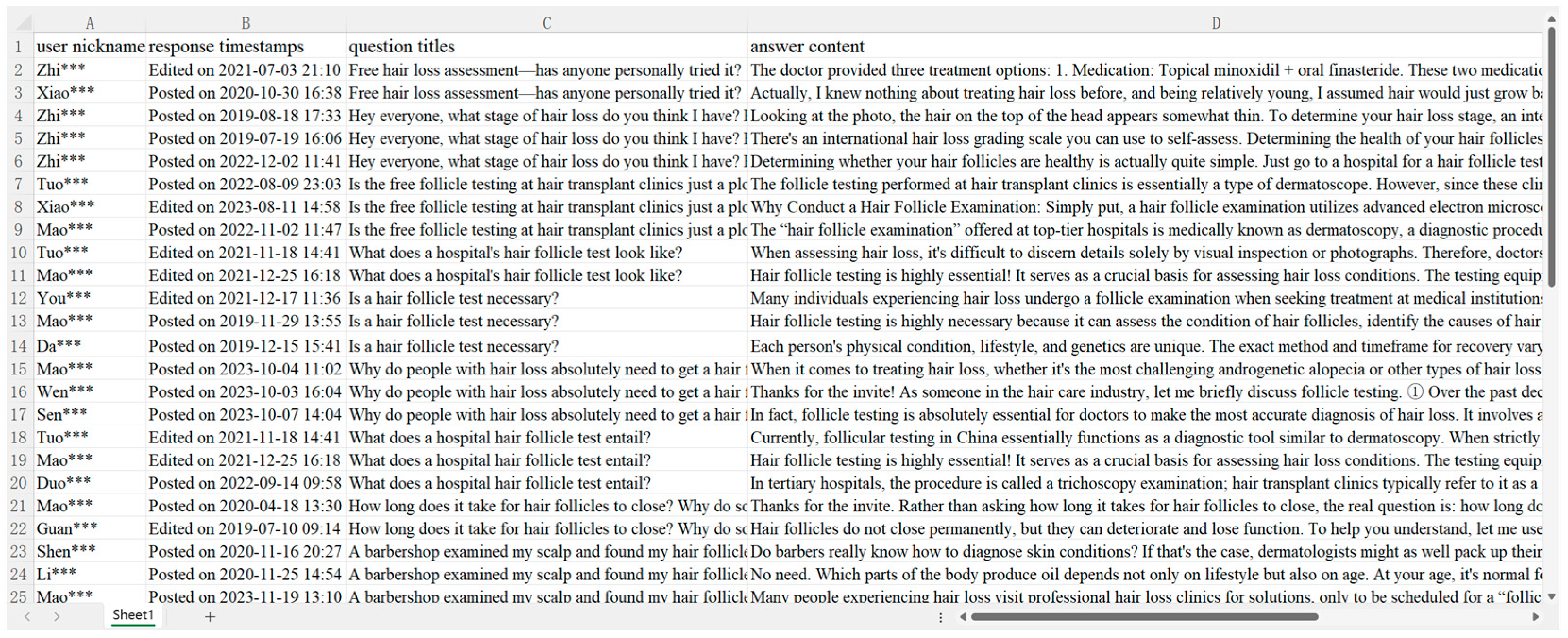
This paper utilized JD.com, Tmall, Xiaohongshu, and Weibo as data source platforms. Keywords such as “scalp analyzer,” “scalp health monitor,” and “scalp care device” were employed for retrieval. Data collection was conducted using the Octopus Web Scraper software (version 8.7.7), yielding a total of 169,341 text data entries. The exported initial comment dataset included user nicknames, response timestamps, question titles, and answer content, as shown in Figure 3.
The collected Chinese textual data were preprocessed through word segmentation and stop-word removal. Subsequently, the term frequencies and TF-IDF values of the segmented words were calculated according to Equations (1) and (2), as presented in Table 3.
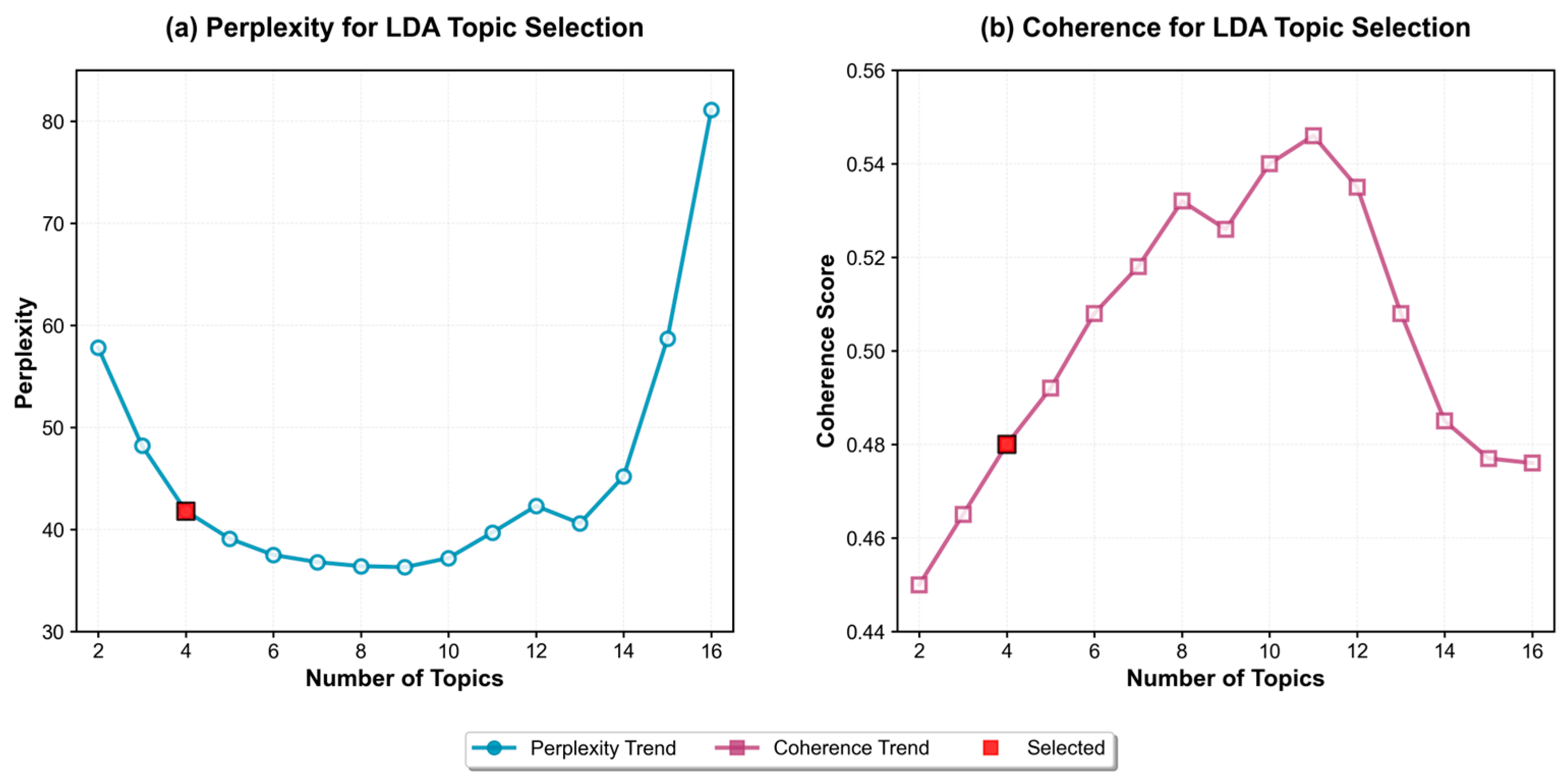
To address the issues of broad semantics and weak specificity in high-frequency vocabulary within review texts, this paper employs the LDA topic model for deep semantic modeling. Prior to model training, TF-IDF is applied to weight and optimize text features, significantly improving LDA’s topic clustering effectiveness and enhancing the model’s ability to capture deep semantics [37]. The number of topics was set between 2 and 16. According to Formulas (3) and (4), the corresponding confusion and consistency scores for each topic were calculated. A line chart illustrating the variation in perplexity/consistency scores with the number of topics is presented in Figure 4.
Based on the evaluation results, selecting four topics as the optimal number strikes a reasonable balance between model performance and practical application needs [38,39]. Although its perplexity (41.81) and coherence score (0.48) do not reach the theoretical optimum, this number of topics substantially reduces model complexity, greatly improves computational efficiency, and avoids the semantic fragmentation caused by excessive topic granularity.
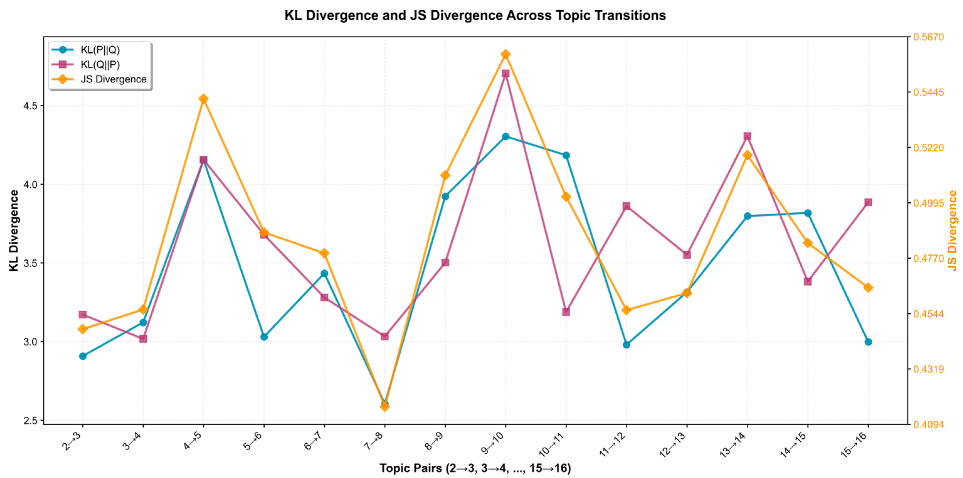
Inspired by [40], this paper further introduces Kullback–Leibler divergence (KLD) and Jensen–Shannon divergence (JSD) as auxiliary validation metrics to quantify the magnitude and stability of semantic structural changes under varying topic numbers. KLD measures the asymmetric difference between two probability distributions, whereas JSD, as its symmetric and smoothed extension, better captures the average semantic distance between topics, thereby reflecting changes in topic separability.
According to the divergence results between adjacent topic models (see Figure 5), when the number of topics increases from 3 to 4, the JSD rises to 0.4561, indicating enhanced semantic distinction and clearer topic boundaries. As the topic number further increases from 4 to 5, the JSD markedly rises to 0.5417, and the KLD (4.1548 and 4.1553) reach local peaks, suggesting that the model achieves its strongest semantic separation at this stage. This implies that four topics are sufficient to capture the dominant semantic space, and adding more topics may lead to excessive differentiation and redundant themes, thereby weakening overall interpretability.
In contrast, when the topic number increases from 5 to 6 and 6 to 7, the JSD slightly decreases (0.4874 and 0.4789), indicating a convergence of topic differences. At 7 to 8, the JSD further drops to 0.4166, implying that topic boundaries become blurred and model stability declines. Subsequently, during the 8 to 9 and 9 to 10 transitions, the JSD rises again, revealing a “semantic fluctuation–overlap” phenomenon, where newly generated topics partially overlap semantically with existing ones, thus reducing structural distinctiveness.
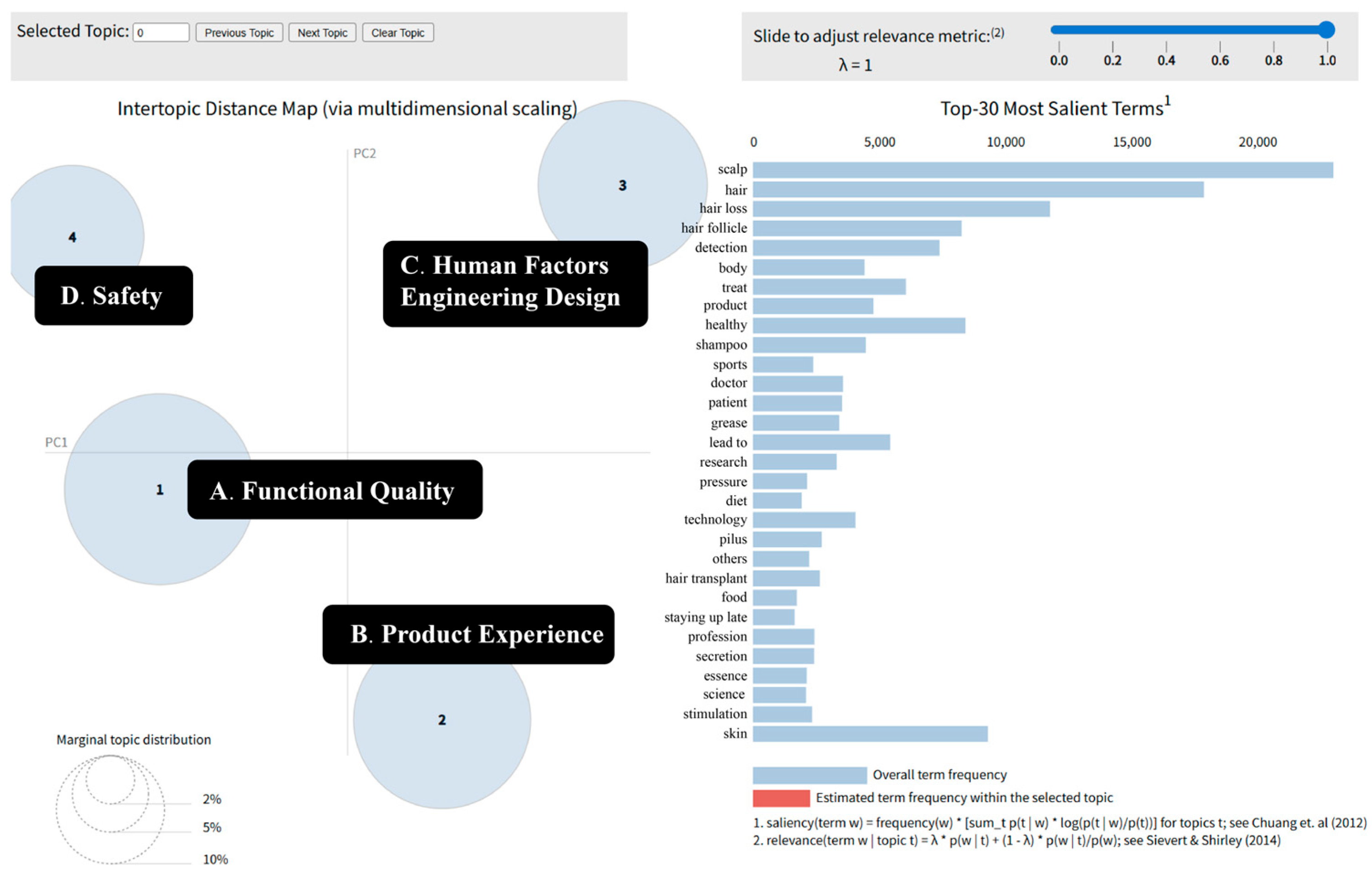
Based on the four themes identified from the preceding analysis, this paper employs the LDA topic modeling using the Gensim library (version 4.4.0) in Python (version 3.11) to analyze online text data. The visualization of the modeling results is implemented through the pyLDAvis library, and the topic clustering map is exported in HTML format (see Figure 6). In this visualization, each of the four bubbles represents a distinct topic, where the bubble size intuitively reflects the relative weight of that topic in the corpus, and the distance between bubbles quantifies the semantic similarity among topics—the closer the distance, the stronger the thematic correlation. The visualization results indicate that the LDA model achieves a clear and well-defined separation among topics.
This paper uses the LDA topic model to extract topics from online review texts and identifies four topic categories that reflect the needs of scalp detector users. The number of topics captures the multidimensional nature of user requirements, while the characteristic terms of each topic reveal its specific connotations. For each topic, we select the top 20 most frequent words as the core feature terms (see Table 4).
The four topics comprehensively characterize user requirements for scalp detectors from different dimensions:
(1)
Topic 1 “Functional Quality” focuses on product performance and reliability, covering core parameters such as resolution, accuracy, and stability to ensure that users’ expectations for detection outcomes are met.
(2)
Topic 2 “Product Experience” concerns the convenience of operational procedures and interface friendliness, including usability, intuitiveness, and after-sales service, which directly shape the overall user experience.
(3)
Topic 3 “Human Factors Engineering Design” delves into ergonomics and industrial design, involving adjustability convenience, tactile comfort, and multi-angle adaptability, balancing visual and haptic experiences.
(4)
Topic 4 “Safety” centers on user health and safety assurance, encompassing risk warnings and compliance measures, which constitute a critical prerequisite for product selection.
The four themes above serve as primary indicators. Based on theme-specific keywords, user requirements are further categorized as shown in Table 5, constituting the user requirement elements for the scalp detector discussed in this paper.

4.1.2. User Requirement Weight Calculation and Analysis

(1)
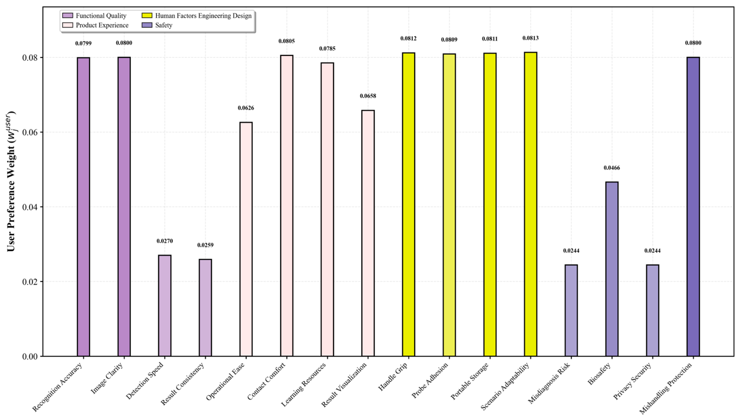
First, Algorithm 1 was used to call the Baidu Sentiment Analysis API to obtain sentiment polarity and confidence score results, as illustrated in Table 6. Finally, the user preference weights w j u s e r were calculated through normalization, and the results are shown in Figure 7.
(2)
IVNS-AHP Subjective Weighting
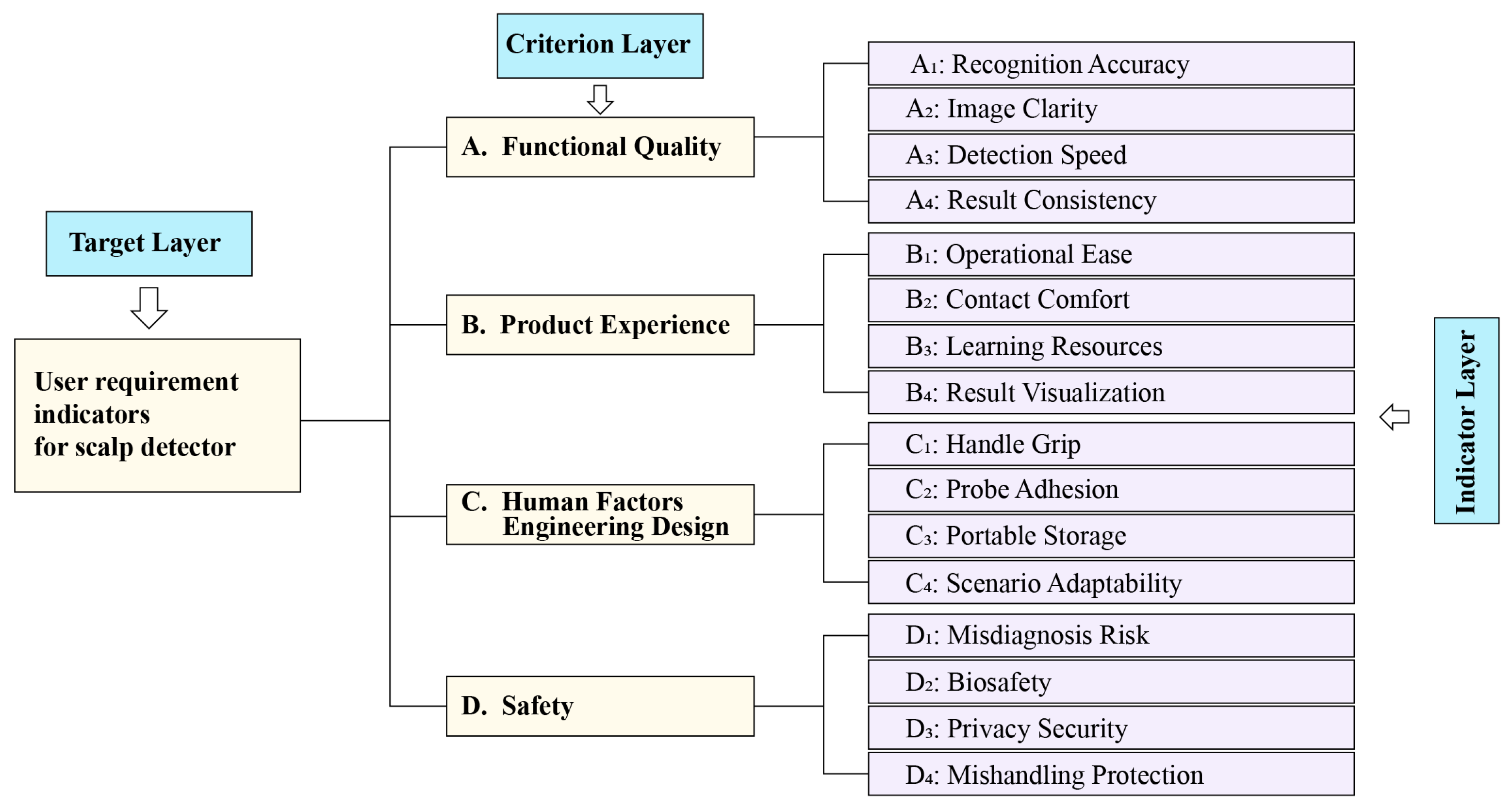
Based on text mining results from user reviews, this paper constructs a hierarchical model of user requirements for scalp detector, as shown in Figure 8.
To scientifically quantify the weighting of requirements at each level and construct an effective pairwise comparison matrix, this paper employs the Delphi Method to gather opinions from five domain experts and tenterminal user. The final results are presented in Table 7, Table 8, Table 9, Table 10 and Table 11. User requirement weights were derived using Equations (12)–(18), with the results shown in Table 12.

4.2. Experimental Design for Scalp

4.2.1. Experimental Environment and Parameter Configuration

This experiment was conducted on the Windows 10 Education operating system using Python 3.11.9, PyTorch 2.1.1, and CUDA 12.1. The hardware configuration is as follows: CPU: Intel® Core™ i9-9900K (Intel, Santa Clara, CA, USA); Memory: 64 GB DDR4 3200 MHz; Graphics Card: NVIDIA GeForce RTX 3060 (12 GB) (NVIDIA, Santa Clara, CA, USA).

4.2.2. Dataset Construction

This paper constructs a dataset dedicated to scalp inspection. Data acquisition was carried out using a specialized scalp detector jointly deployed with a partner client. The device is equipped with 50× and 200× optical lenses; at 50× magnification it can operate under three standard illumination modes (UV light, polarized light, and white light), enabling the capture of high-resolution scalp images under strictly controlled conditions. To ensure practical applicability, the images used in this paper come from scalp photos collected during the development of a scalp inspection system for the client. All acquisition procedures followed strict privacy protection protocols, and the images were de-identified after collection to ensure that no personally identifiable information is contained.
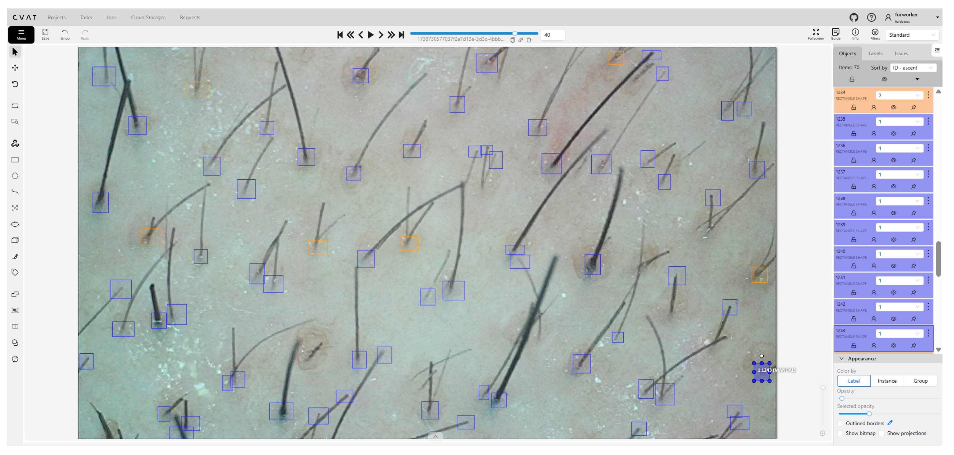
The original collection comprised 800 scalp images at 1920 × 1080 resolution. After quality screening, 28 blurred or strongly reflective images were removed, leaving 772 images. These were then cropped to 640 × 640 using a segmentation script, yielding a final dataset of 5035 images with 20,863 annotated instances. Annotation was conducted on a self-deployed CVAT platform on Tencent Cloud (see Figure 9). We defined three L0-level categories (singleroot, doubleroot, white-dandruff), with labeling performed by five annotators and reviewed by two experts. Inter-annotator agreement was assessed by randomly sampling 100 images for independent dual annotations at an IoU threshold of 0.5, resulting in an average IoU of 0.87 and a category agreement rate of 92.0%. The dataset was split into a training set with 2999 images and 12,343 instances, a validation set with 1044 images and 4440 instances, and a test set with 992 images and 4080 instances.

4.2.3. Algorithm Selection and Parameter Configuration

During the network training phase, to ensure experimental fairness and result reliability, this paper selected four representative object detection algorithms for comparative analysis. Training parameters were uniformly configured based on actual hardware environments. The algorithm selection and parameter settings are detailed in Table 13.
The evaluation algorithm encompasses the following performance metrics: Precision, Recall, mAP@0.5, F1 Score, FPS, and Parameters. The calculation formulas are as follows:
P r e c i s i o n = T P T P + F P × 100 %
R e c a l l = T P T P + F N × 100 %
m A P = 1 c k = 0 c A P k
where TP and FP represent the number of correctly predicted positive cases and incorrectly predicted positive cases, respectively; FN denotes the number of incorrectly predicted negative cases; APk is the average detection accuracy for the k-th category; c is the number of target categories.

4.2.4. Experimental Results

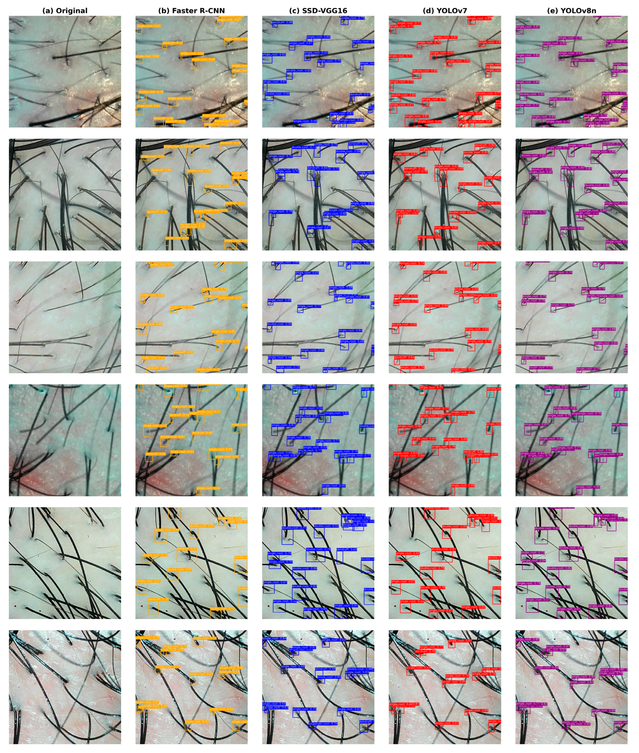
The performance comparison results of each algorithm are shown in Table 14. The detection results of different algorithms on the scalp detection dataset are illustrated in Figure 10.
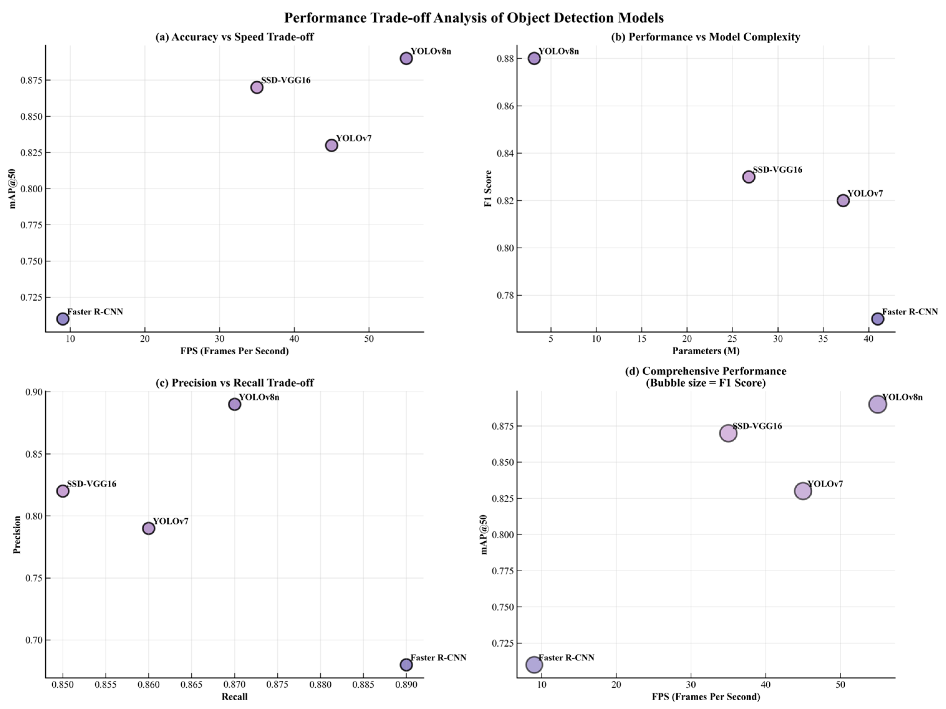
As shown in Figure 11, four subplots provide a multidimensional comparison of the algorithms in terms of accuracy, efficiency, and model complexity based on their performance on the self-built dataset. In the FPS–mAP@50 plot (a), YOLOv8n appears in the upper-right region, reflecting an excellent balance between detection accuracy and real-time capability. SSD-VGG16 also achieves relatively high precision with moderate speed, while Faster R-CNN remains in the lower-left quadrant due to its limited inference efficiency. In the Params–F1 Score plot (b), YOLOv8n attains the highest F1 score with the smallest parameter count, highlighting its lightweight yet effective architecture. SSD-VGG16 and YOLOv7 show moderate trade-offs between complexity and performance, whereas Faster R-CNN involves higher computational cost with relatively lower comprehensive accuracy. The Recall–Precision plot (c) indicates that SSD-VGG16 and YOLOv8n maintain a desirable equilibrium between detection completeness and correctness, while Faster R-CNN exhibits higher recall but lower precision, implying more false positives. The integrated bubble chart (d) further illustrates the distinct characteristics of each algorithm, with YOLOv8n showing a favorable combination of speed, precision, and overall balance under the experimental conditions. These results reveal the performance tendencies of different models on the customized dataset.

4.3. Final Weighting of Technical Indicators

4.3.1. Objective Weighting of Indicators via the EWM

Based on the experimental results and the calculations in Section 3.2 using Equations (19)–(25) the objective weights for each algorithm metric are determined, with the results presented in Table 15.

4.3.2. Computation of Subjective–Objective Indicator Mapping

To ensure the scientific rigor and applicability of the mapping matrix, we established the following principles after multiple in-depth consultations with domain experts: indicators that have a direct, linear relationship with technical metrics (e.g., recognition accuracy, detection speed) are directly mapped, with higher values assigned to stronger associations; for composite indicators, we decompose their intrinsic components and include only the parts that can be optimized by algorithms in the mapping, attributing the remaining parts to other R&D processes and marking them as N/A; indicators that depend entirely on hardware conditions, software frontend, or procedural specifications are excluded from algorithm evaluation, with their weights collectively marked as N/A. This approach ensures a clear evaluation scope and well-defined boundaries. The construction results of the mapping matrix are shown in Table 16.

4.3.3. Final Weight Calculation

Based on the preceding content and Equations (26) and (27), the final weights of the indicators are calculated as shown in Table 17.

4.4. Algorithmic Comprehensive Ranking

Improved VIKOR Method Calculation

Based on the VIKOR calculation method described in Section 3.5, five domain experts were again invited to score the technical indicators according to Table 2. The comprehensive results are presented in Table 18.
According to Equations (29)–(32), the positive and negative ideal solutions are determined, with results shown in Table 19. Based on the improved VIKOR method proposed in this paper and Equations (33)–(41), we compute the group utility, individual regret, and compromise index, and perform comparative ranking; the results are presented in Table 20.

5. Empirical Research Results Analysis

5.1. Sensitivity Analysis of the Parameter α in the Composite Subjective Weight

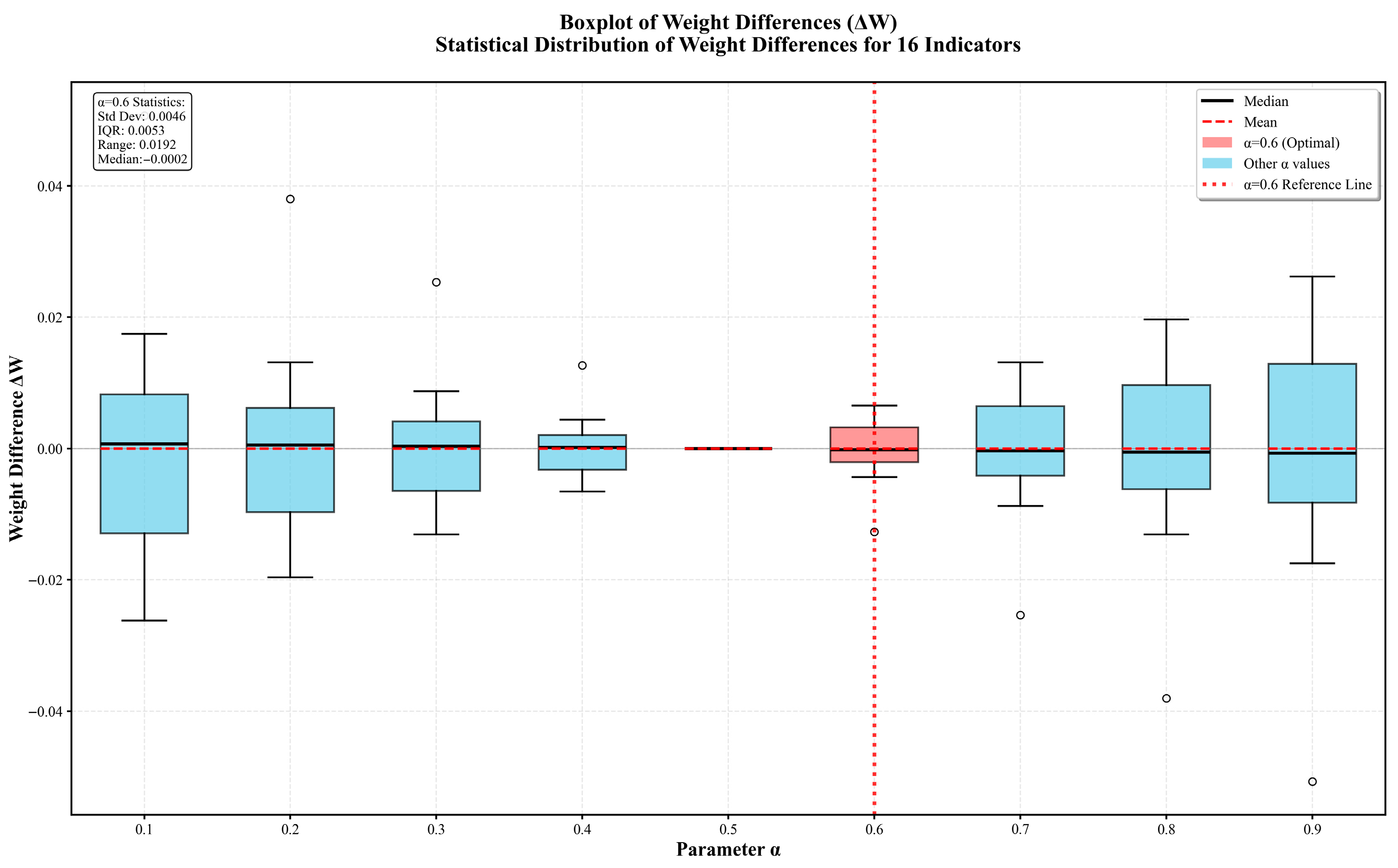
To validate the rationality of the parameter α in the composite subjective weight, this section systematically analyzes different values of α (see Figure 12).
The box plot illustrates the distribution of weight differences (ΔW) across the 16 secondary indicators under varying values of α. As α increases from 0.1 to 0.9, the model’s sensitivity to user preferences gradually strengthens. Within the range of α = 0.5–0.7, weight fluctuations are minimized, indicating good stability and robustness. Notably, at α = 0.5, the mean weight difference (ΔW) approaches zero, signifying that the weighting system achieves a balanced state between user preferences and expert judgment. This equilibrium point represents the stage where the decision process equally reflects subjective user orientation and expert analytical rationality.
At α = 0.6, the red box is markedly smaller than those at other α values, with the interquartile range (0.0053), standard deviation (0.0046), and range (0.0192) all reaching their minimums, while the median approaches zero (−0.0002). This indicates that the weight differences are most concentrated, exhibiting minimal fluctuations and the fewest outliers. Overall, the box plot presents a nearly symmetrical distribution centered around α = 0.5, confirming that the weight fusion mechanism maintains both structural balance and robustness. Accordingly, α = 0.6 is selected as the setting closest to this equilibrium point—slightly inclined toward user preferences—thereby aligning with the user-centered evaluation principle while preserving the rigor and stability of expert decision logic.
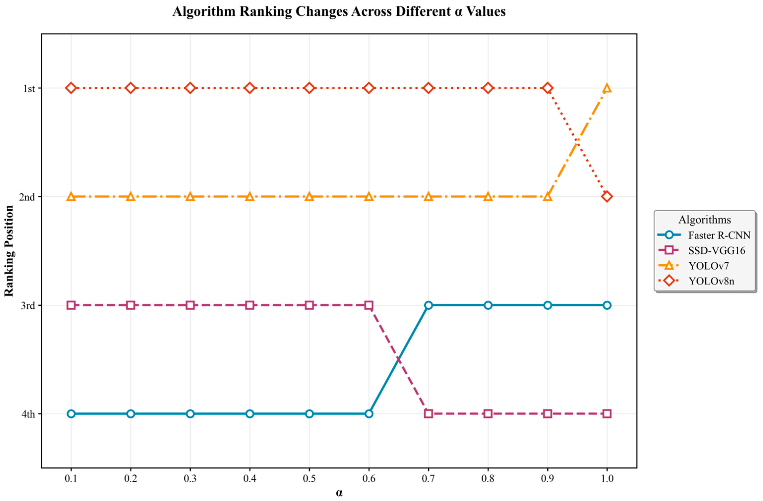
Furthermore, the ranking outcomes of the four detection algorithms under different values of α (see Figure 13) further validate the robustness of the proposed weighting mechanism. Within the range of α = 0.1–0.6, the ranking pattern remains completely consistent, with YOLOv8n and YOLOv7 continuously occupying the top two positions, followed by SSD-VGG16 and Faster R-CNN. As α increases to 0.7–0.9, only a minor exchange occurs between Faster R-CNN and SSD-VGG16 in the lower ranks, while the leading algorithms remain unchanged. When α reaches 1.0, YOLOv7 slightly surpasses YOLOv8n, reflecting the strengthened influence of expert weights.
This overall consistency across different α values demonstrates that the decision model is insensitive to moderate parameter variations, confirming that the fusion process effectively balances user-oriented and expert-driven perspectives. The stable ranking structure complements the box plot analysis, providing further evidence that α = 0.6 represents the most robust and interpretable configuration, achieving both internal equilibrium and practical decision stability.

5.2. Sensitivity Analysis of Preference Parameter v

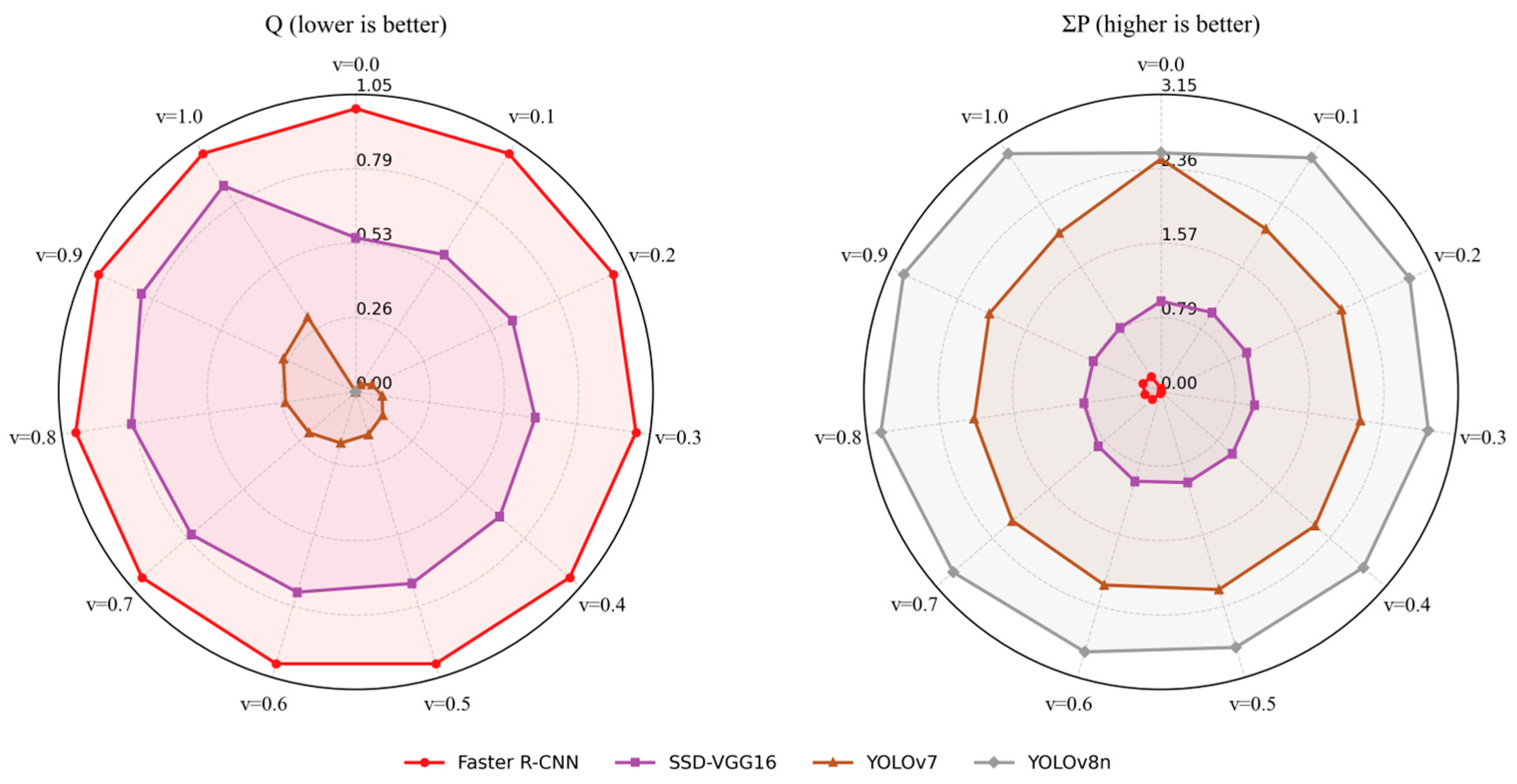
To examine the robustness of the decision results with respect to the preference parameter settings, a sensitivity analysis was conducted within the VIKOR framework for v∈{0, 0.1, 0.2, …, 1.00}, and the results are shown in Figure 14. The results indicate that the ranking of the models remains generally stable across different values of v, demonstrating good robustness of the decision outcomes.
YOLOv8n consistently exhibits the best overall performance under all v values, with the lowest Q values and overall advantage score ΣP that increases steadily from 2.5316 to 3.0000 as v grows. This trend suggests that the overall superiority of YOLOv8n further strengthens when greater weight is assigned to group utility in the decision process, securing its top-ranked position.
YOLOv7 maintains Q values close to, but slightly higher than, those of YOLOv8n. In some cases (e.g., v = 0), both models share identical Q values, yet YOLOv7 has a slightly lower ΣP (2.4684 vs. 2.5316). This indicates that although the two models have similar compromise levels, YOLOv8n achieves a higher overall advantage, enabling clearer differentiation in the rankings.
SSD-VGG 16 has Q values between those of YOLOv7 and Faster R-CNN, showing a steady increasing trend in both Q and ΣP (from 0.5441 to 0.8649 and from 0.9606 to 0.8066, respectively) as v increases. This reflects a certain degree of sensitivity to the parameter v; however, its overall advantage score remains higher than that of Faster R-CNN, keeping it in third place.
Faster R-CNN, with Q = 1.0000 under all parameter settings, exhibits the greatest deviation from the ideal solution. Meanwhile, its ΣP values are the lowest and show minimal fluctuation, indicating a clear disadvantage in terms of overall advantage.

5.3. Comparison with the Reference Method

This section aims to systematically compare the ranking performance of the proposed IVNS-AHP + EWM-VIKOR model with several representative approaches under the same evaluation dataset and indicator system (see Table 21). To ensure fairness and scientific validity of the comparison, all methods are implemented within an identical decision-making scenario and evaluated using the same indicator framework and dataset. The only differences lie in the procedures for weight determination, fuzzy information representation, and ranking algorithms.
Considering that the comparative methods are established under different fuzzy theoretical frameworks (such as IVNS, IVIF, IVPFN, TFN, FIS, and IF), this paper adopts a unified linguistic evaluation scale to convert the original data into fuzzy number representations compatible with each fuzzy environment, thereby ensuring semantic consistency of the information expressed across different methods. Moreover, the processes of fuzzy normalization, attribute weight integration, decision matrix construction, and defuzzification all follow uniform computational logic and operational principles, thereby minimizing the interference of non-model factors in the ranking results.
For models adopting a hybrid subjective–objective weighting scheme, the ratio coefficient between the two sources of information was fixed to a unified value to ensure comparability of weight allocation under consistent parameter settings. For methods relying solely on either subjective or objective weighting, normalization procedures were applied to standardize the weight vectors, ensuring scale consistency across all compared approaches.
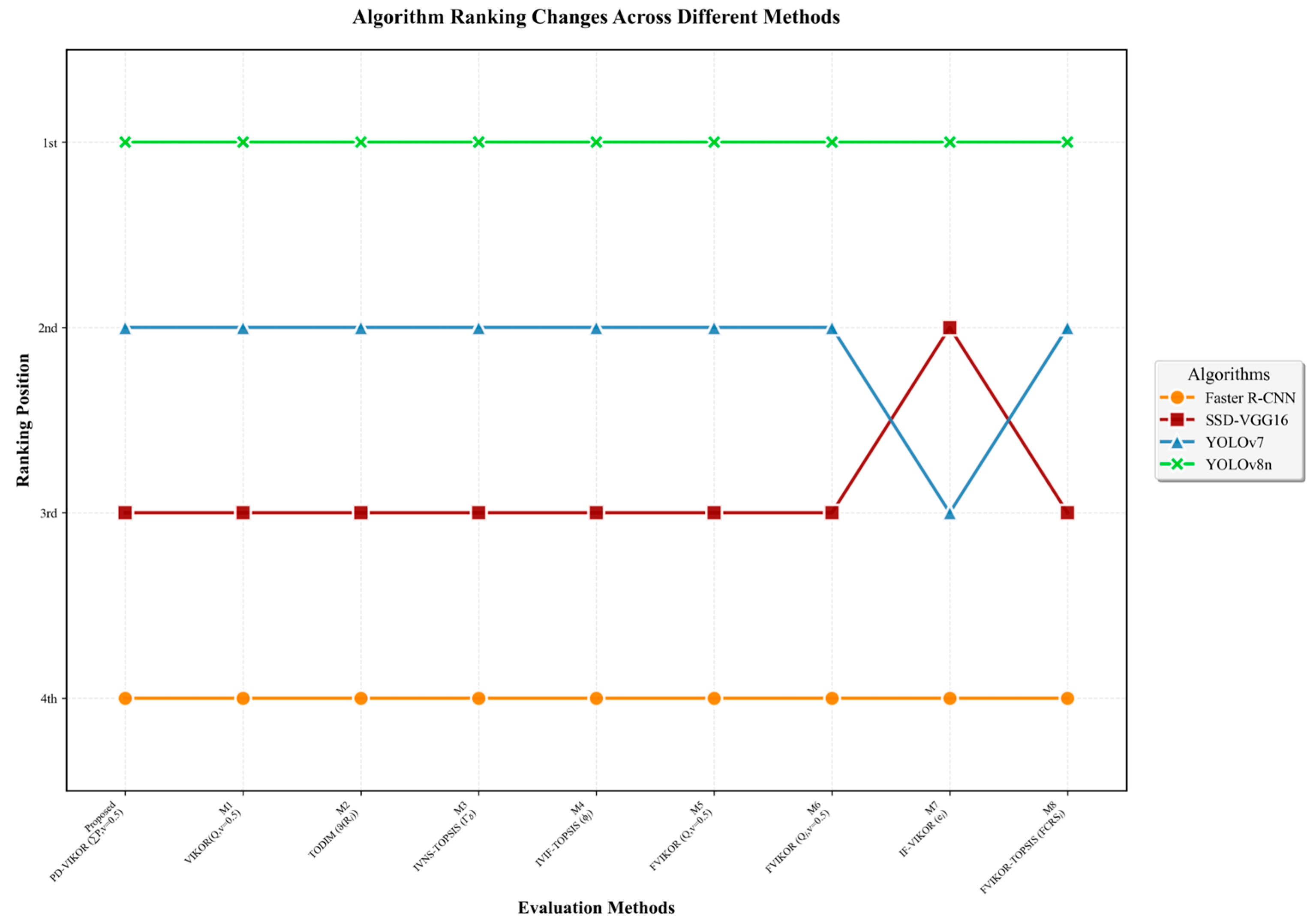
In the comparative experiments, the proposed PD-VIKOR approach demonstrates superior ranking precision and discrimination capability in evaluating four target detection algorithms. By integrating both the Q value and the overall preference degree (ΣP), the PD-VIKOR method effectively avoids the ranking ambiguity commonly observed in traditional VIKOR models under extreme parameter settings, while enhancing the differentiation between alternatives. In this experiment, YOLOv8n consistently ranks first and Faster R-CNN last across all methods, indicating a stable consensus in the ranking trend of mainstream models when evaluated from multiple dimensions, including user experience, detection accuracy, and computational efficiency (see Table 22).
It is noteworthy that in the M1 method with v = 0, the Q values of models 1 and 2 are both equal to zero, resulting in an inability to effectively distinguish between them. This finding highlights the inherent risk of ranking failure in the traditional VIKOR approach when boundary parameters are applied. In contrast, the proposed PD-VIKOR method introduces the comprehensive superiority degree (ΣP) as a supplementary criterion, enabling effective discrimination even when Q values are identical or extremely close. This enhancement not only improves ranking robustness and interpretability but also extends the applicability of VIKOR to uncertain and imprecise decision-making contexts.
Additionally, the M7 method produces an inconsistent ranking order of “4 ≻ 2 ≻ 3 ≻ 1” (see Figure 15), where SSD-VGG16 outranks YOLOv7, which contradicts their respective scores (0.5784 vs. 0.6452) and the results obtained by most other methods. This inconsistency indicates that M7 is sensitive to minor score differences, potentially influenced by the definition of the fuzzy distance measure or the distribution of score intervals, leading to instability in ranking direction. In contrast, the PD-VIKOR approach maintains a consistent ranking structure under the same dataset, demonstrating stronger ranking stability and result reliability.

6. Conclusions and Future Work

This paper extends the AHP-VIKOR fusion method to IVNS, introduces the PD to improve the VIKOR method, and conducts an empirical analysis of mainstream algorithms using mAP@50, Precision, Recall, F1 Score, FPS and Params as evaluation indicators. The main findings are as follows:
First, this paper combines subjective user preferences extracted through NLP and IVNS–AHP with objective weights derived from the EWM, forming a method for determining fusion weights guided by user perception. The weight coefficient α = 0.6 emphasizes the dominant role of user preferences. At the same time, objective weights constrain and modify the evaluation process, enabling the model to achieve an optimal balance between user experience and data consistency.
Second, in the IVNS environment, the proposed PD-VIKOR method maintains consistent rankings under various preference parameters, demonstrating excellent robustness and sensitivity control. In particular, when Q values are close, the overall dominance ΣP can more accurately capture subtle performance differences between models, thereby improving the resolution and credibility of the ranking results.
Finally, ccross-method validation using TODIM, TOPSIS, and their fuzzy extensions (IVNS-TOPSIS, IVIF-TOPSIS, FVIKOR-TOPSIS) reveals strong consistency in ranking performance, with most methods converging on the order “4 ≻ 3 ≻ 2 ≻ 1”. This convergence not only underscores the theoretical soundness of the perception-based evaluation but also provides empirical evidence supporting the effectiveness of the integrated subjective–objective weighting system.
This paper provides practical guidance for algorithm selection and engineering implementation. In decision-making scenarios that integrate multidimensional performance metrics and user perception, the proposed model effectively assists the R&D team in balancing algorithmic accuracy, processing speed, and resource consumption, thereby offering a scientific basis for selecting the optimal algorithm in the practical deployment of scalp detection devices.
Future studies will focus on further improving data reliability, model adaptability, and interdisciplinary applicability. First, to mitigate potential bias and noise in e-commerce user reviews, future work will employ large language models for deeper semantic understanding, sentiment disambiguation, and context-aware filtering, thereby capturing user intent more accurately and reducing the impact of group bias and linguistic ambiguity. Second, as the current IVNS scale and interval settings depend on expert prior knowledge, subsequent research will explore adaptive and self-learning weighting mechanisms to dynamically adjust membership functions and possibility distributions according to evolving data characteristics. Third, longitudinal analyses and temporal evolution models can be introduced to capture the dynamic nature of user preferences and algorithm performance over time, enabling a more comprehensive understanding of the model’s stability and adaptability. Furthermore, expanding the framework to multi-language and cross-cultural datasets will be considered to examine its generalizability and cultural robustness. In addition, future work will consider integrating the proposed methodology into modular Python scripts to facilitate automated implementation and enhance practical scalability. Finally, the proposed perception-driven decision-making framework can be extended to other intelligent product domains to validate its generalizability and strengthen its role as a human-centered decision-support tool in complex engineering environments.

Author Contributions

Conceptualization: X.C., R.Z. and W.S.; Methodology: X.C. and R.Z.; Software: X.C.; Validation: X.C., R.Z. and W.S.; Formal analysis: X.C.; Investigation: X.C.; Resources: R.Z. and W.S.; Data curation: X.C.; Writing—original draft: X.C.; Writing—review and editing: R.Z. and W.S.; Visualization: X.C.; Supervision: R.Z. and W.S.; Project administration: R.Z.; Funding acquisition: R.Z. All authors have read and agreed to the published version of the manuscript.

Funding

This work was supported by the Guangzhou Civil Affairs Science and Technology Fund Project: Challenge-Based Technical Breakthrough Initiative (grant no. GCAAL2022001); the Guangzhou Key R&D Program (grant nos. 2023B04J0106 and 2023B04J0121); and the Ministry of Education Humanities and Social Sciences Research Planning Fund (grant no. 23YJAZH201).

Institutional Review Board Statement

Not applicable.

Informed Consent Statement

Not applicable.

Data Availability Statement

The original contributions presented in this study are included in the article. Further inquiries can be directed to the corresponding author.

Conflicts of Interest

The authors declare no conflicts of interest.

Abbreviations

The following abbreviations are used in this manuscript:
MAGDMmulti-attribute group decision-making
IVNSinterval-valued neutrosophic set
AHPanalytic hierarchy process
NLPnatural language processing
EWMentropy weight method
VIKORVlse Kriterijumska Optimizacija Kompromisno Resenje
PDpossibility distribution
KLDKullback–Leibler divergence
JSDJensen–Shannon divergence
mAP@50mean Average Precision at IoU = 0.5
FPSframes per second
TODIMan acronym in Portuguese of interactive and multiple attribute decision-making
TOPSISTechnique for Order Preference by Similarity to an Ideal Solution
C-IFcircular intuitionistic fuzzy
IVq-ROFSinterval-valued q-rung orthopair fuzzy set
TFterm frequency
TF-IDFterm frequency-inverse document frequency
LDALatent Dirichlet Allocation
ALPDattribute-level possibility distribution
RLPDranking-level possibility distribution

References

  1. Wu, X.; Chen, D.; Xun, F.; Zhang, M.; Tang, X. Developingrehabilitation services to promote the achievement of the “Healthy China 2030”goals. Chin. J. Rehabil. Theory Pract. 2022, 28, 6–14. (In Chinese) [Google Scholar]
  2. Mathias, R.; McCulloch, P.; Chalkidou, A.; Gilbert, S. Digital Health Technologies Need Regulation and Reimbursement That Enable Flexible Interactions and Groupings. Npj Digit. Med. 2024, 7, 148. [Google Scholar] [CrossRef]
  3. Garg, V. Wearable Wisdom: How AI-Powered Devices Are Driving Personalized Preventive Care. World J. Adv. Eng. Technol. Sci. 2025, 15, 196–206. [Google Scholar] [CrossRef]
  4. Li, H.; Wang, Y.; Zhang, Q.; Yu, S.S.; Wang, F.; Chen, S.; Lim, C.P. Dynamic Personalized Health Management through the Health Assistant AI Fusion Framework. Inf. Fusion 2025, 123, 103263. [Google Scholar] [CrossRef]
  5. Maleki Varnosfaderani, S.; Forouzanfar, M. The Role of AI in Hospitals and Clinics: Transforming Healthcare in the 21st Century. Bioengineering 2024, 11, 337. [Google Scholar] [CrossRef]
  6. Pang, K.; Fu, C.; Martínez, L.; Liu, J.; Zou, L.; Lu, M. An Extended Multi-Expert Concept Lattice-Based Heterogeneous Multi-Attribute Group Decision-Making Approach. Inf. Sci. 2024, 665, 120345. [Google Scholar] [CrossRef]
  7. Wang, Y.; Zhan, J.; Zhang, C.; Xu, Z. A Group Consensus Model with Prospect Theory under Probabilistic Linguistic Term Sets. Inf. Sci. 2024, 653, 119800. [Google Scholar] [CrossRef]
  8. Sahoo, S.K.; Goswami, S.S. A ComprehensiveReview of Multiple Criteria Decision-Making (MCDM) Methods: Advancements, Applications, and Future Directions. Decis. Mak. Adv. 2023, 1, 25–48. [Google Scholar] [CrossRef]
  9. Chaibate, H.; Hadek, A.; Ajana, S.; Bakkali, S. Analytical Hierarchy Process Applied to Pedagogical Method Selection Problems. Educ. Res. Int. 2021, 2021, 6664758. [Google Scholar] [CrossRef]
  10. Srdjevic, B.; Srdjevic, Z.; Reynolds, K.M.; Lakicevic, M.; Zdero, S. Using Analytic Hierarchy Process and Best–Worst Method in Group Evaluation of Urban Park Quality. Forests 2022, 13, 290. [Google Scholar] [CrossRef]
  11. Jabreel, M.; Maaroof, N.; Valls, A.; Moreno, A. Introducing Sentiment Analysis of Textual Reviews in a Multi-Criteria Decision Aid System. Appl. Sci. 2020, 11, 216. [Google Scholar] [CrossRef]
  12. Zheng, J.; Wang, S.; Wang, Z. Circular Pythagorean Fuzzy Deck of Cards Model for Optimal Deep Learning Architecture in Media Sentiment Interpretation. Symmetry 2025, 17, 1399. [Google Scholar] [CrossRef]
  13. Yadav, S.; Kaur, G.; Kapur, P.K.; Aggarwal, A.G. Intuitionistic Fuzzy and Multi-Criteria Based Ranking of Mobile Payment Apps Using Sentiment Score of Online Reviews. Int. J. Syst. Assur. Eng. Manag. 2024, 15, 1–14. [Google Scholar] [CrossRef]
  14. Xu, M.; Wang, X.; Xu, Z. Tour Group Prioritization Driven by Online Reviews: Using an Improved EDAS-SIR Method with Credibility. Artif. Intell. Rev. 2025, 58, 77. [Google Scholar] [CrossRef]
  15. Roszkowska, E.; Filipowicz-Chomko, M. Airline Ranking Using Social Feedback and Adapted Fuzzy Belief TOPSIS. Entropy 2025, 27, 879. [Google Scholar] [CrossRef]
  16. Zhang, C.; Tian, Y.; Fan, L.; Li, Y. Customized Ranking for Products through Online Reviews: A Method Incorporating Prospect Theory with an Improved VIKOR. Appl. Intell. 2020, 50, 1725–1744. [Google Scholar] [CrossRef]
  17. Alamoodi, A.H.; Mohammed, R.T.; Albahri, O.S.; Qahtan, S.; Zaidan, A.A.; Alsattar, H.A.; Albahri, A.S.; Aickelin, U.; Zaidan, B.B.; Baqer, M.J.; et al. Based on Neutrosophic Fuzzy Environment: A New Development of FWZIC and FDOSM for Benchmarking Smart e-Tourism Applications. Complex Intell. Syst. 2022, 8, 3479–3503. [Google Scholar] [CrossRef]
  18. Smarandache, F. A Unifying Field in Logics: Neutrosophic Logic: Neutrosophy, Neutrosophic Set, Neutrosophic Probability and Statistics, 4th ed.; American Research Press: Rehoboth, DE, USA, 1998; ISBN 978-1-59973-080-6. [Google Scholar]
  19. Zhang, H.; Wang, L. The Service Quality Evaluation of Agricultural E-Commerce Based on Interval-Valued Intuitionistic Fuzzy GRA Method. J. Math. 2022, 2022, 3931136. [Google Scholar] [CrossRef]
  20. Liu, S.; Yu, W.; Chan, F.T.S.; Niu, B. A Variable Weight-based Hybrid Approach for Multi-attribute Group Decision Making under Interval-valued Intuitionistic Fuzzy Sets. Int. J. Intell. Syst. 2021, 36, 1015–1052. [Google Scholar] [CrossRef]
  21. Zhou, Y.; Zhang, X.; Chen, Y.; Xu, X.; Li, M. A Water-Land-Energy-Carbon Nexus Evaluation of Agricultural Sustainability under Multiple Uncertainties: The Application of a Multi-Attribute Group Decision Method Determined by an Interval-Valued Intuitionistic Fuzzy Set. Expert Syst. Appl. 2024, 242, 122833. [Google Scholar] [CrossRef]
  22. Wang, J.-C.; Chen, T.-Y. A Compromise Decision-Support Technique with an Augmented Scoring Function within Circular Intuitionistic Fuzzy Settings. Eng. Appl. Artif. Intell. 2024, 128, 107359. [Google Scholar] [CrossRef]
  23. Hendiani, S.; Walther, G. Double-Layer Multi-Criteria Group Decision-Making Approach Using Neutralized Possibility Degree-Based Decision Matrix with Fuzzy Information. Eng. Appl. Artif. Intell. 2024, 133, 108276. [Google Scholar] [CrossRef]
  24. Chen, T.-Y. An Advanced Approach to Multiple Criteria Optimization and Compromise Solutions under Circular Intuitionistic Fuzzy Uncertainty. Adv. Eng. Inform. 2023, 57, 102112. [Google Scholar] [CrossRef]
  25. Mustafa, Z.; Amin, R.; Aldabbas, H.; Ahmed, N. Intrusion Detection Systems for Software-Defined Networks: A Comprehensive Study on Machine Learning-Based Techniques. Clust. Comput. 2024, 27, 9635–9661. [Google Scholar] [CrossRef]
  26. Zhou, Y.-J.; Zhou, M.; Yang, J.-B.; Cheng, B.-Y.; Wu, J. Decentralized Multipartite Consensus Model for Multi-Attribute Group Decision Making: A User Experience-Oriented Perspective. Expert Syst. Appl. 2025, 287, 127917. [Google Scholar] [CrossRef]
  27. Chen, T.; Peng, L.; Yang, J.; Cong, G. Analysis of User Needs on Downloading Behavior of English Vocabulary APPs Based on Data Mining for Online Comments. Mathematics 2021, 9, 1341. [Google Scholar] [CrossRef]
  28. Fang, B.; Hu, E.; Shen, J.; Zhang, J.; Chen, Y. Implicit Feedback Recommendation Method Based on User-Generated Content. Sci. Program. 2021, 2021, 3982270. [Google Scholar] [CrossRef]
  29. Blei, D.M.; Ng, A.Y.; Jordan, M.I. Latent Dirichlet Allocation. J. Mach. Learn. Res. 2003, 3, 993–1022. [Google Scholar]
  30. Wu, H.; Yi, H.; Li, C. An Integrated Approach for Detecting and Quantifying the Topic Evolutions of Patent Technology: A Case Study on Graphene Field. Scientometrics 2021, 126, 6301–6321. [Google Scholar] [CrossRef]
  31. Sharma, A.; Rana, N.P.; Nunkoo, R. Fifty Years of Information Management Research: A Conceptual Structure Analysis Using Structural Topic Modeling. Int. J. Inf. Manag. 2021, 58, 102316. [Google Scholar] [CrossRef]
  32. Broumi, S.; Talea, M.; Bakali, A.; Smarandache, F.; Nagarajan, D.; Lathamaheswari, M.; Parimala, M. Shortest Path Problem in Fuzzy, Intuitionistic Fuzzy and Neutrosophic Environment: An Overview. Complex Intell. Syst. 2019, 5, 371–378. [Google Scholar] [CrossRef]
  33. Alioğulları, E.; Türkan, Y.S.; Çakmak, E.; Tirkolaee, E.B. Evaluation of Risk Strategies for Supply Chain Sustainability with Interval-Valued Neutrosophic Fuzzy EDAS. Heliyon 2024, 10, e38607. [Google Scholar] [CrossRef]
  34. Bolturk, E.; Kahraman, C. A Novel Interval-Valued Neutrosophic AHP with Cosine Similarity Measure. Soft Comput. 2018, 22, 4941–4958. [Google Scholar] [CrossRef]
  35. Chen, C.-H. A Novel Multi-Criteria Decision-Making Model for Building Material Supplier Selection Based on Entropy-AHP Weighted TOPSIS. Entropy 2020, 22, 259. [Google Scholar] [CrossRef]
  36. Garg, H. A New Possibility Degree Measure for Interval-valued Q-rung Orthopair Fuzzy Sets in Decision-making. Int. J. Intell. Syst. 2021, 36, 526–557. [Google Scholar] [CrossRef]
  37. Bala, S.; Kumari, S. Comprehensive Analysis of Variants of TF-IDF Applied on LDA and LSA Topic Modelling. Int. J. Eng. Adv. Technol. 2020, 9, 531–535. [Google Scholar] [CrossRef]
  38. Koczkodaj, W.W.; Nowacki, M.; Pedrycz, W.; Strzalka, D. Text Mining Analysis of over 392 Million Compromised Healthcare Records. Adv. Sci. Technol. Res. J. 2024, 19, 73–81. [Google Scholar] [CrossRef]
  39. Rahman, M.; Frame, J.M.; Lin, J.; Nearing, G.S. Hydrology Research Articles Are Becoming More Topically Diverse. J. Hydrol. 2022, 614, 128551. [Google Scholar] [CrossRef]
  40. Cao, Y.; Zhang, Y.; Shi, Y.; Ren, Y. From Policy to Practice: A Comparative Topic Modeling Study of Smart Forestry in China. Forests 2025, 16, 1019. [Google Scholar] [CrossRef]
  41. Chuang, J.; Manning, C.D.; Heer, J. Termite: Visualization Techniques for Assessing Textual Topic Models. In Proceedings of the International Working Conference on Advanced Visual Interfaces, Capri Island, Italy, 21–25 May 2012; pp. 74–77. [Google Scholar] [CrossRef]
  42. Sievert, C.; Shirley, K. LDAvis: A Method for Visualizing and Interpreting Topics. In Proceedings of the Workshop on Interactive Language Learning, Visualization, and Interfaces, Baltimore, MD, USA, 27 June 2014; Association for Computational Linguistics; pp. 63–70. [Google Scholar] [CrossRef]
  43. Girshick, R. Fast R-CNN. In Proceedings of the 2015 IEEE International Conference on Computer Vision (ICCV), Santiago, Chile, 7–13 December 2015; IEEE: Piscataway, NJ, USA, 2015; pp. 1440–1448. [Google Scholar] [CrossRef]
  44. Kang, H.-J. Real-Time Object Detection on640x480 Image with VGG16+SSD. In Proceedings of the 2019 International Conference on Field-Programmable Technology (ICFPT), Tianjin, China, 9–13 December 2019; IEEE: Piscataway, NJ, USA, 2019; pp. 419–422. [Google Scholar] [CrossRef]
  45. Chen, T.; Li, H.; Chen, J.; Zeng, Z.; Han, C.; Wu, W. Detection Network for Multi-Size and Multi-Target Tea Bud Leaves in the Field of View via Improved YOLOv7. Comput. Electron. Agric. 2024, 218, 108700. [Google Scholar] [CrossRef]
  46. Liu, J.; Zhang, B.; Xu, H.; Zhang, L.; Zhang, X. Method for Recognizing Disordered Sugarcane Stacking Based on Improved YOLOv8n. Appl. Sci. 2024, 14, 11765. [Google Scholar] [CrossRef]
  47. Yu, Y.; Zutty, J. LLM-Guided Evolution: AnAutonomous Model Optimization for Object Detection. In Proceedings of the Genetic and Evolutionary Computation Conference Companion (GECCO’25 Companion), Málaga, Spain, 14–18 July 2025; ACM: New York, NY, USA, 2025; pp. 2363–2370. [Google Scholar] [CrossRef]
  48. Fränti, P.; Mariescu-Istodor, R. Soft Precision and Recall. Pattern Recognit. Lett. 2023, 167, 115–121. [Google Scholar] [CrossRef]
  49. Huynh, N.; Nguyen, K.-D. Real-Time Droplet Detection for Agricultural Spraying Systems: A Deep Learning Approach. Mach. Learn. Knowl. Extr. 2024, 6, 259–282. [Google Scholar] [CrossRef]
  50. Zhang, J. Evolution of YOLO: A Comparative Analysis of YOLOv5, YOLOv8, and YOLOv10. Appl. Comput. Eng. 2025, 119, 173–181. [Google Scholar] [CrossRef]
  51. Zhang, Y.; Song, J.; Yu, X.; Ji, X. WMC-RTDETR: A Lightweight Tea Disease Detection Model. Front. Plant Sci. 2025, 16, 1574920. [Google Scholar] [CrossRef]
  52. Zhang, J.; Zhang, Y.; Zhou, J. Research on Lightweight Infrared Target Detection Algorithm Based on Deep Learning. Eng. Lett. 2025, 33, 2589. [Google Scholar]
  53. Fan, J.; Li, D.; Wu, M. An Extended TODIM Method with Unknown Weight Information Under Interval-Valued Neutrosophic Environment for FMEA. Int. J. Comput. Intell. Syst. 2020, 14, 174. [Google Scholar] [CrossRef]
  54. Tam, P.M.; Hang, D.T.; Thuy, P.T.; Dat, L.Q. Comprehensive Evaluation of Sustainable Consumption towards Green Growth Based on an Interval Valued Neutrosophic TOPSIS Approach. Environ. Sci. Pollut. Res. 2023, 30, 89838–89858. [Google Scholar] [CrossRef]
  55. Yildiz, A.; Guneri, A.F.; Ozkan, C.; Ayyildiz, E.; Taskin, A. An Integrated Interval-Valued Intuitionistic Fuzzy AHP-TOPSIS Methodology to Determine the Safest Route for Cash in Transit Operations: A Real Case in Istanbul. Neural Comput. Appl. 2022, 34, 15673–15688. [Google Scholar] [CrossRef]
  56. Demir, E.; Ak, M.F.; Sarı, K. Pythagorean Fuzzy Based AHP-VIKOR Integration to Assess Rail Transportation Systems in Turkey. Int. J. Fuzzy Syst. 2023, 25, 620–632. [Google Scholar] [CrossRef]
  57. Das, A.; Kumar, V.; Dutta, S. A Fuzzy-Based AHP-VIKOR Framework for Risk Analysis of Safety-Critical Systems: A Case Study of Nuclear Power Plant. Ann. Nucl. Energy 2024, 209, 110841. [Google Scholar] [CrossRef]
  58. Tripathi, D.K.; Nigam, S.K.; Cavallaro, F.; Rani, P.; Mishra, A.R.; Hezam, I.M. A Novel CRITIC-RS-VIKOR Group Method with Intuitionistic Fuzzy Information for Renewable Energy Sources Assessment. Group Decis. Negot. 2023, 32, 1437–1468. [Google Scholar] [CrossRef]
  59. Sarıkaya, H.A. A Hybrid MCDM Model for Personnel Evaluation: Integrating AHP, Fuzzy TOPSIS and VIKOR with Composite Scoring. J. Appl. Eng. Agric. 2025, 2, 44–71. [Google Scholar]
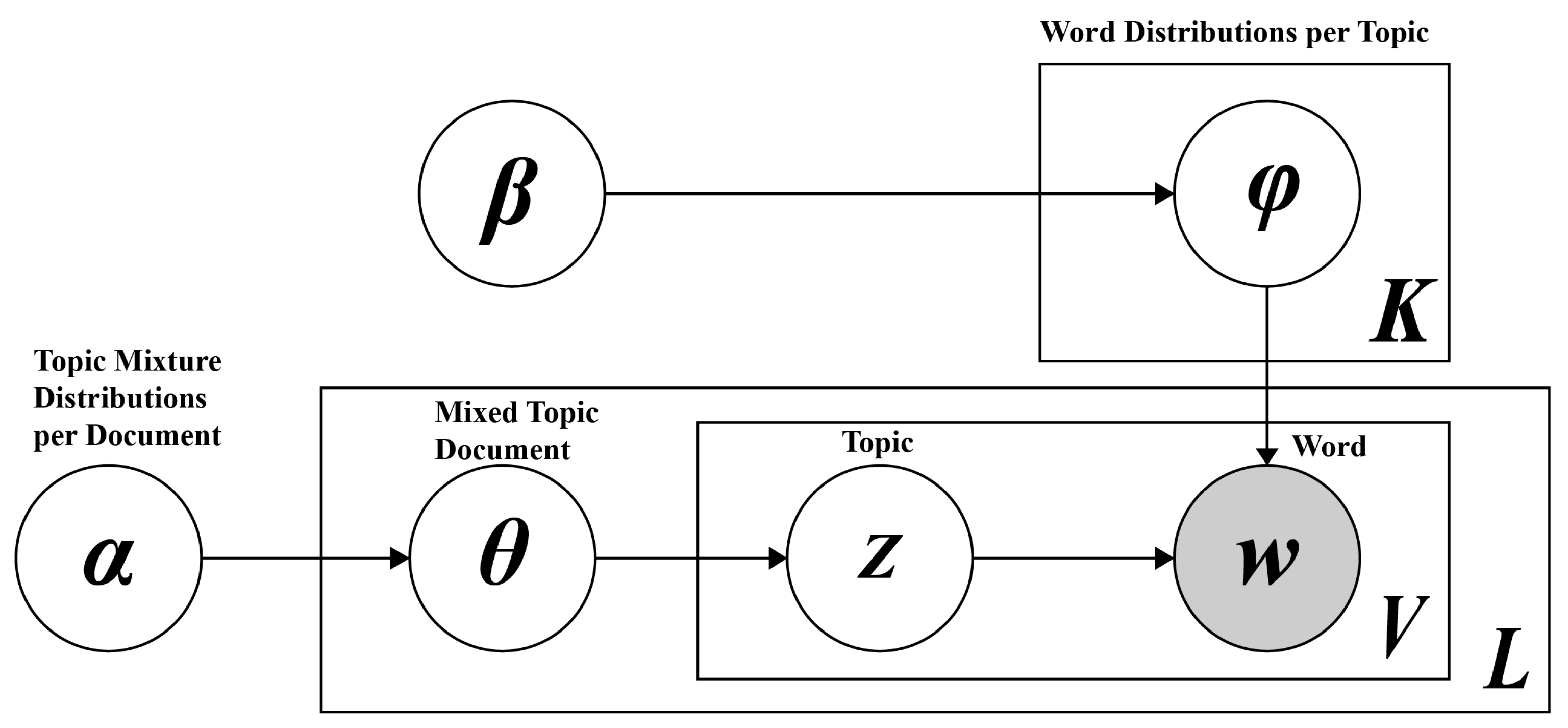
Figure 1. LDA-based topic modeling.
Applsci 15 11937 g001
Figure 2. General framework.
Applsci 15 11937 g002
Figure 3. Some data collection result. Note: “***” indicates anonymized user nicknames to protect personal privacy.
Applsci 15 11937 g003
Figure 4. Topic = 16 Topic model perplexity/consistency score changes with the number of topics.
Applsci 15 11937 g004
Figure 5. Impact of topic number on KL divergence and JS divergence.
Applsci 15 11937 g005
Figure 6. Topic = 4 Topic clustering visualization generated using the pyLDAvis tool, inspired by the Termite visualization principles [41,42]. Source: Created by the authors based on user review texts. The pyLDAvis library is open-source and distributed under the BSD license.
Applsci 15 11937 g006
Figure 7. User preference weight.
Applsci 15 11937 g007
Figure 8. Secondary indicator weight distribution diagram.
Applsci 15 11937 g008
Figure 9. CVAT tool annotation interface.
Applsci 15 11937 g009
Figure 10. Detection results of different algorithms on the scalp detection dataset.
Applsci 15 11937 g010
Figure 11. Algorithm Performance Scatter Analysis.
Applsci 15 11937 g011
Figure 12. Statistical distribution of weight differences across α values.
Applsci 15 11937 g012
Figure 13. Stability of Algorithm Rankings Under Varying α Values.
Applsci 15 11937 g013
Figure 14. Sensitivity analysis results.
Applsci 15 11937 g014
Figure 15. Ranking change curve.
Applsci 15 11937 g015
Table 1. IVNS language evaluation scale for AHP weight calculation.
ImportanceAbbreviationTrue Value Interval TUncertainty Interval IFalse Value Range F
Equally importantEI[0.50, 0.50][0.50, 0.50][0.50, 0.50]
Absolutely less importantAWI[0.50, 0.60][0.35, 0.45][0.40, 0.50]
Extremely less importantEWI[0.55, 0.65][0.30, 0.40][0.35, 0.45]
Less importantMWI[0.60, 0.70][0.25, 0.35][0.30, 0.40]
Generally less importantGWI[0.65, 0.75][0.20, 0.30][0.25, 0.35]
Generally importantGI[0.70, 0.80][0.15, 0.25][0.20, 0.30]
Relatively importantMI[0.75, 0.85][0.10, 0.20][0.15, 0.25]
Generally more importantGSI[0.80, 0.90][0.05, 0.10][0.10, 0.20]
Relatively more importantMSI[0.90, 0.95][0.00, 0.05][0.05, 0.15]
Extremely more importantESI[0.95, 1.0][0.00, 0.00][0.00, 0.10]
Absolutely more importantASI[1.0, 1.0][0.00, 0.00][0.00, 0.00]
Table 2. IVNS language evaluation scale for VIKOR evaluation.
ImportanceAbbreviationTrue Value Interval TUncertainty Interval IFalse Value Range F
Unable to determineUT[0.50, 0.50][0.50, 0.50][0.50, 0.50]
Extremely poorVP[0.50, 0.60][0.35, 0.45][0.40, 0.50]
Very poorVHP[0.55, 0.65][0.30, 0.40][0.35, 0.45]
PoorMP[0.60, 0.70][0.25, 0.35][0.30, 0.40]
Slightly poorSP[0.65, 0.75][0.20, 0.30][0.25, 0.35]
AverageF[0.70, 0.80][0.15, 0.25][0.20, 0.30]
Slightly betterSG[0.75, 0.85][0.10, 0.20][0.15, 0.25]
BetterMG[0.80, 0.90][0.05, 0.10][0.10, 0.20]
Very goodVHG[0.90, 0.95][0.00, 0.05][0.05, 0.15]
ExcellentVG[0.95, 1.0][0.00, 0.00][0.00, 0.10]
PerfectP[1.0, 1.0][0.00, 0.00][0.00, 0.00]
Table 3. Keyword Frequency Statistics.
KeywordTF-IDFFrequency
1Report0.400 1034
2Effect0.399 3945
3Minutes0.381 1953
4Smart0.380 1132
5Precision0.371 945
6Detector0.351 1734
7Hair Loss0.350 10,442
8System0.344 1239
9Equipment0.343 1826
10Professional0.338 2497
11Follicle0.334 11,504
12Detection0.332 8446
13Oil0.305 2256
14Technology0.280 2728
15Scalp0.262 21,312
Table 4. Subject categories and characteristic words.
Theme CategoryTheme Keywords
Topic#1Functional QualityFunction, capability, efficacy, resolution, process, high efficiency, precision,
accuracy, detector, durability, implementation, algorithm, robustness, analyzer, sensitivity, tester, hormone levels, high quality, stability, standardization
Topic#2Product ExperienceRecommendations, Operations, Feedback, Readability, Guidance, User-Friendly, Interface, Evaluation, Impression, Navigation, Aesthetics, Instructional, Exquisite, Service Attitude, Ease of Use, Consultant, Comfort Level, Service Center,
Satisfaction, After-Sales Service
Topic#3Human Factors
Engineering Design
Adjustment, clarity, space, distance, intuitive, height, thickness, convenience,
ergonomics, hand feel, personalization, definition, indications, easy to understand,
design, multi-angle, handy, adjustability, visualization, close-up distance
Topic#4SafetyCleaning, inspection, safety, reminder, standard, caution, verification, sterilization, hidden danger, prudence, prevention, health status, warning, safety hazard,
precautions, sense of security, harmlessness, standard, compliance, stability
Table 5. User requirement indicators for Scalp detector.
Primary
Indicator
Secondary IndicatorRequirement DescriptionThematic KeywordsNumber
A. Functional QualityRecognition AccuracyAbility to detect targets such as hair follicles and dandruffPrecision, identification,
error, resolution, detector
A1
Image ClarityClarity and detail representation of microscope/probe imagingClear, high-definition,
imaging, detail, magnification
A2
Detection SpeedTimeliness of the detection process and efficiency of result outputFast, real-time, response,
process, minutes
A3
Result ConsistencyStability of repeated measurements on the same sampleStable, reliable, repeatability, fluctuation, consistencyA4
B. Product
Experience
Operational EaseSimplified operation workflow and improved interface friendlinessEasy to use, simple, intuitive, friendly, tutorialB1
Contact ComfortComfort of probe-to-scalp contactGentle, imperceptible, soft,
contact, pressure
B2
Learning ResourcesLearning materials to help users quickly master operationTutorial, video, guidance,
instructions, quick start
B3
Result VisualizationIntuitive presentation of detection results and progressPrompt, visualization, report, status, progressB4
C. Human Factors
Engineering
Design
Handle GripErgonomically comfortable
grip design
Grip, fit, anti-slip, fatigue,
handle
C1
Probe AdhesionConformity of the probe to the scalp’s curved surfaceCurvature, conformity,
contact, area, adaptability, angle
C2
Portable StoragePortability of the device and ease of storageLightweight, compact, foldable, storage, volumeC3
Scenario AdaptabilityAbility to adapt to diverse usage
environments
Waterproof, dustproof, thermal drift resistance, drop resistance, shock resistanceC4
D. SafetyMisdiagnosis RiskReliability of identifying high-risk lesionsMisdiagnosis, risk, diagnosis, disease, fungusD1
BiosafetyBiocompatibility and hygiene
assurance of contact components
Non-toxic, low-allergenicity,
biocompatible, sterile, material
D2
Privacy SecuritySecurity protection for user data storage and transmissionEncryption, privacy, storage, transmission, access controlD3
Mishandling ProtectionProtective mechanisms to prevent accidental operationsProtection, locking, warning, insurance, fault toleranceD4
Table 6. Example of Sentiment Polarity and Confidence Analysis for User Comments.
Text ContentEmotional
Polarity
Probability of HeadsConfidence
I used it to detect the status of hair
follicles, and the results seemed quite
accurate, similar to what the doctor said.
Positive (2)0.9520.894
Table 7. Criterion-level pairwise comparison matrix.
ABCD
A[0.50, 0.50], [0.50, 0.50],
[0.50, 0.50]
[0.75, 0.85], [0.10, 0.20], [0.15, 0.25][0.70, 0.80], [0.15, 0.25], [0.20, 0.30][0.25, 0.35], [0.70, 0.80], [0.65, 0.75]
B[0.15, 0.25], [0.80, 0.90],
[0.75, 0.85]
[0.50, 0.50], [0.50, 0.50], [0.50, 0.50][0.55, 0.65], [0.30, 0.40], [0.35, 0.45][0.20, 0.30], [0.75, 0.85], [0.70, 0.80]
C[0.20, 0.30], [0.75, 0.85],
[0.70, 0.80]
[0.35, 0.45], [0.60, 0.70], [0.55, 0.65][0.50, 0.50], [0.50, 0.50], [0.50, 0.50][0.10, 0.20], [0.90, 0.95], [0.80, 0.90]
D[0.65, 0.75], [0.20, 0.30],
[0.25, 0.35]
[0.70, 0.80], [0.15, 0.25], [0.20, 0.30][0.80, 0.90], [0.05, 0.10], [0.10, 0.20][0.50, 0.50], [0.50, 0.50], [0.50, 0.50]
Table 8. Functional quality A pairwise comparison matrix.
A1A2A3A4
A1[0.50, 0.50], [0.50, 0.50],
[0.50, 0.50]
[0.80, 0.90], [0.05, 0.10], [0.10, 0.20][0.75, 0.85], [0.10, 0.20], [0.15, 0.25][0.90, 0.95], [0.00, 0.05], [0.05, 0.15]
A2[0.10, 0.20], [0.90, 0.95],
[0.80, 0.90]
[0.50, 0.50], [0.50, 0.50], [0.50, 0.50][0.90, 0.95], [0.00, 0.05], [0.05, 0.15][0.80, 0.90], [0.05, 0.10], [0.10, 0.20]
A3[0.15, 0.25], [0.80, 0.90],
[0.75, 0.85]
[0.05, 0.15], [0.95, 1.00], [0.90, 0.95][0.50, 0.50], [0.50, 0.50], [0.50,0.50][0.25, 0.35], [0.70, 0.80], [0.65, 0.75]
A4[0.05, 0.15], [0.95, 1.00],
[0.90, 0.95]
[0.10, 0.20], [0.90, 0.95], [0.80, 0.90][0.65, 0.75], [0.20, 0.30], [0.25, 0.35][0.50, 0.50], [0.50, 0.50], [0.50, 0.50]
Table 9. Product Experience B Paired Comparison Matrix.
B1B2B3B4
B1[0.50, 0.50], [0.50, 0.50],
[0.50, 0.50]
[0.90, 0.95], [0.00, 0.05], [0.05, 0.15][0.95, 1.00], [0.00, 0.00], [0.00, 0.10][0.80, 0.90], [0.05, 0.10], [0.10, 0.20]
B2[0.05, 0.15], [0.95, 1.00],
[0.90, 0.95]
[0.50, 0.50], [0.50, 0.50], [0.50, 0.50][0.75, 0.85], [0.10, 0.20], [0.15, 0.25][0.80, 0.90], [0.05, 0.10], [0.10, 0.20]
B3[0.00, 0.10], [1.00, 1.00],
[0.95, 1.00]
[0.15, 0.25], [0.80, 0.90], [0.75, 0.85][0.50, 0.50], [0.50, 0.50], [0.50, 0.50][0.25, 0.35], [0.70, 0.80], [0.65, 0.75]
B4[0.10, 0.20], [0.90, 0.95],
[0.80, 0.90]
[0.10, 0.20], [0.90, 0.95], [0.80, 0.90][0.65, 0.75], [0.20, 0.30], [0.25, 0.35][0.50, 0.50], [0.50, 0.50], [0.50, 0.50]
Table 10. Human Factors Engineering Design C Pairwise Comparison Matrix.
C1C2C3C4
C1[0.50, 0.50], [0.50, 0.50],
[0.50, 0.50]
[0.65, 0.75], [0.20, 0.30], [0.25, 0.35][0.90, 0.95], [0.00, 0.05], [0.05, 0.15][0.75, 0.85], [0.10, 0.20], [0.15, 0.25]
C2[0.25, 0.35], [0.70, 0.80],
[0.65, 0.75]
[0.50, 0.50], [0.50, 0.50], [0.50, 0.50][0.95, 1.00], [0.00, 0.00], [0.00, 0.10][0.70, 0.80], [0.15, 0.25], [0.20, 0.30]
C3[0.05, 0.15], [0.95, 1.00],
[0.90, 0.95]
[0.00, 0.10], [1.00, 1.00], [0.95, 1.00][0.50, 0.50], [0.50, 0.50], [0.50, 0.50][0.25, 0.35], [0.70, 0.80], [0.65,0.75]
C4[0.15, 0.25], [0.80, 0.90],
[0.75, 0.85]
[0.20, 0.30], [0.75, 0.85], [0.70, 0.80][0.65, 0.75], [0.20, 0.30], [0.25, 0.35][0.50, 0.50], [0.50, 0.50], [0.50, 0.50]
Table 11. Security D pairwise comparison matrix.
D1D2D3D4
D1[0.50, 0.50], [0.50, 0.50],
[0.50, 0.50]
[0.70, 0.80], [0.15, 0.25], [0.20, 0.30][0.95, 1.00], [0.00, 0.00], [0.00, 0.10][0.90, 0.95], [0.00, 0.05], [0.05, 0.15]
D2[0.20, 0.30], [0.75, 0.85],
[0.70, 0.80]
[0.50, 0.50], [0.50, 0.50], [0.50, 0.50][0.75, 0.85], [0.10, 0.20], [0.15, 0.25][0.30, 0.40], [0.65, 0.75], [0.60, 0.70]
D3[0.00, 0.10], [1.00, 1.00],
[0.95, 1.00]
[0.15, 0.25], [0.80, 0.90], [0.75, 0.85][0.50, 0.50], [0.50, 0.50], [0.50, 0.50][0.10, 0.20], [0.90, 0.95], [0.80, 0.90]
D4[0.05, 0.15], [0.95, 1.00],
[0.90, 0.95]
[0.60, 0.70], [0.25, 0.35], [0.30, 0.40][0.80, 0.90], [0.05, 0.10], [0.10, 0.20][0.50, 0.50], [0.50, 0.50], [0.50, 0.50]
Table 12. User requirement weights.
Criteria LayerCriteria Layer WeightIndicator LayerIndicator
Layer Weight
IVNS-AHP WeightComposite Subjective WeightConsistency Ratio CR
A0.2907A10.42550.12360.09740.0673
A20.27460.07980.0799
A30.14520.04220.0331
A40.15470.04500.0335
B0.194B10.45240.08780.07270.0625
B20.24960.04840.0677
B30.12210.02370.0566
B40.17590.03410.0531
C0.1557C10.38710.06020.07280.0555
C20.30960.04820.0678
C30.10020.01560.0549
C40.20310.03160.0614
D0.3596D10.42050.15120.07510.0515
D20.24920.08960.0638
D30.09720.03500.0286
D40.23320.08380.0815
Table 13. Evaluation algorithm and training parameters.
ParameterAlgorithm for Evaluation
Faster R-CNNSSD-VGG16YOLOv7YOLOv8n
Representative DirectionHigh-Precision Positioning and Classification [43]Balancing speed and accuracy [44]Best overall
performance [45]
Lightweight and Efficient Design [46]
learning rate1 × 10−31 × 10−31 × 10−31 × 10−3
batch size8888
weight decay5 × 10−45 × 10−45 × 10−45 × 10−4
Momentum0.90.90.90.9
Epochs300300300300
Table 14. Experimental result.
AlgorithmsmAP@50PrecisionRecallF1 ScoreFPSParameters (M)
Faster R-CNN0.710.680.890.77941
SSD-VGG160.870.820.850.833526.8
YOLOv70.830.790.860.824537.18
YOLOv8n0.890.890.870.88553.16
Table 15. Indicator weights under the EWM.
IndicatorMeaningIndicator TypeInformation
Entropy
Weight
mAP@50Core Metric for the Comprehensive Performance of Model Localization and Classification [47]+ 10.78270.1305
PrecisionAssessing the accuracy of model predictions [48]+0.76620.1404
RecallThe ability of a model to detect all positive class samples [49]+0.68940.1865
F1 scoreHarmonic Mean of Precision and Recall [50]+0.74850.1510
FPSKey metrics for evaluating model inference speed and real-time performance [51]+0.77370.1359
Parameters (M)Core metrics for evaluating model size, complexity, and memory consumption [52]20.57380.2559
1 “+” indicates a positive indicator, 2 “−” indicates a negative indicator.
Table 16. Subjective-objective indicator mapping matrix.
User RequirementsmAP@50PrecisionRecallF1 ScoreFPSParameters (M)Algorithm WeightAttribute Classification
A10.350.250.200.20— *1.00Algorithm Core Performance
A2 0.00Hardware Dependency
A3 1.001.00Algorithm Efficiency
A4 0.200.200.300.301.00Algorithm Robustness
B10.00Interaction Design
B2 0.00Industrial Design
B3 0.00Product Operations
B4 0.00Interaction Design
C1 0.00Industrial Design
C2 0.00Industrial Design
C3 0.300.30Hybrid Metrics (Algorithm/Industrial Design)
C4 0.100.100.100.100.40Hybrid Metrics (Algorithm/Hardware)
D1 0.150.400.150.100.80Algorithm Reliability
D2 0.00Materials and Compliance
D3 0.00Information Security
D4 0.00System Design
* Indicators marked as Not Applicable (N/A) are uniformly denoted as “—”. Algorithm weights reflect the correlation between user requirement and algorithm performance.
Table 17. Final weight.
Technical IndicatorsMapping Weight (Wmap)Weights by the EWM (Wtech)Wmap × WtechFinal Weighting (Wfinal)
mAP@500.0582 0.13050.0076 0.1851
Precision0.0672 0.14040.0094 0.2300
Recall0.0469 0.18650.0087 0.2132
F1 Score0.0432 0.15100.0065 0.1590
FPS0.0331 0.13590.0045 0.1097
Params(M)0.0165 0.25590.0042 0.1029
Table 18. Decision matrix.
AlgorithmsmAP@50PrecisionRecallF1 ScoreFPSParameters (M)
Faster R-CNN[0.80, 0.90],
[0.05, 0.10],
[0.10, 0.20]
[0.90, 0.95],
[0.00, 0.05],
[0.05, 0.15]
[0.80, 0.90],
[0.05, 0.10],
[0.10, 0.20]
[0.80, 0.90],
[0.05, 0.10],
[0.10, 0.20]
[0.50, 0.60],
[0.35, 0.45],
[0.40, 0.50]
[0.60, 0.70],
[0.25, 0.35],
[0.30, 0.40]
SSD-VGG16[0.80, 0.90],
[0.05, 0.10],
[0.10, 0.20]
[0.90, 0.95],
[0.00, 0.05],
[0.05, 0.15]
[0.80, 0.90],
[0.05, 0.10],
[0.10, 0.20]
[0.80, 0.90],
[0.05, 0.10],
[0.10, 0.20]
[0.80, 0.90],
[0.05, 0.10],
[0.10, 0.20]
[0.95, 1.00],
[0.00, 0.00],
[0.00, 0.10]
YOLOv7[0.90, 0.95],
[0.00, 0.05],
[0.05, 0.15]
[0.90, 0.95],
[0.00, 0.05],
[0.05, 0.15]
[0.90, 0.95],
[0.00, 0.05],
[0.05, 0.15]
[0.90, 0.95],
[0.00, 0.05],
[0.05, 0.15]
[0.80, 0.90],
[0.05, 0.10],
[0.10, 0.20]
[0.70, 0.80],
[0.15, 0.25],
[0.20, 0.30]
YOLOv8n[0.95, 1.00],
[0.00, 0.00],
[0.00, 0.10]
[0.90, 0.95],
[0.00, 0.05],
[0.05, 0.15]
[0.95, 1.00],
[0.00, 0.00],
[0.00, 0.10]
[0.95, 1.00],
[0.00, 0.00],
[0.00, 0.10]
[0.90, 0.95],
[0.00, 0.05],
[0.05, 0.15]
[0.75, 0.85],
[0.10, 0.20],
[0.15, 0.25]
Table 19. Positive and negative ideal solutions.
IndicatorOptimal SolutionNegative Ideal Solution
mAP@50[0.95, 1.00], [0.00, 0.00], [0.00, 0.10][0.80, 0.90], [0.05, 0.10], [0.10, 0.20]
Precision[0.90, 0.95], [0.00, 0.05], [0.05, 0.15][0.90, 0.95], [0.00, 0.05], [0.05, 0.15]
Recall[0.95, 1.00], [0.00, 0.00], [0.00, 0.10][0.80, 0.90], [0.05, 0.10], [0.10, 0.20]
F1 Score[0.95, 1.00], [0.00, 0.00], [0.00, 0.10][0.80, 0.90], [0.05, 0.10], [0.10, 0.20]
FPS[0.90, 0.95], [0.00, 0.05], [0.05, 0.15][0.50, 0.60], [0.35, 0.45], [0.40, 0.50]
Parameters (M)[0.60, 0.70], [0.25, 0.35], [0.30, 0.40][0.95, 1.00], [0.00, 0.00], [0.00, 0.10]
Table 20. Positive and negative ideal solutions Comprehensive evaluation results of the algorithm.
AlgorithmsImproved IVNS-VIKOR Comprehensive Evaluation Results
Q Value (v = 0.5)S ValueR ValueWk 1ΣP 2Ranking
Faster R-CNN1.00000.54870.109700.00004
SSD-VGG160.70450.50000.106611.00003
YOLOv70.15670.30100.102922.18092
YOLOv8n0.00000.18780.102932.81911
1 Wk denotes the number of pairwise comparisons won. 2 ΣP represents the overall advantage score.
Table 21. Comparison of comprehensive performance with baseline methods.
Method IDMethodological FrameworkEnvironmentWeighting StrategySource
ProposedIVNS-AHP + EWM-VIKORIVNSSubjective: User preferences + AHP (expert); Objective: EWMThis work
M1IVNS-AHP + EWM-VIKORIVNSSubjective: User preferences + AHP (expert); Objective: EWMThis work (Dissolution)
M2IVNS-TODIMIVNSObjective: Similarity measures and information content based on cross-information[53]
M3IVNS-MD-TOPSISIVNSObjective: MD[54]
M4IVIF-AHP-TOPSISIVIFSubjective: AHP[55]
M5IVPFN-AHP-VIKORIVPFNSubjective: PFAHP[56]
M6FIS-AHP-VIKORFISSubjective: FAHP[57]
M7IF-CRITIC-RS-VIKORIFObjective: CRITIC; Subjective: RS[58]
M8TFN-AHP-TOPSIS-VIKORTFNSubjective: AHP[59]
Note: TODIM (an acronym in Portuguese of interactive and multiple attribute decision-making), MD (Maximizing Deviation), IVIF (Interval-Valued Intuitionistic Fuzzy), TOPSIS (Technique for Order Preference by Similarity to Ideal Solution), IVPFNs (interval-valued Pythagorean fuzzy numbers), FIS (fuzzy inference system), IF (Intuitionistic fuzzy), CRITIC (CRiteria Importance Through Intercriteria Correlation), RS (Rank Sum), TFN (triangular fuzzy numbers).
Table 22. Comparison results of different methods.
Method IDSorting Methods1-Faster R-CNN2-SSD-VGG163-YOLOv74-YOLOv8nRanking
Proposed PD - VIKOR   ( Σ P , v = 0.5 ) 0.00001.00002.18092.81914 ≻ 3 ≻ 2 ≻ 1
M1 VIKOR   ( Q , v = 0.5 ) 1.00000.98800.29450.00004 ≻ 3 ≻ 2 ≻ 1
M2 TODIM   ( ϑ ( R i ) )0.00000.61830.78120.84764 ≻ 3 ≻ 2 ≻ 1
M3 IVNS - TOPSIS   ( Γ ^ δ ) 0.21740.64120.76890.92564 ≻ 3 ≻ 2 ≻ 1
M4 IVIF - TOPSIS   ( ϕ j ) 0.30650.72480.82560.88424 ≻ 3 ≻ 2 ≻ 1
M5 FVIKOR   ( Q , v = 0.5 ) 1.00000.69570.14720.00004 ≻ 3 ≻ 2 ≻ 1
M6 FVIKOR   ( Q i , v = 0.5 ) 1.00000.70830.13060.00004 ≻ 3 ≻ 2 ≻ 1
M7 IF - VIKOR   ( e i ) 0.95120.57840.64520.12784 ≻ 2 ≻ 3 ≻ 1
M8 FVIKOR - TOPSIS   ( F C R S i ) 0.12160.63180.78950.96834 ≻ 3 ≻ 2 ≻ 1
Note: ΣP—comprehensive superiority degree (higher is better); Q —VIKOR aggregation index (lower is better); R i —overall dominance degree in TODIM (higher is better); Γ ^ δ —relative closeness coefficient in IVNS-TOPSIS (higher is better); ϕ j —closeness/similarity coefficient in IVIF-TOPSIS (higher is better); Q i —aggregation value in FVIKOR (lower is better); e i —fuzzy distance to the ideal solution (lower is better); F C R S i —comprehensive ranking score in FVIKOR-TOPSIS (higher is better).
Disclaimer/Publisher’s Note: The statements, opinions and data contained in all publications are solely those of the individual author(s) and contributor(s) and not of MDPI and/or the editor(s). MDPI and/or the editor(s) disclaim responsibility for any injury to people or property resulting from any ideas, methods, instructions or products referred to in the content.