Development of an Extreme Machine Learning-Based Computational Application for the Detection of Armillaria in Cherry Trees

Abstract

This paper addresses the automatic detection of Armillaria disease in cherry trees, a high-impact phytosanitary threat to agriculture. As a solution, a computer application is developed based on RGB images of cherry trees and the exploitation of machine learning (ML) models, using the optimal variant among different Extreme Learning Machine (ELM) models. This tool represents a concrete contribution to the use of artificial intelligence in smart agriculture, enabling more efficient and accessible management of cherry tree crops. The overall goal is to evaluate machine learning-based strategies that enable efficient and low-computational-cost detection of the disease, facilitating its implementation on devices with limited resources. The ERICA database is used by following a proper methodology in order to learning and validation stages are completely independent. Preprocessing includes renaming, cropping, scaling, grayscale conversion, vectorization, and normalization. Subsequently, the impact of reducing image resolution is studied, identifying that a size of 63 × 23 pixels maintains a good balance between visual detail and computational efficiency. Six ELM variants are trained: standard, regularized (R-ELM), class-weighted (W1-ELM and W2-ELM), and multilayer (ML2-ELM and ML3-ELM), and classical machine learning approaches are optimized and compared with classical ML approaches. The results indicate that W1-ELM achieves the best performance among tested variants, reaching an accuracy of 0.77 and a geometric mean of 0.45 with a training time in order of seconds.

1. Introduction

In the context of modern agriculture, the incorporation of tools based on artificial intelligence (AI) has acquired increasing relevance to face challenges associated with the early diagnosis of diseases such as Downy Mildew, Alternaria, Cercospora, among others [1]. This project focuses on the development of a computational application for the early detection of the fungal disease Armillaria in cherry trees, using Machine Learning (ML) and Extreme Learning Machine (ELM) models from RGB images. This pathology, difficult to diagnose visually in its early stages, represents a significant threat to fruit production in the Maule Region, the main cherry exporting area in Chile [2].

Agriculture is undergoing a significant transformation with the incorporation of technologies such as AI and the Internet of Things (IoT). These tools enable more efficient crop management through early diagnosis and monitoring systems that optimize resource use, improve traceability, and reduce losses due to disease. This advancement has led to the concept of smart farms, where decision-making is based on automatically processed data and images [3]. Early detection of plant diseases in agriculture helps reduce the spread of infections in crops by preventing early-stage propagation, allowing farmers to treat their crops in time or mitigate the effects on plants [4]. This aspect is also emphasized in [5], which highlights that early detection of crop diseases is crucial as a preventive measure against their spread. However, traditional symptom-based methods often suffer from delays in disease identification. Finally, the study [6] indicates that the early detection of diseases and pests is a key factor for eradicating or minimizing the damage they can cause to agricultural crops. In this context, cherry cultivation is of particular importance for Chile. The country is positioned as the world’s leading exporter, with production expected to reach nearly 657,000 tons by 2024; the majority of its cherry production is destined for China [7]. The reason behind this, it is a symbol of prosperity and good wishes during the Chinese New Year. In this context, demand for Chilean cherries is high, as Chile is one of the few countries in the southern hemisphere where the harvest season coincides with the celebration of this holiday. This international demand imposes high quality standards, so early detection of phytosanitary diseases is essential to ensure the sector’s competitiveness [8].

The state of the art are presented below. Keywords such as Machine Learning, Agriculture, and Extreme Learning Machine were used for the literature review, excluding terms such as Cherry and Armillaria due to the scarcity of specific studies on cherry tree diseases, particularly those caused by the fungus Armillaria. The search, conducted between 2019 and 2025, was carried out in recognized databases such as the Institute of Electrical and Electronics Engineers, Springer, and Science Direct, selected for their focus on research applied to agriculture and engineering. As a result, the 10 most relevant (with more cites) articles were identified, which are presented below.

In [9], the AgroLens system proposes a low-cost smart agricultural architecture for real-time diagnosis of leaf diseases. For this, it uses convolutional neural network (CNN) models such as AlexNet, DenseNet, and SqueezeNet, along with repurposed devices such as servers and on-farm IoT sensors. The results highlight that the SqueezeNet model achieves an accuracy of 97.94% in disease classification. Additionally, the system has the capacity to manage more than 1000 sensors without overloading the network, making it an accessible and efficient solution in rural areas with limited connectivity. In [10], authors introduce kernel ELM (KELM-CYP) to predict crop yield in India based on cropping status, crop type, area, and rainfall. It first merges and normalizes 74,975 historical records. After preprocessing, the model applies a kernel transformation that optimizes the output weights and minimizes the error. KELM-CYP achieves a root mean square error (RMSE) of 0.968, being an architecture that offers greater accuracy and robustness in agricultural approaches. In [11], the integration of Genetic Programming ELM with recurrent neural networks is analyzed to improve plant disease detection and classification. Through preprocessing with adaptive histogram equalization and Kapur threshold segmentation, the model minimizes prediction errors, optimizing image classification using ReLU activations. In [12], farmers struggle to efficiently detect diseases, so the authors apply ELM with the Salp Swarm algorithm (SSA) to optimize the classification of infected leaves. A gray-level co-occurrence matrix (GLCM) and SSA are used to avoid local minima in the optimization of initial weights. This approach achieves an accuracy metric of 97.3% and improves the results by 3% compared to ELM without the algorithm. In [13], an improved YOLOv5 model is used for kiwi flower recognition to optimize pollination. The use of K-Means++ and the attention module in convolutional blocks increases the detection accuracy and improves the efficiency of targeted pollination, with a final accuracy of 96.7% and an mAP of 89.1%. In [14], an IoT-based smart agriculture system is explored, which uses an improved genetic algorithm in combination with ELM to select relevant high-dimensional features. The system identifies Downy Mildew disease on plant leaves through image capture and processing, achieving a 5.71% increase in detection accuracy. In [15], a CNN with a channel attention (CA) mechanism and an ELM classifier are presented. The database employs 50,697 100 × 100 resized images of rice leaves. The model achieves 100% accuracy and area under the curve (AUC) = 1.0, using only 1.97 M parameters compared to over 18 M of DenseNet169. The discussion highlights its efficiency and interpretability that facilitate its deployment in low-resource agricultural devices. In [16], a hybrid model is presented for detecting diseases in tomato leaves. This model combines a CNN with ELM, achieving an accuracy of 97.53%. The method includes image preprocessing and segmentation using K-Means, which improves the accuracy and speed of detection compared to traditional models. In [17], the focus is on detecting leaf diseases using near-infrared (NIR) multispectral images. To do this, it combines ELM with the Grasshopper Optimization algorithm, applying K-Means segmentation and feature extraction. This methodology achieves an accuracy of 97.53%. In [18], an optimized ELM with a binary dragonfly algorithm (BDA) is proposed to automatically classify four foliar diseases (alternaria, anthracnose, bacterial blight, and cercospora) in a microset of 73 images (15 healthy and 58 diseased). After resizing to 256 × 256, converting to Lab, and segmenting with K-Means into three clusters, nine textural features are extracted using GLCM. BDA selects the most informative subset and adjusts weights and biases of the ELM, which reduces the risk of local minima. The classifier achieves 94% accuracy, 92% recall, 95% F-score, and 96% AUC, in one second of training time. In [19], a finite dissimilar compatible histogram leveling (FDCHL) pipeline with a modified ELM (M-ELM) is presented to identify ten leaf diseases from 1000 training and 100 test images. To maximize accuracy at low cost, FDCHL corrects shadows and reduces noise; then K-Means segments the resized diseased region to 512 × 512. Nine GLCM textural features are extracted from the segments, and the most informative subset is retained by fuzzy selection. The classifier achieves a global hit rate (GAR) of 97.87%, a false accept rate (FAR) of 3.20%, and a false reject rate (FRR) of 2.54%, processing each image in 0.10 s. In [20], an L1-norm minimization ELM (L1-ELM) is presented for detecting foliar diseases with low computational cost. L1-ELM selects hidden nodes in a sparse manner and accelerates training. After applying the Kuan filter and extracting color, texture, and shape features, the validated model is trained with 10-fold cross-validation on peach, strawberry, and corn data. L1-ELM achieves an accuracy of 98.5% in peach, 97.7% in strawberry, and 95.7% in corn, with high performance using only 20 active nodes.

In [21], the use of YOLOv5 and the ResNet50 neural network to detect cherry trees affected by Armillaria is explored. In particular, this study has the purpose of noticing on two points of interest: infected leaves and branches, which means stress. For the study, the ERICA dataset is created and the Make Sense platform is used to label images of leaves and branches. Then, deep learning models are applied, obtaining an accuracy of 86.1% with the YOLOv5m variant. It is worth noting that [21] provides a methodology for the detection of Armillaria, being especially relevant since the database is built and made available in this work.

In summary, computational efficiency is a growing field of research in agricultural applications, particularly in areas such as plant leaf disease classification. ELMs are considered ideal for agricultural applications, as Agriculture 4.0 requires real-time processing where not only accuracy but also energy efficiency and implementation simplicity are valued [18]. The article [22] highlights the necessity of continuously retraining computational models, one of the main application domains being the IoT, where large volumes of data are generated and models must be capable of being trained in real time. Moreover, this computational efficiency regarding processing time in agriculture is also emphasized in robotic systems that need to adapt in real time to changing climatic and crop conditions [23]. Even the study by [24], which focuses on improving model training for mobile applications in agriculture, has proposed the retraining of its models. This highlights a growing interest in reducing training time through the use of optimized models, smaller datasets, and improved data processing strategies.

The overall objective of this work was to evaluate different ELM model variants to determine which offers the best performance in the automatic classification of cherry tree health status, prioritizing computational efficiency and field applicability. Our research project aims to address the problem of automatic detection of Armillaria in cherry trees by training different ELM models to identify healthy trees from diseased ones. This automatic detection model will subsequently be integrated into a software application capable of processing cherry tree images and providing a diagnosis. All development will be carried out using MATLAB R2021a software. The main contributions are the following:

• The development of the processed ERICA database, for training simple machine learning models, through processing such as sizing, grayscale conversion, vectorization, normalization, and scaling.
• The introduction of the various models (basic, regularized, unbalanced and multilayer) of the ELM neural network to detect the of Armillaria in Cherry Trees.
• Brute-force optimization of each ELM model, in addition to its exhaustive comparison in terms of performance (accuracy, geometric mean and confusion matrices) and complexity (training time).
• The development of a computational application to suggest whether Armillaria trees are diseased or not using a simple photo taken from any cell phone. This can be considered as a user-friendly software and is destined for farmers due to are the main players in cherry plantations.

This document is organized as follows: Section 2 develops the theoretical framework that supports the key concepts of the project. Section 3 describes the implemented methodology in detail. Section 4 presents the analyses and results obtained. Finally, Section 5 presents the conclusions of the study along with recommendations for future work.

2. Theoretical Framework

One of the main threats to cherry trees is the disease caused by the fungus Armillaria, which affects the tree’s root system, impairing its ability to absorb water and nutrients. Its silent progression, which begins in the roots and culminates in leaf wilting, makes early detection difficult, as shown in Figure 1.

Among the automatic detection approaches for this pathology, there is a Deep learning (DL) model called You only look once (YOLOv), oriented to the detection of objects in images. In the work [21], YOLOv model was used to process images of cherry leaves in order to detect the presence of Armillaria, showing promising results. However, this type of model usually requires large computing power and long training times, which can limit its implementation in contexts with limited computational resources compared to ELM models.

2.1. Armillaria

The genus Armillaria comprises basidiomycete fungi, a group that produces sexual spores in cells called basidia, responsible for one of the most destructive root diseases in woody species, known as root rot (Armillaria root rot). This pathogen affects more than 500 plant species, including fruit trees such as cherry, causing losses due to decreased vigor, production, and premature death of trees. Armillaria is a facultative necrotroph (a pathogen that kills living tissue but can survive on dead matter) capable of destroying cambial tissue (the layer that produces wood and bark) and surviving as a saprotroph (feeding on dead matter). Its life cycle alternates between pathogenic, saprotrophic, and symbiotic phases, and it presents rhizomorphs (cords of melanized hyphae) that grow in the soil and colonize roots from a distance [25]. Rhizomorphs, the main organs of infection, have a protective dark bark and a light-colored pith, with a tip coated with mucilage (a sticky gel) that facilitates adhesion. They grow best between 25 and 28 degrees C, in soils with organic matter, at depths of 2.5 and 20 cm, and can advance up to 1.3 m/yr. Infection combines mechanical pressure, toxins (such as melleolide or armillaria), and cell wall-degrading enzymes (pectinases, cellulases, laccases) that break down components such as pectin, cellulose, and lignin.

In general, Armillaria infection initially manifests as leaf chlorosis, loss of vigor, and early defoliation. Later, cortical necrosis, root rot, and the characteristic presence of white fan-shaped mycelium and melanized rhizomorphs are observed. In advanced stages, physiological collapse of the tree reflects vascular dysfunction and root system degradation. In particular, Armillaria in cherry trees infection begins in the roots, with white mycelium under the bark and dark rhizomorphs. Visible symptoms (leaf yellowing, growth reduction, wilting, and branch dieback) appear late, making detection difficult. The inoculum can persist in the soil for years, and factors such as water stress, high temperatures, or compaction aggravate it. Below, images of cherry trees with/without Armillaria infection are displayed in order to see their visual differences [26].

Climate change increases their risk: higher temperatures and droughts favor rhizomorph growth, and increased ${\mathrm{CO}}_2$ can alter host physiology and its soil microbiota (associated microorganisms). The loss of mycorrhizae (beneficial root-associated fungi) and the increased incidence of secondary pests, such as bark beetles, intensify deterioration [27].

2.2. Image Sizing

ML models require inputs with homogeneous dimensions [28], but the ERICA dataset features snapshots at variable resolutions; therefore, scaling is applied at the start of preprocessing. In MATLAB, imcrop is used, a predefined function in the MATLAB Image Processing Toolbox. This tool allows you to crop an image where the (0,0) coordinate is in the upper left corner [29]. This way, each snapshot is scaled to 1512 × 4032, ensuring that all samples are represented by a fixed-length feature vector. At the same time, with the image sizing, the development of a ML-based computational application for the detection of armillaria in cherry trees could be implemented in any cell-phone, namely without considering hardware/software requirements.

2.3. Grayscale

In digital image processing, RGB images represent each pixel using three channels (red, green, and blue), which requires a larger amount of data to process. Converting to grayscale simplifies this representation to a single channel that describes light intensity levels, where 0 corresponds to absolute black and 255 to pure white. In MATLAB, the conversion is performed following the ITU-R BT.601 recommendation, which weights each channel based on the sensitivity of the human eye to each color, as seen in Equation (1):

$$\mathrm{Gray}=0.299R+0.587G+0.114B$$

(1)

This formula gives greater weight to the green channel because the human eye is most sensitive to light in that wavelength, followed by red and, to a lesser extent, blue. The use of grayscale significantly reduces computational complexity and storage requirements, while preserving essential features such as edges, contours, and textures, sufficient for many classification and pattern detection tasks [30,31].

2.4. Image Resizing

Image resizing is a process by which samples in a set can be increased or decreased in resolution. In this case, the choice is to reduce the size, which allows training times to be shortened without compromising expected performance [32]. Resize is performed by applying interpolation methods, including nearest neighbor, bilinear, and bicubic, each offering different trade-offs between visual quality and computational cost [33]. Lower-order methods, such as nearest neighbor or bilinear, are faster but tend to produce jagged edges or loss of detail. In contrast, bicubic interpolation produces smoother transitions and better preserves edges and textures, which improves the performance of models in classification tasks. In this work, we used bicubic interpolation by cubic convolution, developed by [34], which calculates each new pixel as a weighted combination of the 16 pixels in a $4\times 4$ neighborhood. The weights are calculated using a separable cubic kernel: first, it is cubically interpolated in the x direction using 4 samples per row, and then in the y direction on the 4 intermediate results.

An interpolation function is a special type of approximation function that must exactly match the sampled data at the interpolation nodes. As seen in Equation (2), if f is the sampled function and g is the interpolation function, then

$$g\left(x_k\right)=f\left(x_k\right),\forall x_k\mathrm{node},$$

(2)

for equidistant data, many interpolation functions can be written in the form

$$g\left(x\right)=\sum _k{C}_{k}u\left({\displaystyle \frac{x-x_k}{h}}\right),$$

(3)

where h is the sampling increment, $x_k$ are the interpolation nodes, $u\left(s\right)$ is the interpolation kernel and $C_k$ are coefficients that, in this case, match the original $f\left(x_k\right)$ values due to the properties of the kernel.

The cubic convolution kernel proposed by [34] is symmetric ($u\left(s\right)=u(-s)$), satisfies $u\left(0\right)=1$ and $u\left(n\right)=0$ if n is a non-zero integer, has finite support $(-2,2)$, meaning that each interpolation uses only 4 samples per direction, and is continuous with continuous first-order derivative, avoiding abrupt transitions. According to [34], to maximize accuracy with support-2 cubic polynomials, the kernel should take the form

$$u\left(s\right)=\left\{\begin{array}{cc}{(a+2)\left|s\right|}^3-(a+3){\left|s\right|}^2+1,\hfill & 0\le \left|s\right|<1,\hfill \\ {a\left|s\right|}^3-{5a\left|s\right|}^2+8a\left|s\right|-4a,\hfill & 1\le \left|s\right|<2,\hfill \\ 0,\hfill & \left|s\right|\ge 2,\hfill \end{array}\right.$$

(4)

where a is a shape parameter that controls the sharpness and smoothness of the interpolation. From a Taylor series analysis, he established that to obtain third-order accuracy and a good compromise between smoothness and preservation of detail, the optimal value is $a=-0.5$. This value is widely adopted in practical applications, including MATLAB and OpenCV, because it produces sharper images than the bilinear method without introducing noticeable artifacts.

2.5. Vectorization and Normalization

Vectorization consists of transforming the two-dimensional image matrix, of size $m\times n$, into a one-dimensional vector of length $mn$. This procedure does not alter the intensity values of the pixels, but rather reorganizes their arrangement to obtain a representation compatible with models that operate on feature vectors. In the context of this work, vectorization allows each image to be treated as a single point in a high-dimensional space, facilitating mathematical manipulation and input to machine learning algorithms such as ELM, which require data in vector format [32,35].

Normalization is a procedure that adjusts pixel intensity values to a defined range, with the aim of preventing scale differences from affecting model behavior and improving the numerical stability of learning algorithms. There are different normalization methods, such as standardization (Z-score), mean normalization, or unit norm scaling; however, in this work, Min–Max normalization to the range $[-1,1]$ is exclusively used, since it is the range suggested by the ELM author to ensure the success of its training. In this method, each pixel value x is transformed using the Equation (5):

$$x^{\prime }=2·{\displaystyle \frac{x-x_{min}}{x_{max}-x_{min}}}-1,$$

(5)

where $x_{min}$ and $x_{max}$ correspond to the minimum and maximum intensity values allowed in the image (in 8-bit images, 0 and 255, respectively). This variant was selected following the recommendation of the author of the ELM model [36], since a symmetric range around zero favors numerical stability and improves the convergence capacity, especially when using symmetric activation functions.

2.6. Extreme Learning Machine

ELM is a Single Layer Feedforward Network (SLFN) type neural network in which the weights from the input layer to the hidden layer are randomly assigned and those from the hidden layer to the output are calculated analytically, which allows for very fast training [36]. Figure 2 illustrates the general architecture of the ELM model. This network is composed of an input layer, a hidden layer made up of N neurons, and an output layer. Each input vector $x_j$, corresponds to a previously vectorized image, is connected to all the hidden neurons through a set of weights $w_i$ and biases $b_i$, generating linear combinations that are subsequently transformed by an activation function $g(·)$. The resulting outputs of the hidden neurons make up the matrix H, which represents the output of the hidden layer. This matrix is projected by the output weights ${\beta }_i$, thus obtaining the estimated output of the model $f\left(x_j\right)$. In a simplified way, this output approximates the matrix T, which contains the real labels of the data set.

From this base architecture, different variants arise: the standard ELM, which constitutes the basic model with a single hidden layer and direct calculation of the output weights; the regularized ELM (R-ELM) [37], which incorporates a penalty term ${\parallel \beta \parallel }^2$ on the output weights to avoid overfitting, which only affects the $\beta$ calculation stage without modifying the network structure; the unbalanced ELMs (W1-ELM and W2-ELM) [25,38,39], designed to handle data sets with disproportionate classes through a weighting matrix W applied in the adjustment of the $\beta$ weights, with the aim of compensating for the inequality in the number of samples between classes; and multi-layer ELM (ML-ELM) [40], which extends the original architecture by multiple autoencoder-based hidden layers (AE-ELM) [41], where the output of one layer becomes the input of the next, allowing compressed, sparse, or equal-dimensional representations, with orthogonal weights and biases to improve performance. These variants share the structural simplicity of the original ELM, but adapt its formulation to address problems of regularization, class imbalance [42], or greater representation capacity [38]. Finally, an overall algorithm for all ELM versions is presented below in order to present the learning stage (Algorithm 1):

Algorithm 1: ELM

Input: Data $X\in {\mathbb{R}}^{m\times d}$, labels $T\in {\mathbb{R}}^{m\times k}$; hidden neurons N; activation $g(·)$;                 regularization $C\ge 0$ (optional); sample-weight matrix $W⪰0$ (optional)     Output: Output weights $\beta$; prediction function $f(·)$     1. Initialization. Sample input weights $W_{\mathrm{in}}\in {\mathbb{R}}^{d\times N}$ and biases $b\in {\mathbb{R}}^N$ at random.     2. Hidden layer. Compute $H=g\left(X{W}_{\mathrm{in}}+\mathbf{1}{b}^{\top }\right)$.     3. Compute $\beta$.     •      Standard ELM:$\beta =H^{†}T$.     •      R-ELM (ridge):$\beta ={\left(H^{\top }H+\frac{1}{C}I\right)}^{-1}{H}^{\top }T$.     •      W1/W2-ELM (class-weighted):$\beta ={\left(H^{\top }WH+\frac{1}{C}I\right)}^{-1}{H}^{\top }WT$.     •      ML-ELM: repeat Steps 1–2 for the L hidden layers to obtain $H^{\left(L\right)}$;      then compute $\beta$ on $H^{\left(L\right)}$ as above.     4. Prediction. For a new x: $f\left(x\right)=g\left(x{W}_{\mathrm{in}}+b\right)\beta$; for classification,       $\widehat{y}=argmaxf\left(x\right)$ (or a threshold in binary tasks).

    In other words, the R-ELM is considered for preventing overfitting issue thanks to the balance between empirical and structural risks. Due to the imbalanced dataset, the inclusion of W1-ELM and W2-ELM, which attack imbalanced degree with the a diagonal matrix, come to be mandatory in order to detect not only majority classes but also minority samples. Finally, to explore the paradigm of deep learning (various hidden layers) with the intention of improving accuracy, the ML-ELM based on unsupervised learning thanks to the autoencoder ELMs, with two and three hidden layers are taken into account. All these models are optimized in terms of these hyper-parameters and, then, compared by considering performance and complexity metrics. These results are presented below.

2.7. Metrics

The G-mean represents the geometric mean. In binary classification problems, it considers the accuracy in both classes (healthy and diseased) equally, multiplying the sensitivity (ability to correctly detect the diseased class) and the specificity (ability to correctly detect the healthy class), and then taking the square root of the product. This implies that if a model fails significantly in any class, the value of the G-mean will decrease significantly. The G-mean can be calculated using Equation (6) [43]:

$$\mathrm{G-mean}=\sqrt{{\displaystyle \frac{\mathrm{TP}}{\mathrm{TP}+\mathrm{FN}}}·{\displaystyle \frac{\mathrm{TN}}{\mathrm{TN}+\mathrm{FP}}}},$$

(6)

where TP are the positive elements delivered as positive, TN are the negative elements delivered as negative, FN are the positive elements delivered as negative and FP are the negative elements delivered as positive [43].

On the other hand, accuracy measures how close it is to the desired actual value, and its Equation (7) [26] is given by

$$\mathrm{Accuracy}={\displaystyle \frac{TP+TN}{TP+FP+TN+FN}},$$

(7)

Accuracy is a general metric that measures the relationship between correct and total classifications. It is worth noting that a model will have a better classification capacity if both the mean G and the accuracy are close to 1 [44].

Finally, the training time (TT) will be used as a key metric to estimate the computational efficiency of each variant. To do this, the cputime function of the MATLAB [45] environment will be used. This function measures the total central processing unit (CPU) time consumed from the start of the script execution until its completion, in order to determine the configuration of the number of hidden neurons. This measure offers a direct approximation to the computational complexity of the model, since it reflects the time cost required to adjust the internal parameters based on the input and output data [46].

3. Methodology

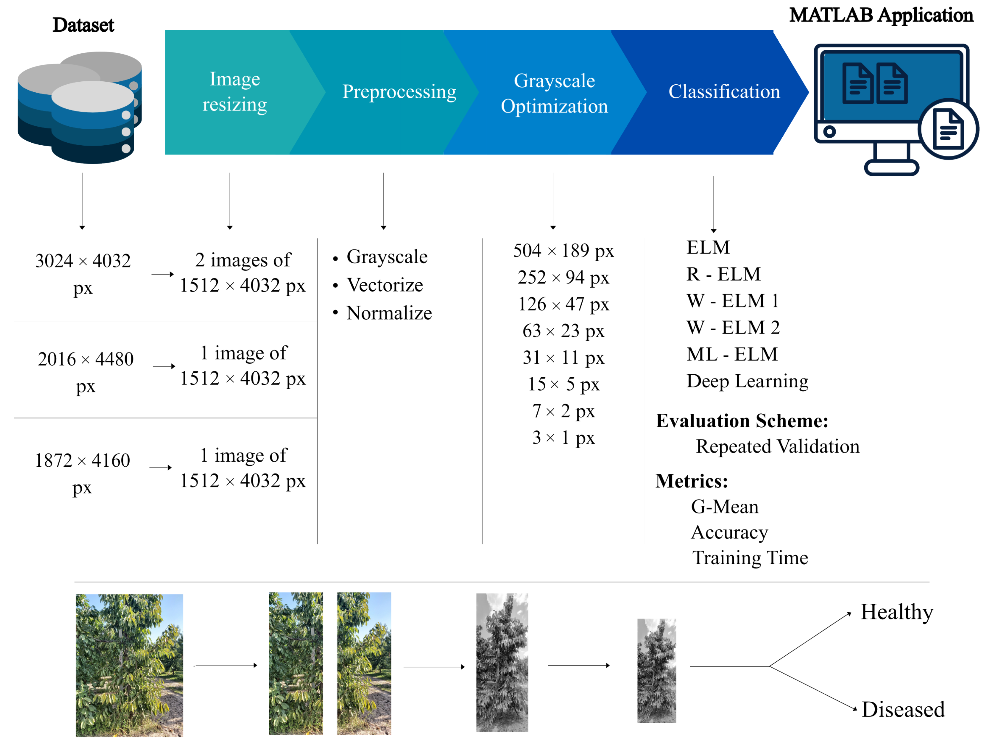
The methodology followed consists of five main stages: (i) selection and organization of the ERICA dataset, (ii) sizing and preprocessing of the images, (iii) scale optimization, (iv) training of different ELM variants, and (v) performance validation using classification metrics. Figure 3 summarizes this workflow, which is detailed in the following subsections.

3.1. Dataset

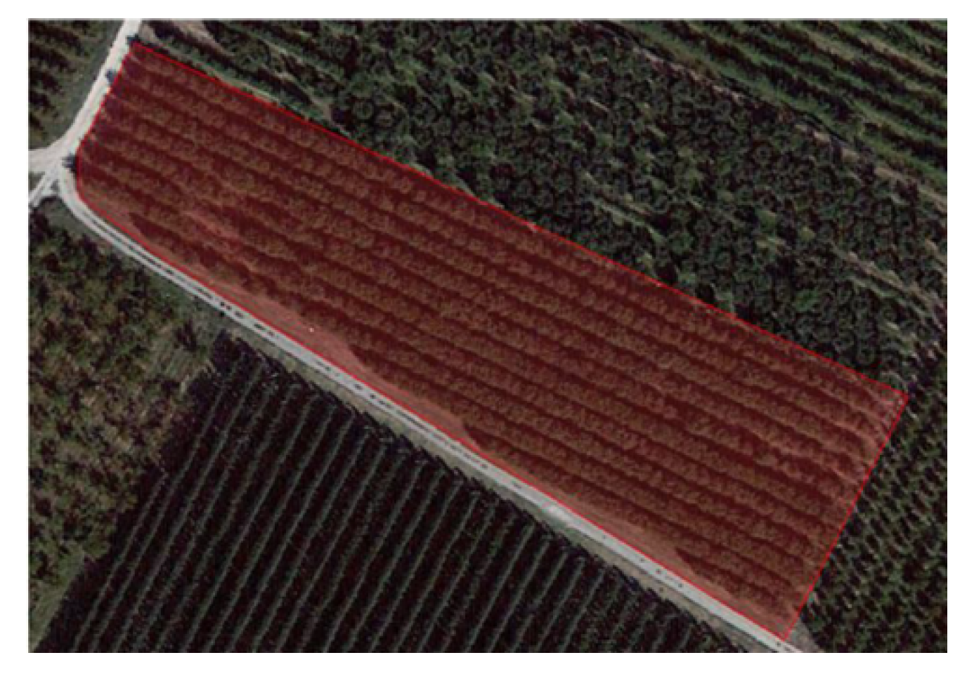
According to Figure 3, the dataset called ERICA, referenced in the article [21], where its samples are located in Western Macedonia, Greece, with a latitude of $40.81008$ and longitude $21.8006$, using the World Geodetic System (WGS) format, as seen in Figure 4. It was an agricultural environment that benefits from advanced technologies for the detection and characterization of diseases in sweet cherry trees [47].

The choice was made to use images in RGB format, as they allow for a more intuitive interpretation and adaptation for both the programmer and the farmer, who is the end user of the application (see Section 4.3). Furthermore, this format would facilitate practical implementation, since the photographs can be captured with conventional devices, such as mobile phones and/or digital cameras. The images are subsequently transformed to grayscale for processing, maintaining their original resolution and reducing computational complexity by a factor of 3. In future work, it is considered appropriate to explore the use of RGB images without transforming them to grayscale or considering multispectral photos, in order to improve the diagnostic accuracy of the system through ELM in the hypercomplex domain [36].

As shown in Figure 4, the study area containing the dataset can be seen. It should be noted that this image was captured by an unmanned aerial vehicle (UAV). The database has 5807 images, including UAV images of the terrain, multispectral images, and RGB images of cherry trees, which are separated into images of healthy and diseased trees, with different degrees of disease affectation.

Below is

Table 1. Summary of images classified by year, date, tree status, resolution, and quantity.

Year	Date	State of the Tree	Dimension	Amount
2021	3 November 2021	Armillaria	3024 × 4032	29
		Healthy	3024 × 4032	548
	8 July 2021	Armillaria	1872 × 4160	22
		Healthy	1872 × 4160	555
	16 September 2021	Armillaria	3024 × 4032	29
		Healthy	3024 × 4032	548
2022	13 July 2022	Armillaria	1872 × 4160	59
			2016 × 4480	4
		Healthy	1872 × 4160	479
			2016 × 4480	35
	26 May 2022	Armillaria	3024 × 4032	64
		Healthy	3024 × 4032	510
Total				2882

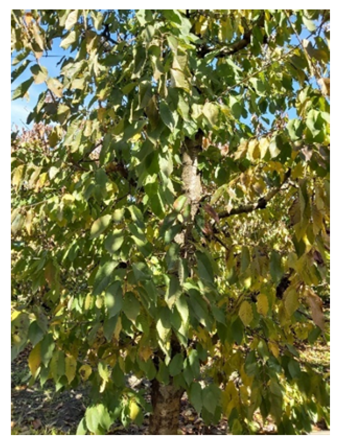
which presents a summary of the number of images used in the dataset. These are separated into two years: 2021 and 2022. In 2021, three dates are recorded and in 2022, two dates, divided into different image resolutions: 3024 × 4032, 1872 × 4160 and 2016 × 4032 [47]. As mentioned, a database called ERICA [47] was selected, which comes from the [21] study, and which contains images of cherry trees in different health states. The images are in RGB format, as in Figure 5.

For the simplicity of this study, only RGB images of healthy and diseased trees are studied. The dataset is split by year because the images used for training and testing should not match, to avoid overfitting. Images from 2021 are selected for the training stage, as this set contains a larger number of samples, allowing for more robust learning. In contrast, images from 2022 are used for the testing stage, as a large amount of data is not required at this stage. This also allows the neural network to be validated using previously unobserved data, namely a realistic situation. Images from 2021 are used for training, corresponding to a total of 1724 images (1651 healthy and 73 diseased), while the remaining images are used for testing, totaling 1151 (1024 healthy and 127 diseased). As can be seen, the imbalance degree of the dataset is $73/1651=0.0442$ and $127/1024=0.1240$ for learning and validation stages, respectively. Namely, in both phases, the imbalance ratio is severally notorious since a balance dataset is distinguished by a relation of 1 and some imbalanced datasets are relationships of 0.3. Due to these imbalance degrees, G-mean metric should be considered more than the accuracy metric in order to majority and minority samples can be identified, and, therefore prevention, detection, evaluation and treatment of armillaria in cherry trees.

To combat with this issue (data with imbalanced class distribution), the unbalanced ELMs (W1-ELM and W2-ELM) are particularly used in this work, which are able to standardize to balanced data. As future direction lines, a complementary alternative to the use of weighted algorithms is to apply training set restructuring techniques, such as minority class oversampling. In particular, the Synthetic Minority Oversampling Technique (SMOTE) is recommended, widely recognized for its effectiveness in unbalanced classification problems. SMOTE technique can be summarized by the following steps: identify the Imbalance, focus on the minority, create synthetic samples, and increase minority.

It is important to note that the original study [21] used training and test samples from both years (2021–2022), an approach that can be considered biased and inaccurate. This methodology is not followed in our work, since mixing periods would not allow the model’s generalization to be adequately evaluated, making it impossible to predict armillaria disease in an upcoming season. Therefore, images from 2021 were used for training and 2022 for testing, in order to avoid overfitting and simulate a realistic scenario. Namely, we split the data by years in order to verify the model’s adaptability to unseen data, namely it a smart way to prevent data leakage. However, it is recognized that there may be year-related distribution differences in tree images (photography season, lighting conditions, stages of the tree growth cycle, imaging equipment parameters, among others, situations that are almost impossible to control in practice). These differences can affect the model’s generalization performance, and it can be considered a realistic scenario, which would occur in an upcoming management due to factors beyond our control. In this sense, we attempt to evaluate the system performance following the proposed methodology, a year by training phase and another year for testing samples.

Notice that in Chile, the presence of Armillaria has been reported primarily in southern areas of the country, where it affects various forest species. Although isolated cases have been reported in areas near the Maule Region and in parts of the central zone, there is no formal evidence indicating that Armillaria is a disease that directly impacts cherry trees in this region [37]. To the best of our knowledge, there is not a dataset of Armillaria in cherry trees in Chile. In this sense, we adopt as inputs for our study the ERICA dataset from Greece since since it is available for free as as previously shown.

3.2. Image Sizing

The ERICA database contains images captured at different resolutions, which poses a challenge for training ML models, as these require dimensionally homogeneous inputs. In total, three predominant resolution formats are identified: 3024 × 4032, 1872 × 4160, and 2016 × 4480 pixels. To unify the dimensions of all images, the standard resolution is set at 1512 × 4032 pixels. Based on this decision, the following cropping is applied:

• The 3024 × 4032 images are divided into two equal parts on the horizontal axis (X axis), generating two images of 1512 × 4032 pixels each.
• 1872 × 4160 images are cropped 360 pixels from the right edge (X axis) and 128 pixels from the bottom edge (Y axis), resulting in 1512 × 4032 pixel images.
• 2016 × 4480 images are cropped 504 pixels from the right edge (X axis) and 448 pixels from the bottom edge (Y axis), you also get 1512 × 4032 pixel images.

This procedure generates a new dataset with images of uniform size, which facilitates subsequent processing and ensures compatibility with the models used. The dataset consists of 4281 healthy individuals and 324 diseased individuals, for a total of 4605, with a ratio of 13.2:1.

Table 2. Summary of images classified by year, date, tree status, and quantity, after the trimming process.

Year	Date	State of the Tree	Amount
2021	3 November 2021	Armillaria	58
		Healthy	1096
	8 July 2021	Armillaria	22
		Healthy	555
	16 September 2021	Armillaria	58
		Healthy	1096
2022	13 July 2022	Armillaria	63
		Healthy	514
	26 May 2022	Armillaria	123
		Healthy	1020
Total			4605

below presents a summary of the images classified by year, date, tree condition, and quantity:

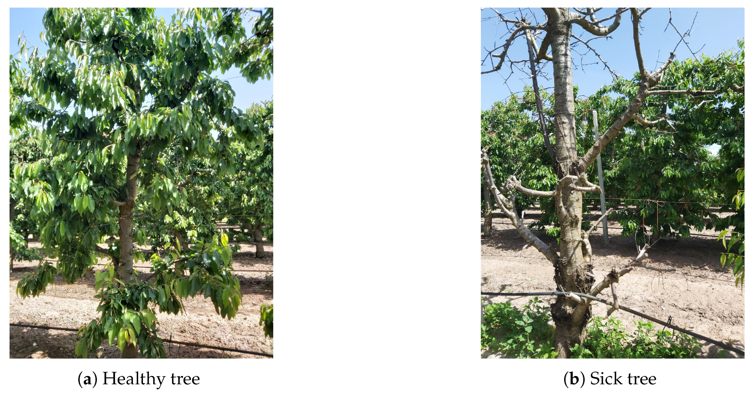
As mentioned, the entire study takes the entire tree as the research object. This happens due to it is unfeasible to obtain an accurate dataset from a macroscopic perspective for detection. In this sense, in Figure 6a,b, illustrative examples of a healthy tree and a sick tree are shown, presented as a random sample for both classes. These can be considered as the input of the ELM models after the digital image processing presented below.

3.3. Preprocessing

Image preprocessing encompasses a series of techniques that allow for the efficient construction of a training database for ML. In general, it constitutes an essential step in machine learning systems applied to classification tasks, as it directly determines the quality, consistency, and relevance of the data entering the model. Indeed, learning accuracy depends largely on the samples used presenting homogeneous and representative characteristics of the phenomenon under study. Various preprocessing techniques are implemented to guide the study. This is because the original images are in RGB format and have a resolution of 1512 × 4032, which makes processing more complex and requires considerable time for the code to complete. Among the techniques used in this work are grayscale conversion, normalization, scaling, and vectorization. Proper preprocessing not only reduces computational complexity but also improves the model’s generalization capabilities by providing more consistent and representative inputs [48].

First, the images are renamed by assigning numbers, since images with the same name exist on different dates. This allows the images to be grouped into folders organized by category: healthy trees from 2021, diseased trees from 2021, and the same for images from 2022, thus avoiding data loss.

Preprocessing begins with code that accesses these folders to independently process the images of healthy and diseased trees. The images are scaled to different resolutions. They are subsequently converted to grayscale to simplify analysis and finally, vectorized into one-dimensional matrices for easier handling in subsequent processing stages.

Once vectorized, the images of healthy and diseased trees were randomly shuffled to prevent clumping and then normalized on a scale of −1 to 1 to ensure compatibility of the trained models, improving the accuracy of the variants. Finally, the preprocessed images are stored for easy use in subsequent analyses. Additionally, an .xlsx file was created where the labels corresponding to each image were stored, indicating whether it represented a healthy tree (0) or a diseased tree (1), thus ensuring proper data tracking. In order to allow to reproduce, expand or improve the results, the processed data set can be found in: https://drive.google.com/file/d/19If-DiwdfxIK2HGCsGnHIN_4r8CJekaM/view?usp=sharing (accessed on 8 August 2025).

3.4. Image Scaling Optimization

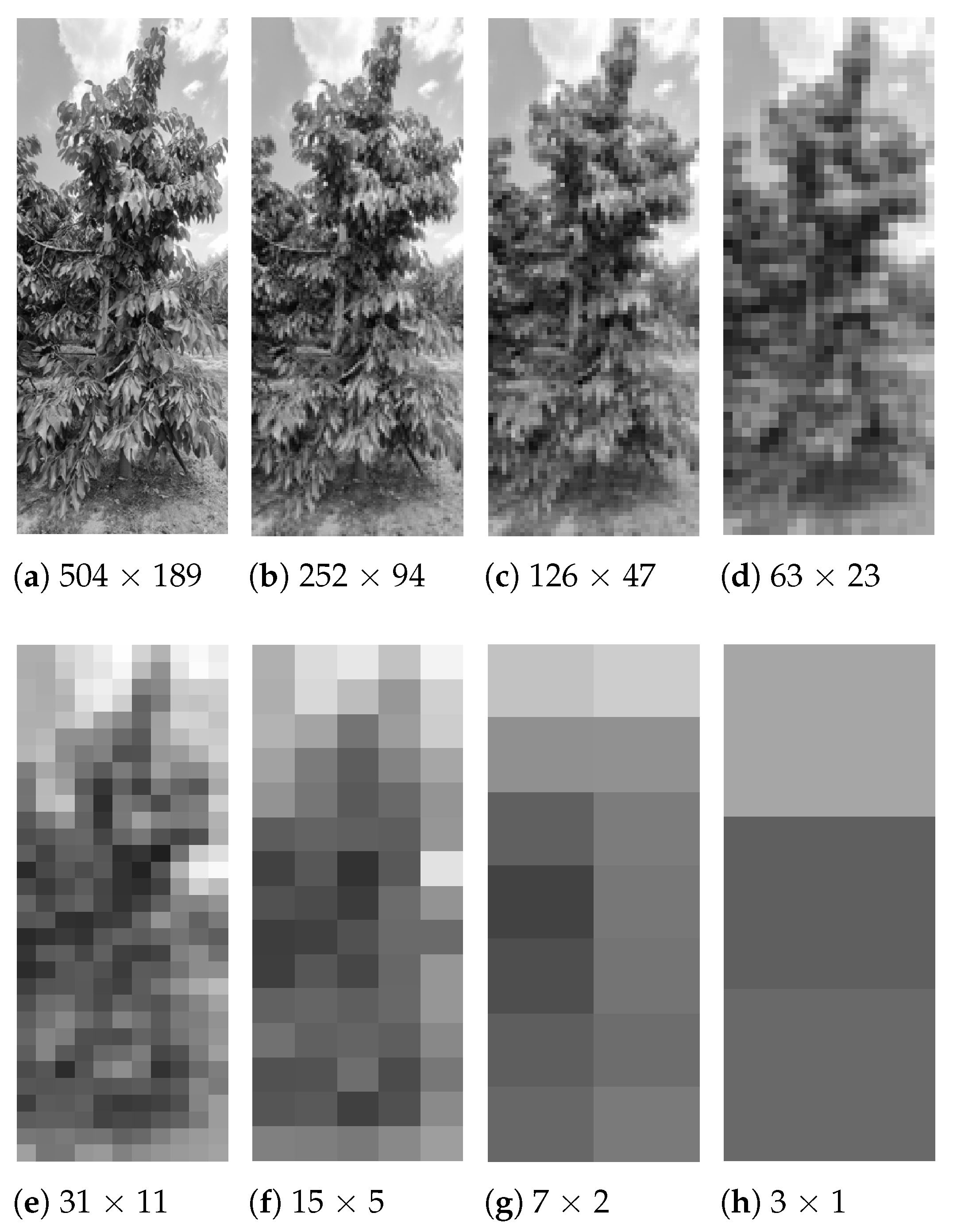
In order to evaluate the impact of visual information reduction on model performance, an image optimization process is implemented. The original image, with a standard resolution of 1512 × 4032 pixels, is successively divided along both the horizontal (X) and vertical (Y) axes, applying divisions in powers of two, i.e., $2^n$. This procedure allows observing the model’s behavior under different levels of spatial compression. Figure 7 shows examples of the visual change of an image as its dimension is reduced.

Eight divisions are considered from $2^3$ to $2^{10}$, generating blocks of decreasing size that are from 504 × 189 to 3 × 1. It is decided to start the process from $2^3$, since lower resolutions do not allow the code to run on a local computer due to memory and processing limitations. Each of the generated subsets is used to train the standard ELM model, since this variant presents the simplest architecture among those proposed, which translates into a shorter training time. In addition, it allows establishing a performance baseline to apply to more complex variants, such as R-ELM, W-ELM, or ML-ELM.

Subsequently, the accuracy and geometric mean metrics are evaluated in both the training and testing sets, in order to analyze the relationship between the size of the processed image and the classification capacity of the model.

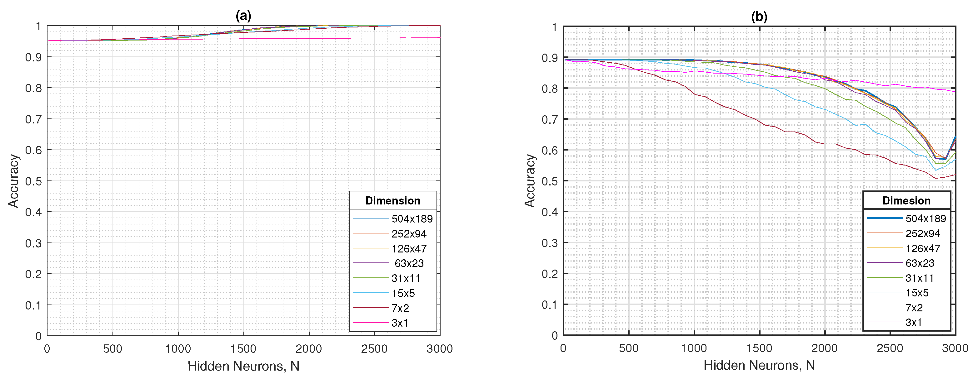
In Figure 8a,b, the accuracy in terms of the hidden neurons for training and testing phases are shown, respectively. For learning set, the performance does not show significant changes at any of the resolutions evaluated. Instead, for validation set, the accuracy is near to 0.9 in the first hidden neurons. The dimension of figure acquires importance when the number of hidden nodes increase, by showing an special detriment for 31 × 11 or below resolution images.

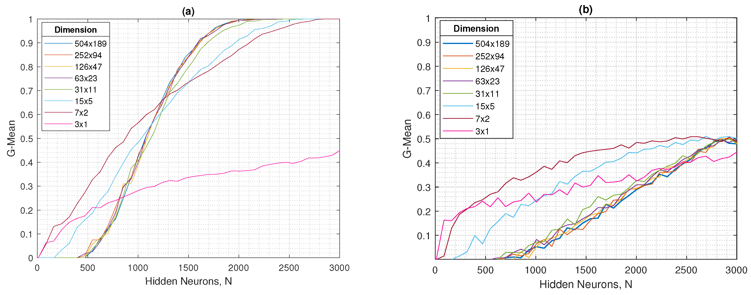
In Figure 9a,b, the geometric mean, both in training and testing, presents initial values close to zero in practically all resolutions. However, starting at approximately 500 hidden neurons, these values begin to increase progressively, reaching a maximum of 1 in training and 0.5 in testing.

In general terms, the different resolutions evaluated show consistent behavior: in the training set, except for the tests with 3 × 1 resolution, both the accuracy and the mean G tend to increase steadily to values close to 1, while in the test set both metrics present greater variability, reflecting an incipient overfitting as the number of hidden neurons increases. This pattern remains stable from 504 × 189 to 63 × 23 pixels, resolutions in which the classifier maintains an acceptable balance between accuracy ($\approx 0.9$ in testing) and mean G ($\approx 0.5$ in testing), even with a drastic reduction in the input size. However, starting from 31 × 11 pixels, the performance degradation becomes evident, which coincides with the visual loss of distinctive features in the images and limits the model’s ability to discriminate between classes. Consequently, the 63 × 23 resolution can be considered an optimal balance point, being the last dimension that maintains performance stability and, at the same time, offers a reduced computational cost compared to higher resolutions, a key aspect for applications in resource-limited scenarios.

3.5. Implementation of ELM Variants

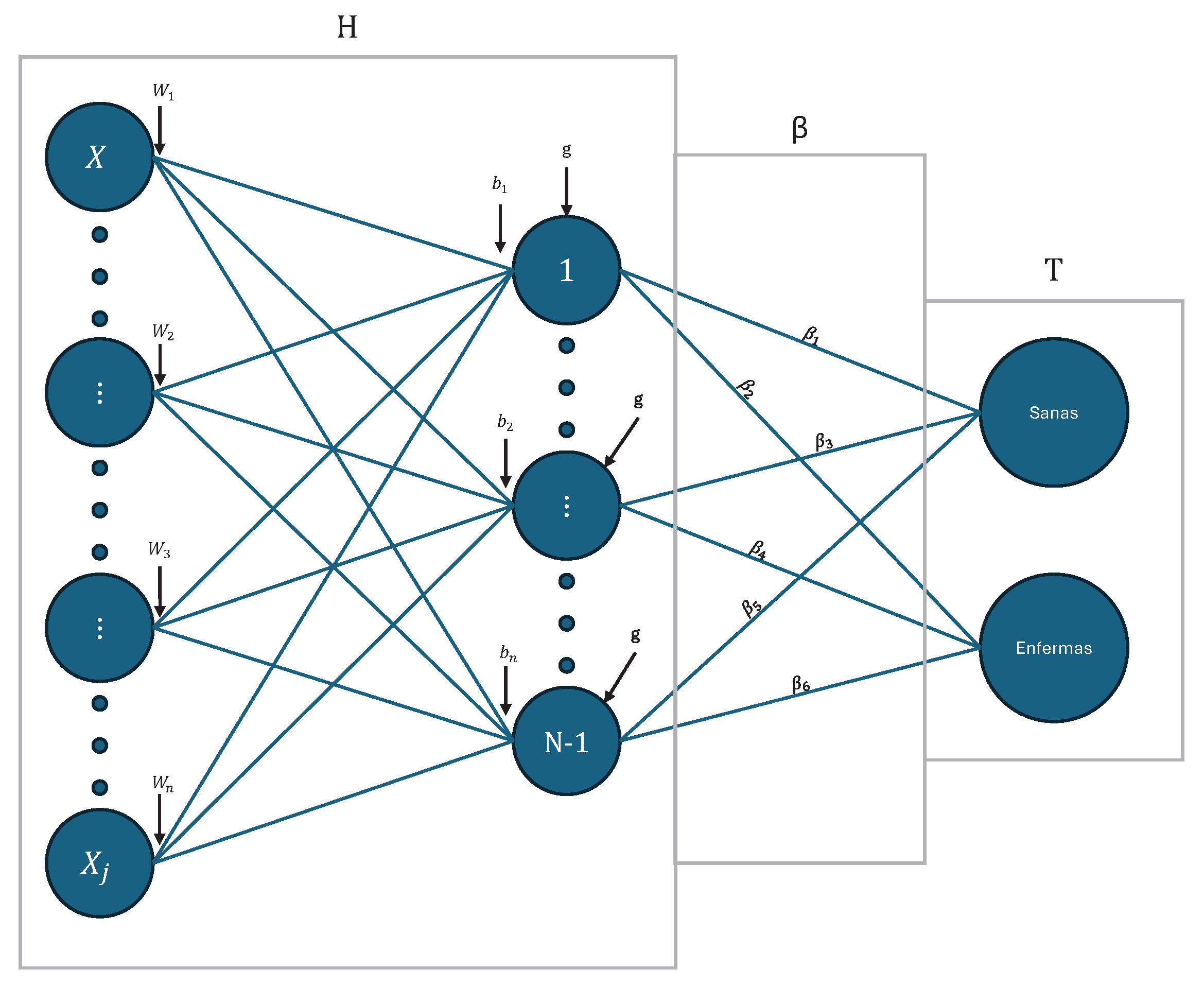
In this stage of the work, six variants of the ELM model are implemented, with the aim of comparing their performance in classifying images of healthy and diseased cherry trees. The variants used are: ELM, R-ELM, W1-ELM, W2-ELM, ML2-ELM, and ML3-ELM. Each of these models is trained using the set of preprocessed images with a unified resolution of 63 × 23 pixels. For all variants, the sigmoid activation function is used, and the input weights are initialized randomly, as is characteristic of the ELM network. In the weighted variants (W1 and W2), weight matrices are incorporated that assign greater relevance to the samples of the minority class. In the case of the multilayer ELM, two and three hierarchically connected hidden layers are used, where each layer applies orthogonal projections to improve data representation.

To ensure a reliable evaluation, each variant was trained ten times following a Monte-Carlo approach, by using a fixed random seed for reproducibility, debugging, stable comparisons, shared results, and experiment control. This involved repeating the training with different random initializations (and data partitions when relevant) to reduce the influence of chance factors. By averaging the results of these runs, representative performance measures were obtained, providing a more robust view of the expected behavior of each variant compared to single-run results. As mentioned in dataset section, images from 2021 were used for training and 2022 for testing, in order to avoid overfitting and simulate a realistic scenario, namely for predicting healthy/sick cherry trees in a future year.

3.6. Hyperparameters

Effective implementation of the different ELM models requires meticulous tuning of their hyperparameters, which is crucial to obtaining optimal results. The procedure is performed by brute force in this work, by exploiting the ELM approaches that do not require iterative processes in the learning stage. The first hyperparameter is the regularization parameter (C), used for R-ELM and W-ELM, and is represented as a vector $C=\left[2^n\right]$, which spans values for n from $-20$ to 20 in regular intervals of four units. This adoption is very common in the ELM context. The second hyperparameter is the number of hidden neurons N, which is used in all variants. This is defined as a 40-element vector ranging from 10 to 3000 hidden neurons. In the specific case of the ML-ELM with three hidden layers, this vector contains 20 values, with the aim of optimizing training times. It is worth noting that a number of hidden neurons equivalent to 80% of the total samples is not used, since this configuration does not present stable behavior in the performance graphs. The third hyperparameter, which remains constant across all tested variants, is the activation function. The sigmoid function is used, widely adopted in machine learning models for its simplicity and effectiveness [49].

Although hyperparameter optimization was performed by exhaustive search prioritizing the G-Mean metric, complementary hyperparameter combinations that involved a smaller number of hidden neurons were selected, in order to improve computational efficiency and reduce model complexity. The choice of the fine-grid approach was intended to simplify the tuning process, taking advantage of the computational resources available for this study, a high-power server. However, we recognize that there are more efficient alternatives, such as Bayesian optimization [50] or methods based on swarm intelligence [51,52,53], which allow considerably reduced search times. In fact, in recent research, we have used algorithms such as Artificial Bee Colony and Aquila Optimizer for tuning ELM and R-ELM networks [51,52], achieving in each test approximately 99% of the performance obtained with an exhaustive search, but using only approximately 5% to 16% of the total time depending on the method, network and application, outperforming random search in the process with a slight increase in computing time. Therefore, although exhaustive search was adequate for the objectives of this work, adaptive soft computing techniques with a heuristic optimization approach are planned to be incorporated in future studies to improve efficiency, especially in agricultural applications, where computing capacity may be low or faster response times are required.

3.7. Metrics

The performance metrics used are accuracy, geometric mean, and training time, to comprehensively compare performance and complexity. For each model, the accuracy and geometric mean are calculated and plotted in terms of their hyperparameters: number of neurons for all ELMs and regularization parameters for R-ELM, W1-ELM, and W2-ELM. Training time is recorded for each run to compare the computational efficiency of each method. Furthermore, the standard deviation of each metric is calculated to assess the stability of the results obtained.

3.8. Software and Hardware

For this study, MATLAB R2024a software is used. To measure this time, the cputime command is used in MATLAB R2021a software. The hardware used corresponds to an Intel Core i5-11400H processor, with a 2.70 GHz CPU (6 cores), 6 GB of RAM, and an NVIDIA GeForce GTX 1650 graphics card. Note that these characteristics govern the results in terms of training time (computational complexity) as well as prediction speed. These results are presented and discussed for ELM models and for other ML approaches in

Table 3. Comparison of the models in terms of hidden neurons, regularization parameter, accuracy, G-mean, and training time.

Model	N	C	Accuracy	G-mean	TT (s)
ELM	2847	Not applicable	0.86 ± 0.0206	0.30 ± 0.0350	44.0516 ± 2.1143
R-ELM	2770	$2^{12}$	0.63 ± 0.0185	0.47 ± 0.0245	2.0766 ± 0.2869
W1-ELM	2770	$2^{12}$	0.77 ± 0.0048	0.45 ± 0.0156	6.2406 ± 0.4564
W2-ELM	1083	$2^8$	0.78 ± 0.0094	0.44 ± 0.0269	8.1859 ± 0.1516
ML2-ELM	N1 = 2540	Not applicable	0.73 ± 0.0371	0.43 ± 0.0413	8.1859 ± 0.0205
	N2 = 2233
ML3-ELM	N1 = 2528	Not applicable	0.721 ± 0.0159	0.43 ± 0.0232	18.6536 ± 1.6570
	N2 = 797
	N3 = 2528

and

Table 4. Comparison of the models in terms of accuracy, G-mean, training time, and prediction speed.

Model	Accuracy	G-mean	TT (s)	PS (obs/s)
Cosine KNN	0.9285	0.617	57.442	927.867
Medium KNN	0.9225	0.459	24.416	1614.200
Cubic KNN	0.9203	0.400	293.154	74.195
Weighted KNN	0.9194	0.380	304.142	1582.430
Fine KNN	0.8243	0.311	13.647	1613.880
Linear Discriminant	0.8410	0.255	18.883	3951.740
Wide Neural Network	0.9047	0.430	32.193	7413.000
Trilayered Neural Network	0.8961	0.375	210.684	7486.310
Medium Neural Network	0.8948	0.387	30.456	7118.230
Narrow Neural Network	0.8928	0.417	33.302	7577.900
Bilayered Neural Network	0.8921	0.411	117.727	7741.210
Kernel Naive Bayes	0.7961	0.390	858.002	20.773
Gaussian Naive Bayes	0.7355	0.378	10.798	3200.040
Quadratic SVM	0.9285	0.480	46.583	3576.560
Cubic SVM	0.9278	0.618	74.560	3162.630
Efficient Linear SVM	0.9278	0.440	11.127	7044.350
Coarse Tree	0.9273	0.290	14.854	7318.230
Medium Tree	0.9172	0.340	12.329	7495.720
Fine Tree	0.8670	0.303	8.525	7576.05
Multilayer Perceptron	0.9303	0.221	48.0	7285.453
W1-ELM	0.7700	0.450	6.240	9834.960

, respectively.

4. Results and Discussion

4.1. Hyperparameter Optimization

To display the hyperoptimization results of the ELM-based models, a line graph was used for the standard ELM, contour plots for the R-ELM W1-ELM, W2-ELM, and ML2-ELM variants, and a point cloud for the ML3-ELM approach. It is done for both metrics, the accuracy and G-mean. In selecting the best hyperparameters for each model, G-mean was prioritized for its ability to balance sensitivity and specificity in highly unbalanced scenarios, unlike accuracy, which reflects only the overall hit rate. In the following of the paper, outcomes are presented the testing stage since in this comparison with the state of the art can be properly done, namely in the same conditions (without the knowledge of artificial intelligence-based models in the test samples).

4.1.1. Standard ELM

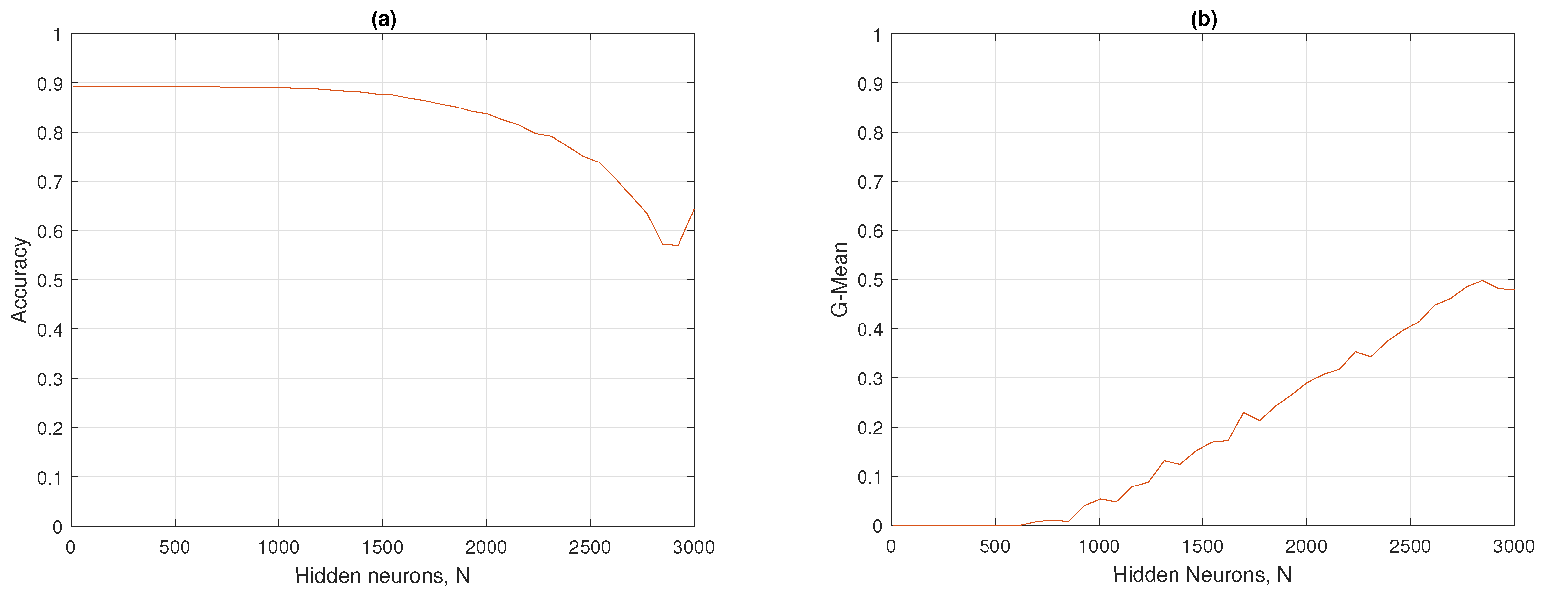
In Figure 10a,b, the accuracy and G-mean of the standard ELM on hidden neurons are shown. The accuracy on the test set peaked from $N=10$ to $N\approx 1000$, with a value of approximately 0.89, and then decreased dramatically. On the other hand, in Figure 10b, the G-mean started with values from 0 to $N\approx 700$, and then reached its maximum at $N\approx 2847$, with a mean G of 0.49. The optimal hyperparameter for the standard ELM was found at $N\approx 2847$, presenting an accuracy of 0.86 and a mean G of 0.49.

4.1.2. Regularized ELM

The contour plots of the accuracy and mean G are shown in Figure 11a,b. In Figure 11a, the ELM-R model achieved an accuracy of approximately 0.88 across all hidden neurons. The performance in this metric tends to be negative for high hidden neurons (>2500) and regularization parameters greater than 1 ($2^0$).On the other hand, in Figure 11b, the G-mean reached values of 0 in all hidden neurons, except for the $N\approx 2993$ with a $C\approx 2^4$, obtaining a mean G of 0.48. To find an optimal value between these results, it was decided that in the $N\approx 2770$, with a regularization hyperparameter of $C\approx 2^{12}$. Note that in this configuration ($N=2993$ and $C=2^4$), the R-ELM maximized its performance with a G-mean of 0.48 and an accuracy of 0.63.

4.1.3. Unbalanced 1 ELM

In Figure 12a,b the contour plots of the accuracy and G-mean of the W1-ELM are observed. In Figure 12a, it was observed that the accuracy started to reach optimal values starting at $N\approx 1237$ with a $C\approx 2^{12}$. On the other hand, in Figure 12b, the G-mean started to reach optimal values at $N\approx 87$ with a $C\approx 2^0$. The hyperparameters that maximized the performance of the W1-ELM were $N\approx 2770$ with a $C\approx 2^{12}$, achieving accuracy values of approximately 0.77 and a geometric mean close to 0.45.

4.1.4. Unbalanced 2 ELM

Figure 13a,b show the contour plots of the accuracy and G-mean of the W2-ELM. In the graph in Figure 13a, it was observed that optimal values began to be obtained from $N\approx 1543$ with a $C\approx 2^4$. On the other hand, in Figure 13b, its optimal values started at $N\approx 87$ with a $C\approx 2^4$. The hyperparameters that maximized the performance of the W2-ELM were $N\approx 1083$ with a $C\approx 2^8$, achieving accuracy values of approximately 0.78 and G-mean 0.44.

4.1.5. Multilayer ELM with Two Hidden Layers

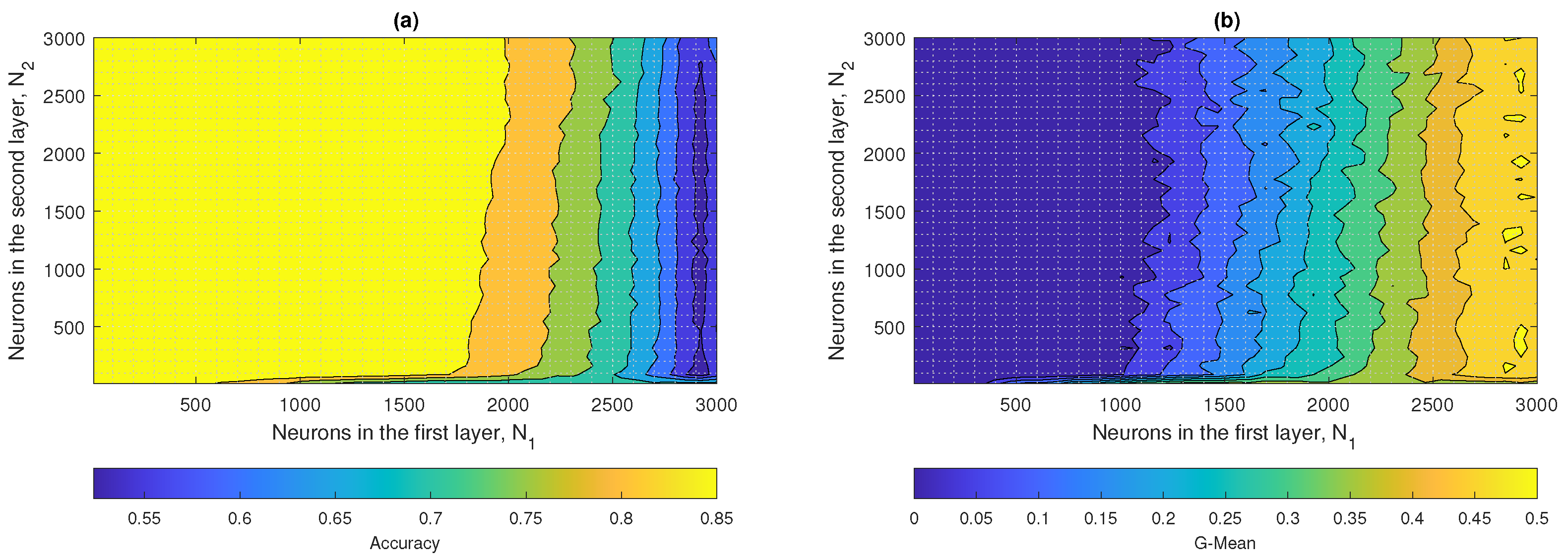
Figure 14a,b show the contour plots corresponding to the accuracy and G-mean values obtained by the ML2-ELM, respectively. In Figure 14a, it was observed that the regions associated with optimal performance were located in the range between $N_1\approx 0$ and $N_2\approx 0$, up to approximately $N_1=1850$ and $N_2=2003$. In turn, in Figure 14b, it was evident that the maximum values of the G-mean were obtained from $N_1\approx 87$ and $N_2\approx 2617$. The hyperparameters that maximized the performance of ML2-ELM were $N_1\approx 2540$ and $N_2\approx 2233$, achieving an accuracy close to 0.73 and a G-mean of approximately 0.43.

4.1.6. Multilayer ELM with Three Hidden Layers

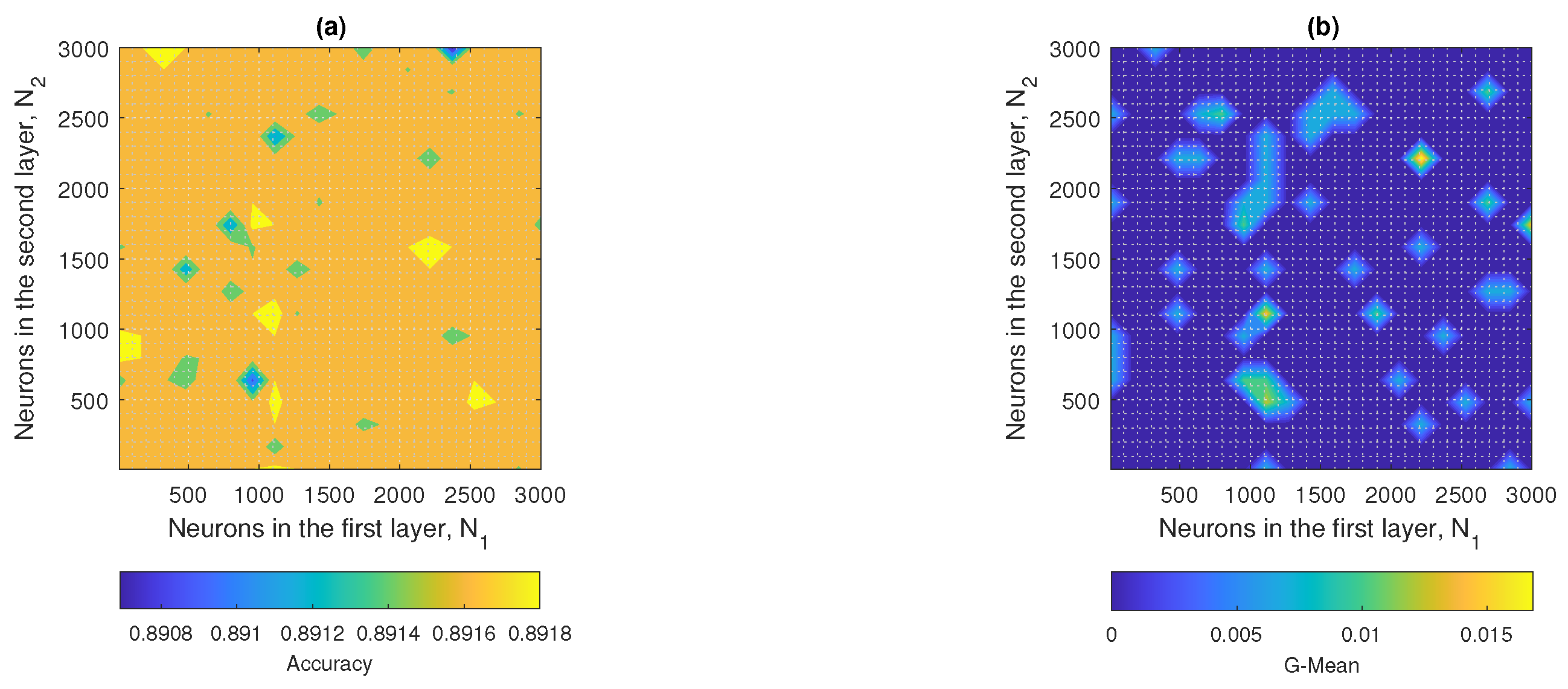
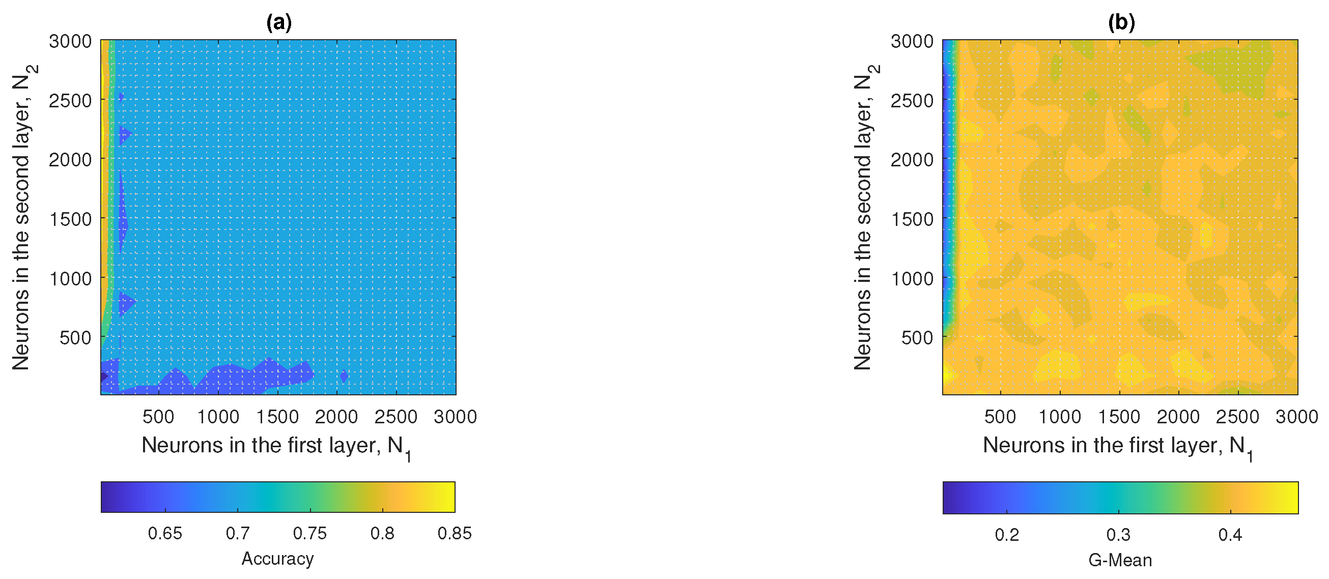
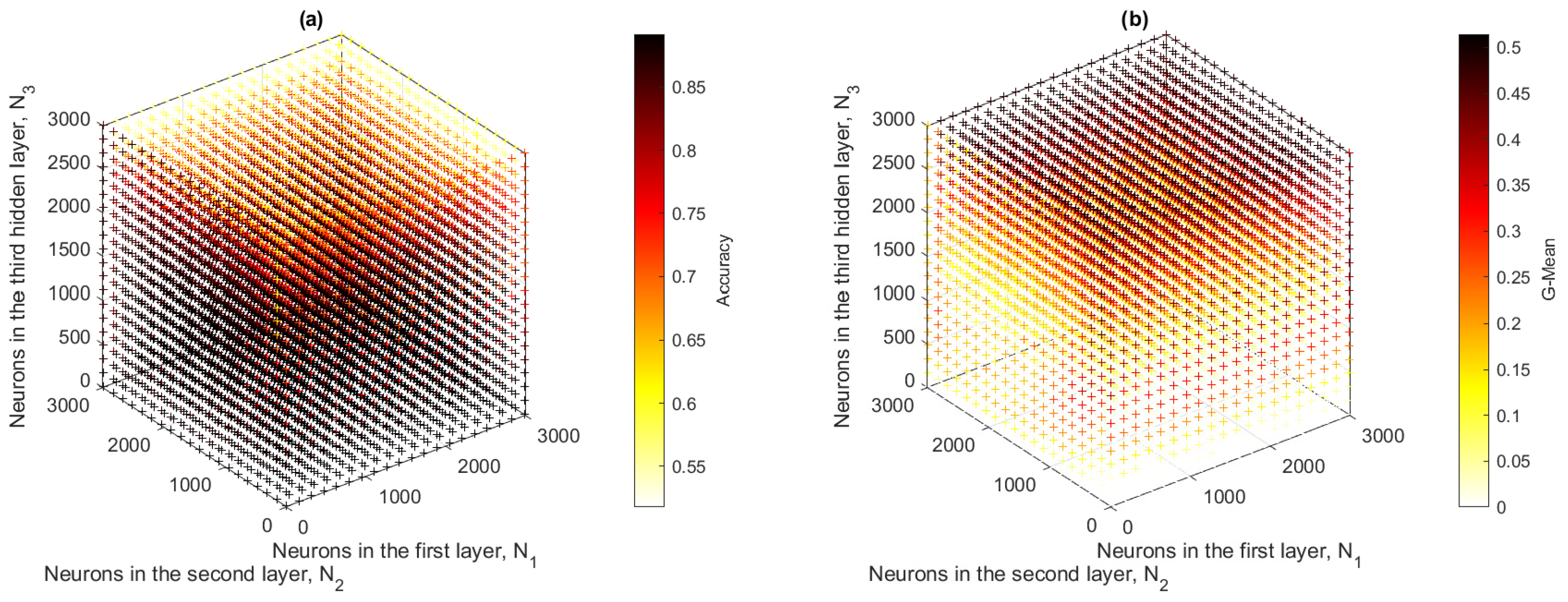
Figure 15a,b show the point clouds corresponding to the accuracy and G-mean values obtained by the ML3-ELM model. Because this model operated in a three-dimensional space, the complete representation of the data made it difficult to accurately visualize the optimal metrics. Therefore, two-dimensional projections were generated by setting different values of the Z axis ($N_3$), which allowed a clearer analysis of the behavior of the metrics. Figure A1 ($N_3=10$), Figure A2 ($N_3=2528$), and Figure A3 ($N_3=3000$) were selected because they provided representative information to identify the optimal model configurations, see Appendix A.

When comparing the results obtained for the different configurations of the parameter $N_3$, it was observed that the model presented contrasting behaviors in terms of accuracy and G-mean. For $N_3=10$, although acceptable accuracy was achieved, the G-mean was extremely low, indicating an inefficient model in classification. In the case of $N_3=3000$, both metrics remained at intermediate values with little variation, without showing a clear maximum point. On the contrary, with $N_3=2528$, a better balance between accuracy and G-mean was achieved, reaching maximum values of 0.72 and 0.43, respectively. These results suggested that the configuration with $N_3=2528$ offered the best compromise between both metrics, being the most appropriate to maximize the performance of the ML3-ELM model on this dataset.

4.2. Analysis and Comparison of Results

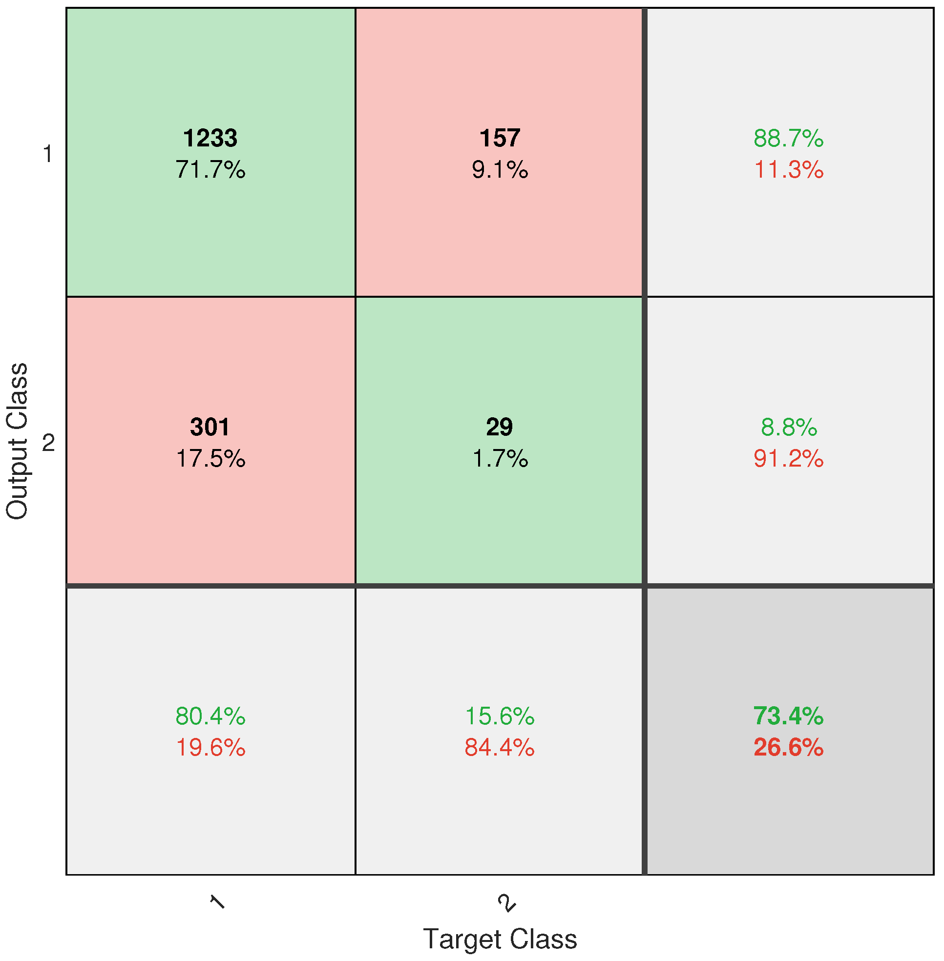
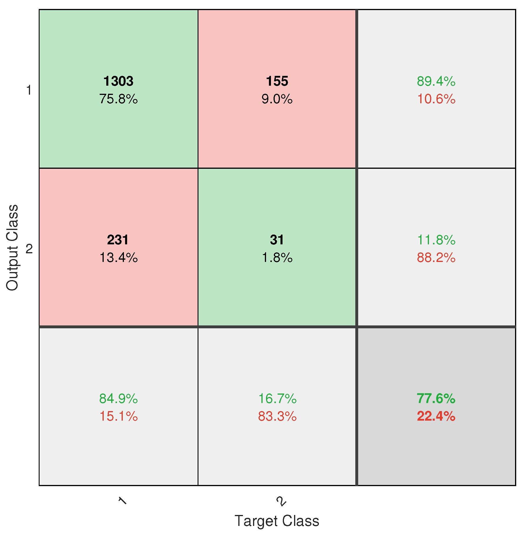
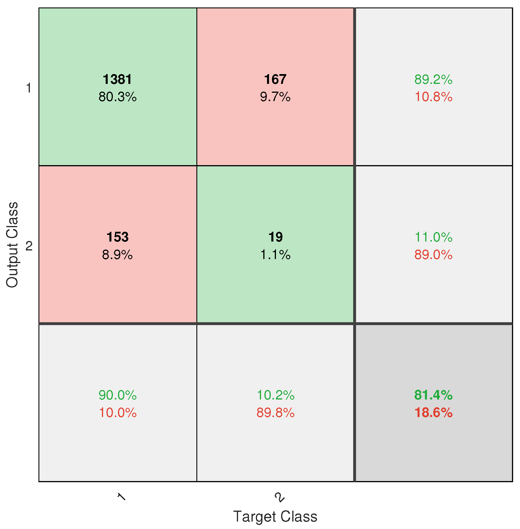
After optimizing the hyperparameters of the different ELM-based algorithms, their performance and complexity (time training, TT expressed in seconds) were compared, as presented in Table 3. In general, the accuracy metric is acceptable although it can be improved to values close to 0.9, the geometric mean must be improved to exceed the value of at least 0.5, and the training times stand out positively, being in the order of seconds. It is important to note that the performance metrics tend to be low, due to the demanding training process considered, that is, the training and testing samples are realistic, since they are from different administrations. Furthermore, the resolution of all images was adjusted (their resolution was normalized) for implementation through a graphical interface, as will be seen in the next section. Among the evaluated models, W2-ELM achieved an accuracy of 0.78 and a G-mean of 0.44. In comparison, the basic ELM model had a high accuracy of 0.86 but a low G-mean of 0.30, suggesting an imbalance toward the majority class, albeit with a good training time. The R-ELM model did not show significant improvements over the baseline model, with similar metrics in accuracy (0.63) and G-mean (0.47). Meanwhile, W1-ELM achieved a G-mean of 0.45 with an accuracy of 0.77. Although both W1-ELM and W2-ELM performed outstandingly, W1-ELM was found to perform the best, outperforming W2-ELM by 0.01 points in G-mean and showing a shorter training time, reflecting greater efficiency. However, although W1-ELM performed the best, its G-mean value is insufficient. Such a low value of G-mean indicates that the model tends to misclassify the minority class (diseased trees), which compromises its usefulness in an unbalanced scenario. Note that the multilayer ELM increases the computational complexity without improving their performance in both accuracy and G-mean. Due to this reason, discussion is excluded. Finally, a visual perspective to see general and particular performance metrics, it is presented in Appendix B by using confusion matrix.

From a computational complexity perspective, standard ELM training is dominated by computing the pseudoinverse of the hidden layer activation matrix. It is well known that this process has a theoretical cost of $\mathcal{O}(m{N}^2+N^3)$, where m is the number of training samples and N the number of hidden neurons [54]. Therefore, although the W1-ELM and W2-ELM models achieve competitive performance in terms of accuracy and G-mean, their main advantage lies in the shorter training time compared to larger or multilayer ELM models, which in practice translates into greater efficiency. This advantage is especially relevant for applications on resource-limited devices, such as mobile phones or embedded systems, where reducing floating-point operations and memory consumption are critical. Therefore, the evaluation of the training time serves as an approximation of the computational complexity and justifies the choice of W1-ELM as a more balanced model.

To expand the comparison between different classification models, the Classification Learner tool in the MATLAB Toolbox was used, unifying the training and test sets into a single file, since the application requires only one input and internally partitions the data. Cross-validation and a 70/30 training/test ratio were used, following the usual recommendations for supervised classification problems [55].

The most representative models available in the tool along with the best proposal (W1-ELM) were evaluated, configuring the default hyperparameters for each one [56]. The results are presented in Table 4, where the models are compared in terms of accuracy, geometric mean (G-Mean), training time (TT), and prediction speed (PS) expressed in observations per seconds.

As can be seen in Table 4, the Cosine KNN emerged as the most balanced model, with high accuracy (0.9285) and G-mean (0.617). Other KNN and SVM models also showed good performance, while neural network models obtained acceptable results, but with lower G-mean values. Naive Bayes algorithms performed less well, and decision trees showed good accuracy, although with limited G-mean. In terms of training times, the Kernel Naive Bayes comes to be the worst approach (858.002 s), while the Fine tree presents the best results (near to the ELM behavior, namely in the order of units of seconds). In order to to the significance for the subsequent application of the models, we can mention that our proposal (W1-ELM) outperforms the rest of the ML approaches since it has the highest number of observations processed per second, namely the minimum time taken for one prediction in seconds.On the contrary, the bilayered neural network shows the inferior prediction speed with only 21 observations per seconds approximately, which means unfeasibility in practice. In this form, W1-ELM exhibits the best performance by considering not only performance but also complexity, in training and testing phases.

Taken together with Table 3 and Table 4, the results confirm that W2-ELM and Cosine KNN were the overall best performing models, while W1-ELM stood out for its significantly reduced training time, making it especially suitable for devices with limited computational capabilities. Although the YOLOv5m model reported in [21] achieved an accuracy of 0.86, W1-ELM offered advantages in efficiency and lower computational complexity, being a practical choice for fast-running applications. Furthermore, the methodology used in [21] is not realistic, since training and testing samples of both years were considered. Due to this, the prediction of Armillaria in cherry trees for a next year cannot be reliable.

Finally, using the previously described methodology, an artificial neural network model was applied, which is a Multilayer Perceptron (MLP) subject to the scaled conjugated gradient as a training algorithm. This as an additional alternative comparison. This model achieved an accuracy of 0.9303, a G-mean of 0.221 and a training time of 48 s, in addition to 7285.453 predicted observations in a single second. Although the MLP presents a higher accuracy than the ELM with better performance, its low G-mean evidences a strong imbalance in the classification, indicating overfitting of the model towards the majority class. In contrast, the ELM maintains higher G-mean in all its models, demonstrating a more balanced behavior between classes. Finally, the MLP is much slower than the ELM as evidenced by its training time and prediction speed. Namely, the MLP cannot be considered in a practical situation, where farmers demand rapid results with not expensive computational equipment.

4.3. Application Development

The application’s user interface was created using the GUIDE tool in MATLAB. This choice facilitated the agile generation and organization of graphical components within the application environment. This application is designed to predict or confirm final diagnoses of Armillaria disease. This is an initial step toward enabling the application’s adoption in embedded systems (such as cell phones) and, consequently, its practical use (cherry plantations).

Figure 16 presents the general workflow of the system, with the stages numbered for a better understanding of the process. It begins in stage 1, with the upload of an image by the user, followed by stage 2, in which the image is preprocessed to prepare the data for subsequent analysis. In stage 3, the system accesses the entire database and randomly shuffles the samples. Then, in stage 4, 62.65% of the data is selected for model training, thus maintaining the same proportion used in the experimental phase. This choice is intended to preserve the methodological consistency of the study. With the selected subset, in stage 5 the ELM-Train (ELM-T) network is trained, generating a dynamically adjusted model in each execution. This decision is due to the fact that the model previously trained during the experimental phase was not reused, given that its purpose was exclusively methodological: to perform simulations and optimize the hyperparameters corresponding to each ELM variant evaluated. Dynamic training seeks to emulate a realistic situation in which, in a future commercial use scenario, a farmer provides a new image, potentially different in terms of lighting, environment, or visual characteristics that have not been previously considered by the system. For this reason, it was decided to generate a new model in each run, using a random subset of the available data. Once training is complete, in stage 6, the weights and biases of the output layer generated by the ELM-T are stored. In stage 7, these parameters are loaded into the ELM-Predict (ELM-P) prediction module, specifically designed to apply these values to the diagnosis of new samples. Finally, in stage 8, the ELM-P model is run to determine whether the tree represented in the input image corresponds to a healthy or diseased specimen. As a result, in step 9, the prediction is displayed directly in the application, thus providing a decision-support tool for the farmer.

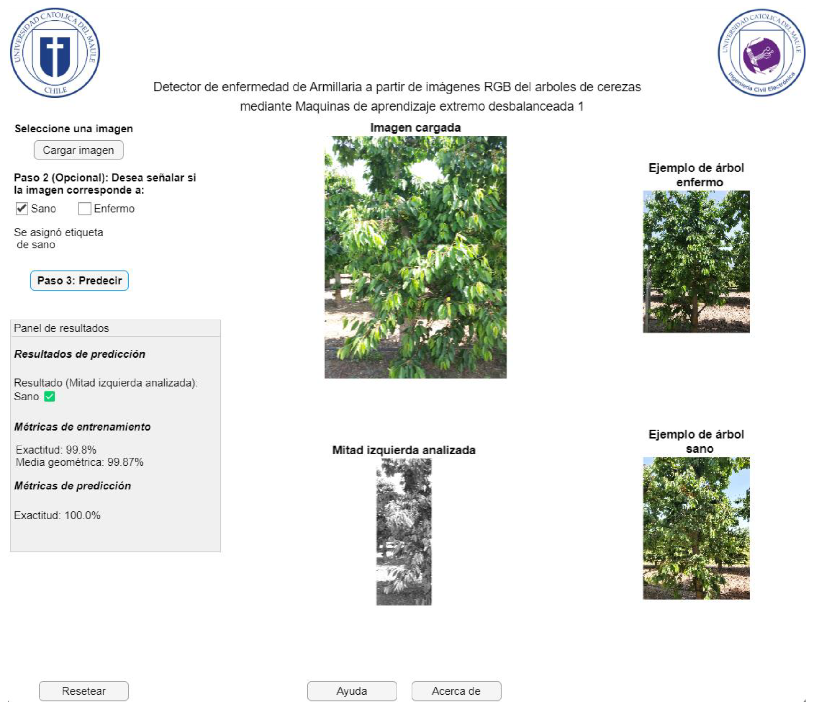
Figure 17 represents the application window of the GUI user interface for detecting Armillaria in cherry trees from RGB images, whose interface is in Spanish, since the software will be disseminated and disseminated in Chile. On this screen, the farmer has the option to upload the image of the sample they wish to analyze (healthy or diseased). They can then select whether the sample is diseased or healthy, or they can directly start analyzing the image. This will process the image and generate the prediction, displaying the result in the corresponding box. The application does not allow progress if the image has not been previously uploaded. Additionally, it is possible to restart the current window, which offers the opportunity to upload a different image. Finally, in case of questions or concerns related to the use of the application, a help window is available that offers support. 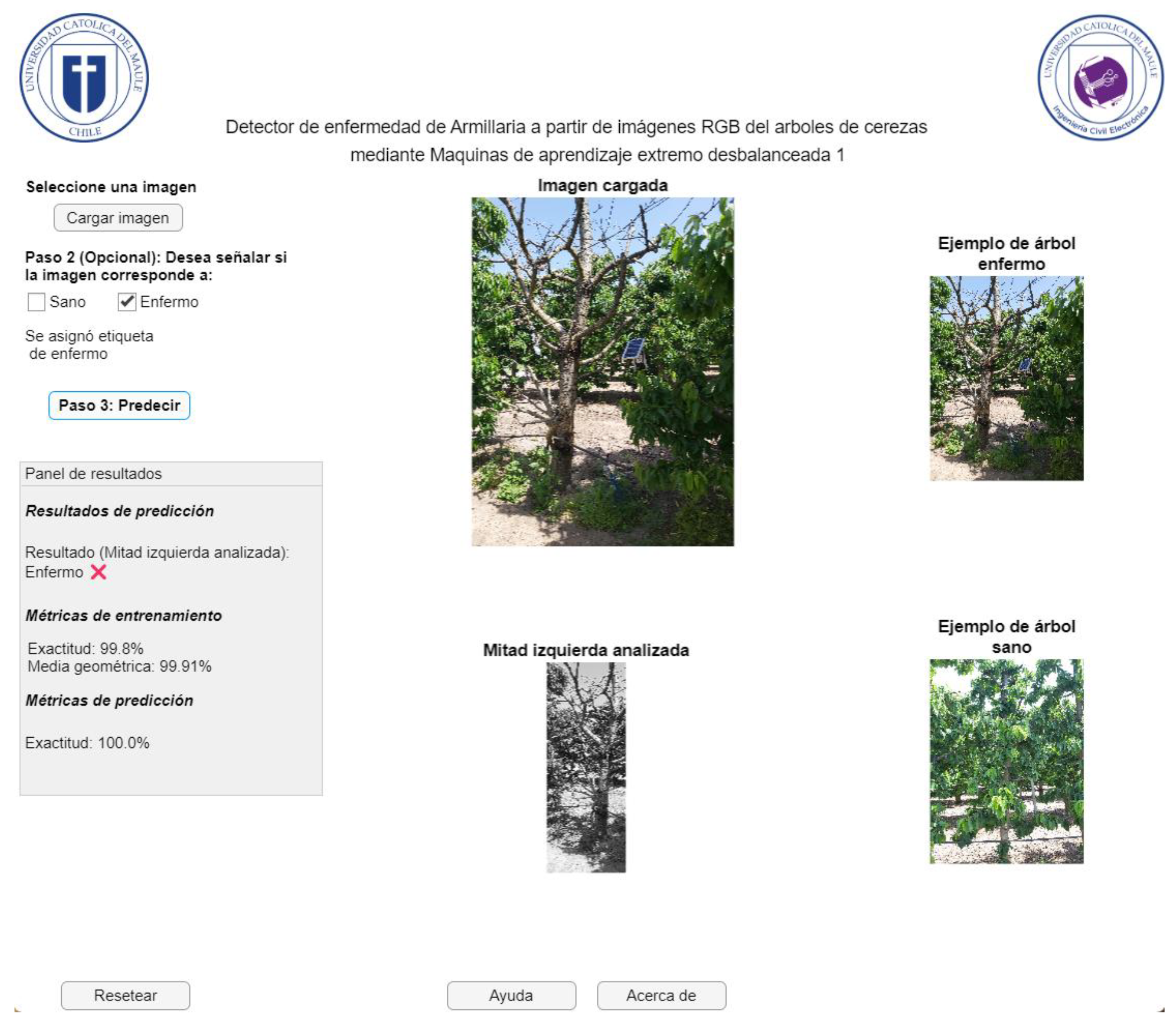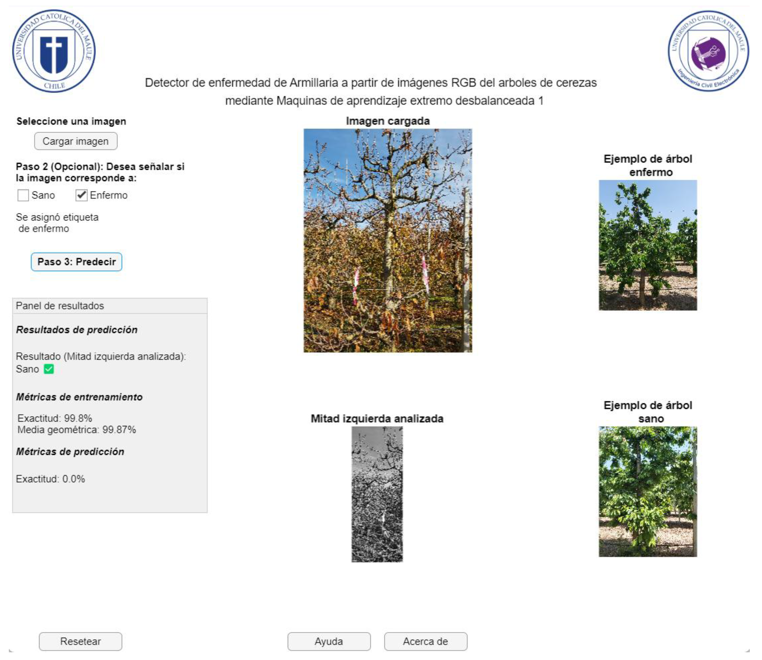In Figure 17, an example of a successful case for the case of healthy trees is shown. In this situation, most of these classes are properly detected (see previous subsection, especially the accuracy metric). In addition, instances of armillaria detection with positive and negative results given by the computational application are presented in Figure 18 and Figure 19, respectively. As expected, these cases are confused for ELM model due to the imbalance degree of the dataset (see section Dataset). This happens despite using an weighted ELM as can be seen in previous outcomes with the G-mean value.

Tests conducted with the application indicate that it is a useful tool, but it has some limitations. Among them, it cannot be used with any RGB image and is highly input-dependent, as the application only supports three dimensions: 3024 × 4032, 1872 × 4160, and 2016 × 4480, since preprocessing is done according to the methodology described above. Furthermore, for the application to function correctly, the computer where it is run must have MATLAB installed. It is worth noting that it can even be used with the free trial version of the software. Ultimately, it makes sense for applications to be constantly updated according to the agronomist’s needs, as small changes can mean days of programming. For example, inputting an RGB image is not the same as inputting a multispectral image. To adapt RGB image processing to multispectral image processing with ELMs, preprocessing and feature extraction must be adjusted. Furthermore, the number of hidden neurons in the ELM must be modified to handle the increased complexity of multispectral imaging. Finally, sensitivity must be prioritized in the assessment to ensure accurate detection of diseased individuals. For this reason, it is difficult to develop a tool that works with any type of image, as numerous factors, such as acquisition method, color space type, and resolution, are involved.

It is worth noting that the application is aimed at farmers and is characterized by its ease of use. It includes an explanatory section on how to use it and how to interpret the results, which can be understood by anyone with primary education. The explanation can be summarized in three steps: first, upload the image to be predicted; second, decide whether to add the label (healthy or diseased); and third, run the prediction option. This tool is helpful for farmers, as it does not increase costs (the farmers themselves can use it) and contributes to increased production (by being able to predict armillaria disease in cherry trees and take appropriate action). The application is not intended to replace the farmer’s work, but rather to serve as a virtual assistant in decision-making and problem-solving related to the health of a plantation. However, it has not yet reached an advanced level of development due to the limitations of the database used: only two years of records are considered, the samples present a significant imbalance, and no data from sensors (objective observations) is available.

Furthermore, there is the option to use the application we are working on without having MATLAB installed. To do so, select the MATLAB Compiler option (a MathWorks tool). This generates an executable file (.exe) that can be installed on any device thanks to the included set of libraries called MATLAB Runtime. Furthermore, MATLAB Compiler not only serves to share applications but also allows them to run without licenses, in various formats, and with code protection.

5. Conclusions and Future Works

This research addresses the need to incorporate artificial intelligence in the agricultural sector, particularly in the early detection of diseases such as Armillaria in cherry trees, a significant threat to export production in the Maule Region, Chile. The hyperparameter tuning results clearly show the impact that class imbalance has on model performance. For example, in Figure A3 it can be observed that the Accuracy exceeds 0.77 in most of the parameterization and even approaches 0.9 in certain configurations. However, in those same regions the G-Mean drops practically to zero, which shows that the classifier fits almost completely to the majority class (healthy trees) and barely manages to recognize the minority class (unhealthy trees). Even under the best training conditions, the G-Mean did not exceed 0.45, confirming that class imbalance is the main limitation to achieving reliable performance. In response to this problem, a computational application was developed in MATLAB based on the W1-ELM variant that offers a very favorable trade-off, with competitive (though not best) performance and superior computational efficiency (training time and prediction speed), using RGB images processed from the ERICA database.

During development, preprocessing processes were implemented and different resolutions were evaluated, determining that 63 × 23 pixels offered the best balance between computational efficiency and performance. Subsequently, six variants of the ELMs model were trained, with the W1-ELM (the best-performing model among the ELM variants tested, but its performance is still insufficient for reliable standalone diagnosis), with an accuracy of 0.77 and a geometric mean of 0.45, positioning it as an efficient option due to low-computational cost.

However, despite the progress made, the application did not achieve completely reliable classification. This is mainly due to the severe class imbalance in the database, with an approximate ratio of 13.2:1 between healthy and diseased trees. Despite the implementation of weighting techniques such as W1-ELM, the results, particularly from the confusion matrix (see Figure A6), show that the model remains biased toward the majority class, with a high rate of positive true and a poor ability to detect positive negative. This limitation directly affects the system’s usefulness as a standalone diagnostic tool.

Even if the system does not require real-time detection, processing speed remains a relevant factor. A low response time allows the worker to obtain almost immediate results, optimizing the effective time dedicated to the inspection and reducing unproductive waiting periods. This is especially important in scenarios with limited computing resources, such as portable devices or field workstations, where a lighter, faster model facilitates implementation without the need for expensive infrastructure. Furthermore, speed increases the system’s scalability, allowing it to process large volumes of data (multiple trees or plots) in less time. However, precision remains a priority, so a balance between speed and accuracy must be sought to ensure that the system delivers reliable results for decision-making.

Therefore, although the application allows for automated predictions accompanied by diagnostic metrics, its use should be understood as a complement to field decision-making, rather than as a definitive diagnostic tool. It is recommended that the results obtained be validated by an expert in the field. In conclusion, the project demonstrates the viability of ELM models as rapid and efficient solutions for classification tasks in agriculture, especially in scenarios with limited computational resources. However, it also underscores the importance of having balanced and representative databases to achieve clinically reliable results.

Beyond its technical contributions, this type of system has direct agricultural relevance in regions highly dependent on fruit production, such as in El Maule, Region in Chile. Implementing a free-license platform would enable farmers to access diagnostic support tools, facilitating early identification of Armillaria in cherry trees. Additionally, incorporating disease severity estimation could enhance decision-making in field management, contributing to reduced economic losses and more sustainable agricultural practices.

In summary, severe class imbalance constitutes the main limitation of this work and limits the reliability of the results. Therefore, the developed application is presented as a support tool that provides speed and low computational cost, but requires validation by a specialist before making important decisions in the field. Its use is appropriate in scenarios with limited technological resources, where it can complement visual inspections and facilitate earlier detection of Armillaria in cherry trees.

Future Works

Additional databases that include abiotic stress factors (drought, nutrient deficiency) could be considered in order to obtain more generalized results, meaning that they can be applied to most cherry plantations. This way, it is possible to anticipate situations beyond our control (due to climate change or poor agriculture) and take early and/or corrective actions to avoid a decrease in cherry production. However, our database does not consider these factors, which presents a limitation and could be considered in future research.

Another area of improvement involves more granular labeling of the dataset, segmenting and classifying individual leaves and branches affected by Armillaria. This strategy would allow models to be trained with greater accuracy and detail, as the disease typically manifests itself locally before affecting the entire tree. This level of labeling has been explored in other studies with good results, such as the YOLOv5 [21] baseline work, but was not implemented in this project due to time and resource constraints. In this sense, it is considered as future work, the comparison in terms of performance and complexity with deep learning approaches (for instance, lightweight CNN or YOLO) with the same methodology (the dataset must be divided by year to prevent future diseases) in order to expose unquestionable outcomes.

Finally, we propose applying advanced image processing techniques to improve the quality of the extracted features before training. This includes noise reduction filtering, edge enhancement, color transformation, or even the use of multispectral images if the appropriate hardware is available. More sophisticated preprocessing could improve visual discrimination between healthy and diseased trees, even under varying lighting conditions, and reduce the model’s dependence on the original image size or quality.