Abstract
The assessment of energy savings is not a trivial matter, as we have direct meters for consumption, but not for the absence of consumption. Calculating a simple difference between consumption before and after the implementation of an energy saving measure is also an incomplete assessment. The only way to determine energy savings is to compare the consumption that would have occurred in the absence of the saving measure with the actual consumption, with reference to the same external conditions and the same period. This is what the international IPMVP® protocol establishes. This study, based on two case studies of industrial energy saving measures, explores the aspects of the calculation related to decarbonization and economic evaluation. In particular, sensitivity analyses of energy and economic indicators are carried out based on factors that evolve over time, such as the rate of inflation and discounting of investments and the variation in the carbon dioxide emission factor for electricity production. The main results highlight that the assumption of a constant electricity emission factor leads to an overestimation of the total CO2 savings from energy efficiency interventions that can be more than 40%. The uniqueness of this paper is the application of a standardized savings evaluation procedure (IPMVP®) in order to analyze the sensitivity of economic savings towards some key financial parameters, and the specific fitting of an electricity emission model to the Italian power sector in order to correct the carbon savings evaluation to the projected emission factor evolution.
1. Introduction
The prioritization of energy efficiency has gradually evolved into a cornerstone of European energy policy. First codified in the Energy Efficiency Directive (EU/2018/2002) [1] and subsequently reinforced by Directive EU/2023/1791 [2], this principle has been operationalized through complementary recommendations of the European Commission [3]. The concept does not only emphasize technical improvements, but requires that efficiency be embedded as a guiding criterion in all planning and investment choices. This, regardless of whether these are directly related to the energy sector. In practice, this translates into methodological frameworks for cost–benefit evaluations that move beyond immediate financial considerations. They explicitly account for societal gains, including environmental sustainability, progress towards climate neutrality, and the fostering of green economic growth. The underlying rationale is that energy systems should be designed to supply only the demand that remains after all feasible efficiency measures have been applied. This reduces both consumption levels and associated costs.
The industrial sector provides several illustrative cases of how efficiency interacts with economic performance [4]. Earlier studies on industrialization dynamics demonstrated that, during the initial phases of economic development, electricity consumption tends to follow economic growth in a one-way relationship. Such findings suggest that restrictive energy policies in these contexts may exert limited influence on GDP. Other research has highlighted that projected returns on energy technologies, such as cogeneration plants [5], often diverge from actual outcomes. Payback periods estimated in the design stages are frequently underestimated, pointing to a systematic bias in investment planning.
Extensive empirical evidence has also been gathered. For instance, Bazzocchi and colleagues [6] examined more than 2500 energy-saving interventions carried out in Italian industries over a decade. They identified those with the highest replicability and estimated the sector-specific potential for energy savings. Their analysis confirmed that the contribution of efficiency to industrial competitiveness depends on both the technical practicability and the economic resilience of the measures implemented.
Parallel developments have taken place internationally. In China, recent studies [7,8] have investigated how efficiency considerations affect capital allocation decisions in industry. Meanwhile, research on residential buildings has proposed integrated design frameworks that balance economic objectives with environmental targets, particularly through insulation and energy-saving strategies [9]. In line with this body of work, the authors of the present study assessed the insulation materials used in Italian buildings using a life cycle perspective [10]. They simultaneously evaluated their impact on reducing energy demand and the embodied energy required for their production. The analysis was complemented by a life cycle cost assessment, thus integrating environmental and economic dimensions. Similarly, Gao and co-authors [11] examined the performance of steam systems in the tobacco industry, showing how the recovery of waste heat from combustion processes could be exploited to provide ancillary thermal services.
More recently, investigations have turned to innovative technological configurations within industrial facilities. One such analysis explored the performance of hybrid heating systems in different Italian climatic zones [12], demonstrating their superior efficiency and cost-effectiveness compared to traditional heating solutions. Another study focused on coupling high-temperature heat pumps [13] with combined cooling, heating, and power systems. The research showed that such hybridization strategies can outperform conventional energy production technologies when assessed across a range of operational parameters.
Aim of the Work and Novelty
The vast majority of the cited studies consider the key financial parameters (interest rate, inflation rate) as fixed in time and kept constant over the analysis period. The same consideration is valid for the energy conversion factor and the energy emission factors. Also, for recent studies is the same. For example, in [14], the authors used Monte Carlo simulations combined with EnergyPlus for assessing energy consumption and indoor thermal comfort in new and retrofitted buildings. Wang et al. [15] determined the path of changing of the operational carbon intensity of commercial buildings since 2000 and, by means of the decomposing structural decomposition method, assessed how electrification impacted the decarbonization of buildings across different countries.
As an overview of building energy estimation methods, different electricity emission factors for estimating operational GHG emissions in whole building life-cycle assessments were analyzed in [16]. At the industry level, Jin et al. [17] analyzed the effect of considering different emission factors, using national, regional, or provincial values, to assess the impact on the carbon accounting results for an electrolytic aluminum industry.
The main aim of this paper is to provide some new approaches for the quantification of savings, both economic and of CO2 emissions, in the long term (i.e., 2050), generated by different interventions in the following:
- scenarios of high inflation rate for energy vectors and sources;
- plausible evolution of carbon dioxide emission factors in electricity conversion.
The determination of energy savings is conducted according to the International Performance Measurement and Verification Protocol (IPMVP®), which has been applied to several real case studies presented herein [18]. The IPMVP® protocol is widely recognized as a formal reference for the measurement and verification of energy savings and explicitly cited in international standards such as ISO 50015:2014 [19]. It constitutes a fundamental methodological framework for Energy Performance Contracts (EPC) as well as for a broad range of other applications [19]. Essentially, the protocol formalizes a logical reasoning process that is often applied intuitively. While energy meters provide accurate measurements of actual consumption, there are no instruments that can directly measure savings. Consequently, savings must be inferred by applying a counterfactual approach. They are defined not as the simple difference between consumption measured in the year preceding the intervention and that recorded in the year following it, but rather as the difference between the hypothetical consumption that would have occurred in the absence of the intervention and the actual consumption observed after its implementation [20]. The conditional nature of this counterfactual baseline is critical, as the specific boundary conditions—such as climatic variations, production schedules, and operational factors—govern the methodological approach to the calculation of savings. In practice, the evaluation involves a comparison between pre- and post-intervention energy consumption, with appropriate normalization and adjustments to account for any variations in these influencing conditions (Figure 1).
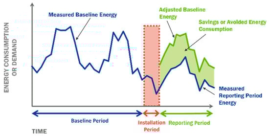
Figure 1.
Determination of energy savings according to the IPMVP® protocol (courtesy of the Efficiency Valuation Organisation).
2. Materials and Methods
2.1. Economic and Financial Parameters
Calculating energy and economic savings is a fundamental step in monitoring the effectiveness of the implemented energy efficiency measures over time. A critical aspect that is often overlooked in such analyses concerns the temporal variability of the parameters that were assumed to remain constant during the intervention design phase. In practice, these parameters may exhibit significant fluctuations in the medium term, potentially affecting both the actual performance of the measures and the accuracy of the savings assessment.
From an economic standpoint, considerations apply to the monetization of energy savings. For an identical quantity of electricity saved, an increase in the national single price (Prezzo Unico Nazionale, PUN) entails a substantial amplification of the corresponding economic value (Figure 2). As an illustrative example, the financial evaluation of an investment in electricity savings conducted using end-2021 prices (approximately 80 EUR/MWhe) was subsequently reassessed in markedly positive terms following the unprecedented escalation in electricity prices observed in 2022, when the average PUN reached 543 EUR/MWhe in August (due to the post-pandemic economic recovery and the energy crisis triggered by the war in Ukraine). This exceptional market dynamic produced significant—and in some cases severe—financial consequences for Energy Performance Contracts (EPC) indexed to the PUN. Although this surge had been qualitatively anticipated, its quantitative magnitude was extraordinary and is unlikely to be replicated in the short term. Nevertheless, analogous phenomena have occurred elsewhere: California, for instance, experienced in 1999 a comparable event—albeit driven by different structural factors—when the functional equivalent of the PUN exceeded 1000 USD/MWhe. Such developments, therefore, cannot be excluded a priori. The subsequent sections, through the analysis of two representative case studies, seek to underscore the methodological and interpretative caution required when applying economic and financial evaluation techniques to assess the cost-effectiveness of energy efficiency interventions under conditions of high price volatility.
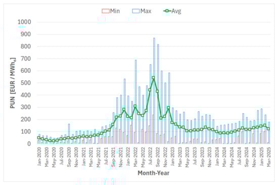
Figure 2.
Monthly average, maximum, and minimum PUN values from January 2020 to March 2025 (data from https://gme.mercatoelettrico.org/it-it (accessed on 15 April 2025)).
2.2. Emission Factor
As an illustrative example, Figure 3 reports the carbon dioxide emission factor associated with electricity use (i.e., referred to final consumption), based on data from an institutional source [21]. Between 2007 and 2012, this factor decreased from 455.3 to 374.3 kgCO2/MWhe, corresponding to a reduction of approximately 18%. A further decline was recorded between 2018 and 2023, from 282.1 to 236.3 kgCO2/MWhe (−16%). This sustained downward trajectory of emission factors implies that, for an equivalent reduction in electricity consumption, the long-term environmental effectiveness of energy efficiency measures—expressed in terms of avoided CO2 emissions—tends to diminish over time. This dynamic underscores the importance of considering prospective changes in the electricity mix when assessing the environmental benefits of energy efficiency interventions.
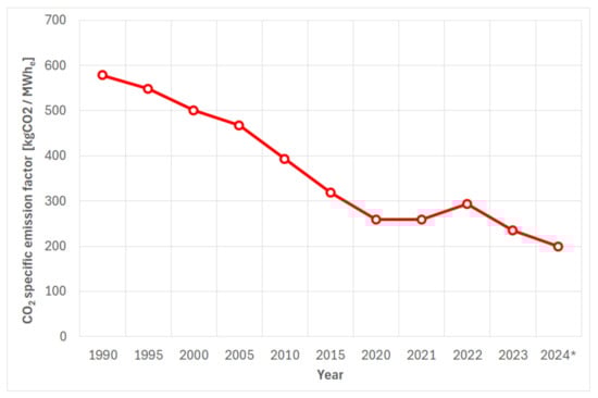
Figure 3.
CO2 emission factor for electricity consumption in Italy (* data for 2024 are not definitive [21]).
Most of the literature on the case study considers the value of the emission factor as the one scored by the national electric system in the current year of implementation of the energy efficiency measure. However, the previous graph suggests that a progressive reduction in the electricity carbon factor trend should be taken into account.
Recent papers start a new perspective on accounting for variability in carbon emissions in electricity generation [22], with some special reference to buildings [23]. Some studies eventually also focused on the evolution of carbon factors and electricity markets [24] and towards climate-neutral energy systems [25].
The approach provided in this paper is the one proposed by the Myopic transition path [26]. The myopic code can be employed to analyze progressive structural changes within an energy system network, such as those occurring along a decarbonisation or transition pathway. In this modeling framework, the capacities installed at each time step remain in operation until the end of their respective technical lifetimes, enabling a dynamic representation of infrastructure turnover over time. The myopic approach was originally developed and applied [27] and was subsequently refined and extended [28].
It should be noted that the Myopic model faces some limitations, since it cannot account for energy crisis or sudden policy changes; however, a careful application of the model can give some new perspective to read current emission savings data and project them into the future. It should also be reminded that there is correlation by industry sectorial development and a country’s CO2 trajectory [29]. The current implementation adheres to the standard workflow and ensures compatibility with the high-resolution electricity transmission model, thus allowing for analyses that go beyond simplified representations of one-node-per-country. From this well known model, the equation of the emission factor e(t) over time t can be written as follows (Equation (1)):
where
- e0 is the emission factor of the first year of operation;
- r is the initial linear growth rate, which is assumed here to be r = 0;
- m is the decay parameter.
The decay parameter can be calculated by imposing the integral of the path to be equal to the budget for Europe (or the specific State) or by a easier “fit” over the past data.
The Myopic model variables are t (time, independent variable) and e(t), the emission factor at time t (dependent variable). Parameters r and m are determined as follows: r (initial growth rate) is imposed to a value of 0 (assumption) by looking at the diagram or a possible fit to the statistical data for Italy; m is calculated via “fittings” with nonlinear regression, as it is written in the text. With respect to the value of “m”, it is also possible to calculate it by integrating the formula into the specific State carbon budget. Since this last value of the carbon budget also changes in time according to environmental policies (ratification or amendments of international treaties), it was chosen to adopt a simpler approach, i.e., to fit the model backwards.
For the sake of discussion, the previous formula can also be “symbolically” integrated and the result is the following Equation (2):
and with r = 0 (Equation (3)):
However, this last expression will not be used in the paperwork.
The application of the Myopic model to the Italian electric system that was applied in this work is quite simple and follows the rule of a regression (nonlinear). In this way, the regression can be handled alternatively:
- with e0 = initial value of the historical series (e(1990)), least squares approximation on m only, called “model opt(e0 = e(1990))”;
- least squares approximation on both e0 and m, called “model opt”.
The results are shown in Figure 4.
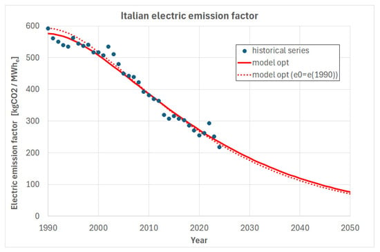
Figure 4.
Two possible fits for the Myopic model to the Italian electric system (own research).
The results of the fit are summarized in the following Table 1, including the value of R2. The main result of the fit is the decay coefficient “m”.

Table 1.
Coefficients of the fit (own research).
2.3. The Case Studies
The determination of energy savings according to the IPMVP® protocol can be performed using four alternative methodologies:
- A.
- isolation of the intervention with measurement of the main parameters;
- B.
- isolation of the intervention with measurement of all parameters;
- C.
- assessment of the entire plant or structure based on pre- and post-intervention measurements;
- D.
- assessment of the entire plant or structure based on post-intervention measurements combined with a calibrated pre-intervention simulation.
The two case studies presented concern:
- Case 1. A company operating in the wooden office furniture sector, located in the Province of Padova (North-East Italy). The analysis focuses on the energy savings achieved through a substantial modification of the production processes. In particular, the assembly line was restructured by replacing both the die-cutting machine (Figure 5) and the packaging line (Figure 6), representing an intervention that combined technological upgrading with managerial reorganization. The project was implemented within the framework of the POR FESR 2014–2020 regional funding program (Veneto Region), specifically under the call addressing the “replacement of production cycles with cycles that demonstrably reduce electrical and/or thermal consumption compared to the pre-intervention situation, including per unit of product.” As the company did not have a detailed energy monitoring system in place, IPMVP® Option C was selected for the determination of savings, relying on pre- and post-intervention energy consumption data at the level of the entire plant. The pre-intervention baseline period was defined as the entire year 2019, while the reporting period for the calculation of savings corresponded to the entire year 2021. Two energy audits were carried out according to the ENEA protocol pursuant to Legislative Decree 102/2014 [16], one referring to the baseline year (2019) and the other to the reporting year (2021). The energy data used in the analysis derive from the processing and results of these two audits.
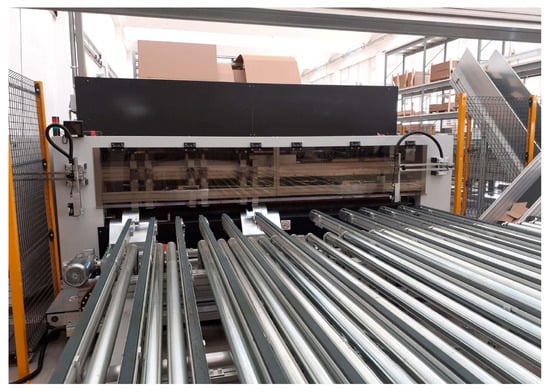 Figure 5. The new die-cutting machine (Case 1—own research).
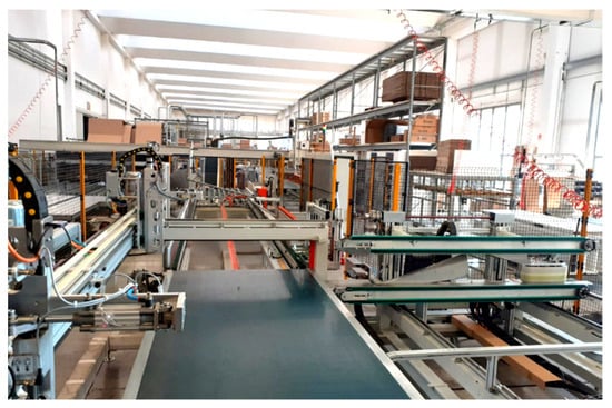 Figure 6. Part of the newly installed packaging line (Case 1—own research).
 - Case 2. A company that operates in the sheet metal cutting and bending, in the same Province of Padova. The analysis focuses on the reduction in electricity consumption due to the installation of a new laser-cut machine that replaces two different machines for metal cutting and punching, which can be seen in Figure 7. The energy efficiency project is developed under the Italian national framework Industry 5.0 for industrial automation and energy saving. Also this second company is not equipped with energy monitoring, but IPMVP® Option A was selected for the determination of savings, relaying on field measurement of the old machines and the new machine consumption when the same production schedule runs in parallel.
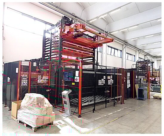 Figure 7. Part of the newly installed laser-cut machine (Case 2—own research).
3. Results and Discussion
3.1. Evaluation of Savings—Case 1
The results of the intervention in Case 1 are summarized in Table 2. The energy savings S were determined according to the following Equation (4):
where
Table 2.
Energy and CO2 emissions results summary—Case 1 (own research).
S = energy savings;
Eref = energy consumed during the reference period
Erep = energy consumed during the reporting period;
adjustments = appropriate adjustments for changes in conditions.
Adjustments were carried out using the backcasting technique, whereby the energy consumption of the reporting period is adapted to the boundary conditions of the baseline period. In the present case study, the adjustment factor corresponds to the production output, expressed in terms of mass (kg). The data collection method is the simple total consumption of the factory, by its energy (electricity and gas) bills. Accordingly, the energy savings equation can be reformulated as follows (Equation (5)):
where
Eadj,2021 = energy consumed during the reporting period (2021) adjusted;
Erep,2021 = energy consumed during the reporting period (2021);
Qproduct,2021 = quantity of product during the reporting period (2021);
Qproduct,2019 = quantity of product during the reference period (2019)
The primary energy conversion factors adopted for the analysis were as follows:
- 0.187 × 10⁻³ toe/kWhe;
- 8.250 × 10⁻⁷ toe/Sm3;
- 11,630 kWh/toe.
With regard to electricity, the reduction in consumption achieved through the intervention was significant both in relative terms (−57%) and in absolute terms (1476 MWhe compared to 1630 MWhe). Overall, the intervention resulted in a 54% reduction in non-renewable primary energy consumption per unit of production. It is noteworthy that, in the absence of the backcasting adjustment, the calculated reduction would have been limited to only 3.4%, highlighting the critical role of the adjustment procedure in accurately assessing the achieved savings.
3.2. Evaluation of Savings—Case 2
Since the intervention provides that the new laser-cut machine (Figure 7) will replace the old cutting machine and the punching machine, the savings can be calculated by determining the specific consumption of the existing machines per each manufactured item and that of the new laser-cut machine: the difference in the specific consumption multiplied by the number of machined items gives the amount of savings (Equation (6)).
where
SCold = Specific Consumption of the old machines (kWhe/item);
SCnew = Specific Consumption of the new machine (kWhe/item);
#item = number of items manufactured in a year (#);
The results of the measurements during one test are summarized in Table 3, showing the beginning and the end of the measurement, the number of machined items, the electric consumption of the machine(s) and the specific consumption.
Table 3.
Summary of results of energy and CO2 emissions—Case 2 (own research).
The number of items (#) produced in 2024 is 28,762, and the conversion factors are the same as for Case 1. Case 2 infers the saving on the full year 2025 (for which the data—of course—cannot be complete), by assuming the same # of items as in 2024.
Therefore, the savings from the new laser-cut machine will be 4316 kWhe/year.
3.3. The Impact of Variation in Economic Parameters
As in the previous section, the following analysis focuses on electricity consumption. A similar discussion could be conducted for natural gas; however, the lack of hourly load curve data limited the scope of the present investigation. The particularly dynamic period in terms of energy price fluctuations (Figure 8) raises two additional research questions:
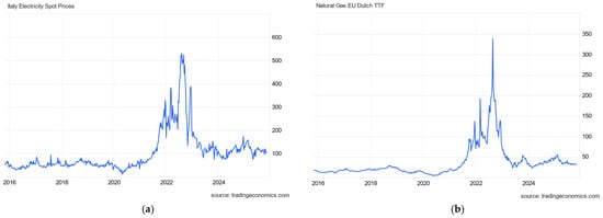
Figure 8.
Italy Electricity Spot Prices (EUR/MWhe) (a) and Natural Gas EU Dutch TTF (EUR/MWhp) (b) (updated to 5 March 2025).
- (i)
- to what extent a sustained increase in energy prices amplifies the calculated economic savings; and
- (ii)
- to what extent inflation (Figure 9) affects the actual profitability of energy efficiency investments.
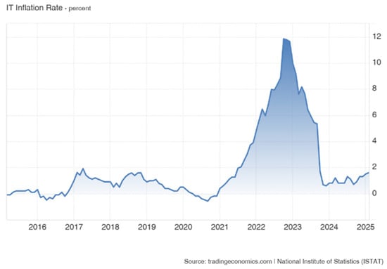 Figure 9. Inflation rate in Italy during the last 10 years (Source tradingeconomics.com) updated to 5 March 2025).
Inflation can typically be neglected in economic assessments when its rate is lower than the discount rate applied in the evaluation of cash flows (e.g., for Net Present Value (NPV) calculations). However, during periods of high inflation, it must be explicitly incorporated into the investment analysis [30]. In Figure 9, it is apparent that the peak in inflation in 2022 was mainly due to the increase in energy prices, due to the post-pandemic economic recovery and the energy crisis triggered by the war in Ukraine. In 2023, average inflation decreased significantly, thanks mainly to the drop in energy prices.
The first key parameter to consider is the interest rate, which represents the time value of money and is conceptually independent of inflation. Among all parameters involved in economic analyses, it is arguably the most strongly influenced by subjective judgment and contextual uncertainty. Its magnitude depends on several factors, including the following:
- -
- the type of subject undertaking the investment (e.g., private individual, public administration, company with high or low profit margins);
- -
- the source of capital;
- -
- the company’s financial strategy and profit expectations.
The interest rate can vary considerably, from values close to those of government bond yields (approximately 3–4%) to substantially higher figures (up to 20%). For this reason, when available, the Weighted Average Cost of Capital (WACC) is often adopted as a reference, acknowledging that it is itself time-dependent and should be periodically updated during the monitoring and revision of investment projects. Ultimately, the interest rate used in the analysis should be representative of the Minimum Attractive Rate of Return (MARR).
Conversely, inflation reflects the erosion of the purchasing power of money over time, linking cash flow values expressed in current terms (i.e., nominal monetary values exchanged in the year of reference) to those expressed in constant terms (i.e., real monetary values referenced to a specific base year, such as year “0,” when the energy efficiency investment is undertaken). In this context, the nominal or monetary interest rate (im) establishes the equivalence between cash flows occurring in different years, whereas the inflation rate (b) quantifies the temporal change in purchasing power. The relationship between these two rates enables the derivation of the real interest rate (ir), which reflects the time value of money net of inflation. This conversion is expressed by the following Equation (7):
According to the O–ML–P (Optimistic—Most Likely—Pessimistic) scenario analysis technique, three alternative trajectories for the average annual inflation rate of energy prices were defined to evaluate future electricity expenditure savings:
- -
- O (Optimistic): 9% per year;
- -
- ML (Most Likely): 6.7% per year, corresponding to the average electricity price inflation observed between 2005 and 2015;
- -
- P (Pessimistic): 4% per year.
As expected, higher inflation rates correspond to higher projected energy prices and, consequently, to greater economic savings associated with reduced electricity consumption.
It is instructive to examine how different combinations of monetary interest rates and inflation rates affect investment profitability when cash flow discounting is performed using the real interest rate, derived from the combination of nominal interest and inflation. Two boundary values were selected for the monetary interest rate im (4% and 20%), and three representative values for the general inflation rate b (3%, 8%, and 15%). Table 4 and Table 5 report the Net Present Value (NPV)—calculated as the sum of all discounted cash flows—for the Most Likely (ML) scenario across all possible (b, im) pairs.
Table 4.
Possible scenarios for the NPV (€) of savings—Case 1 (own research).
Table 5.
Possible scenarios for the NPV (€) of savings—Case 2 (own research).
As expected, the variation in these parameters produces a wide divergence in the resulting NPV. Specifically:
- -
- the case characterized by low inflation and high interest (b = 3%, im = 20%) leads to a marked reduction in the present value of future cash flows;
- -
- the case with moderate inflation and low interest (b = 8%, im = 4%), corresponding to a negative real interest rate, yields a substantially higher NPV;
- -
- the pairs (b = 3%, im = 4%) and (b = 15%, im = 20%), while numerically proportional, produce similar but not identical results due to the nonlinear relationship between nominal interest, inflation, and the derived real interest rate.
3.4. The Impact of the Evolution of the Electricity Emission Factor
Regarding the savings in CO2 emissions, since the intervention of Case 1 was implemented in 2020 and that of Case 2 in 2025, different calculations were performed. The CO2 savings are accounted for in the future period. Case 1 was implemented in 2020; its initial CO2 saving was calculated with the emission factor of 2020. Case 2’s initial savings are calculated with an emission factor of 2025 (estimated by the Myopic model). In both cases, CO2 savings in the years following the implementation are estimated with emission factors calculated from the Myopic model. The cumulative savings from the year of the implementation of the energy efficiency measures until 2050 were calculated in three different scenarios:
S0, with a constant electricity emission factor and equal to that of the year of implementation, 280.5 gCO2/kWhe in 2020, 240.5 gCO2/kWhe in 2024;
S1, with a variable electricity emission factor, considering the “model opt” of Table 1;
S2, with variable electricity emission factor, considering the model with e(0) = e(1990) in Table 1.
The results of the comparison can be appreciated in Figure 10 and Figure 11, while those of the cumulative CO2 emissions are summarized in Table 6.
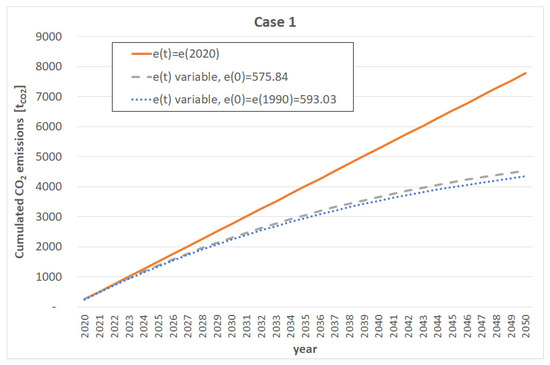
Figure 10.
Cumulative CO2 emission savings—Case 1 (own research).
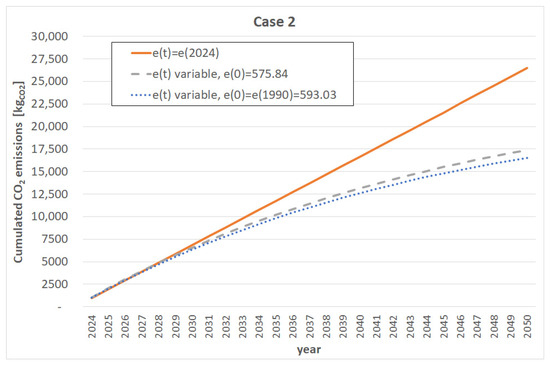
Figure 11.
Cumulative CO2 emission savings—Case 2.
Table 6.
Comparison of the cumulative emissions (from the year of the implementation of the energy efficiency measures until 2050) scenarios (own research).
As it comes out from plots and the Table, the assumption of a constant electricity emission factor leads to an impressive overestimation of the total CO2 savings from the energy efficiency interventions.
At the same time, the difference in cumulative values between the two different evolution models explained in Table 1 is very low, less than 5%.
As of at the European level, Italian energy policies have evolved in a sort of acceleration, especially in terms of electricity generation and its emission factor, over the last three decades, the current target is 65% renewables in 2030. That is why it is very important to develop this kind of projection.
4. Conclusions
In periods of elevated inflation, it becomes essential to conduct a thorough assessment of cash flows, taking into account the combined effects of inflation and interest rates. This introduces a critical additional component to the economic analysis of energy efficiency investments. The cases examined clearly illustrate that the assumptions commonly adopted in recent years—such as stable interest rates and negligible inflation—can no longer be considered valid without careful scrutiny, and must be reassessed to ensure the robustness and reliability of the economic evaluation. In the two case studies here analyzed, the case characterized by low inflation and high interest (β = 3%, im = 20%) leads to a NPV of future cash flows that is between 1/4 and 1/3 of that of the case characterized by high inflation and low interest (β = 15%, im = 4%).
With respect to greenhouse gas emissions, a new perspective on CO2 savings generated from energy efficiency measures is opened by considering the possible evolutions of the electric system. The progressive reduction in electricity emission factors, if not taken into account, could eventually lead to an overestimation of the carbon dioxide savings (which, in the case studies here analyzed, is in the range of 34–44% depending on the scenario considered) and of the profitability of the economic investment.
Author Contributions
Conceptualization, F.B. and M.N.; methodology, F.B. and M.N.; validation, F.B.; data curation, F.B.; writing—original draft preparation, F.B. and M.N.; writing—review and editing, F.B. and M.N. All authors have read and agreed to the published version of the manuscript.
Funding
This research received no external funding.
Institutional Review Board Statement
Not applicable.
Informed Consent Statement
Not applicable.
Data Availability Statement
The original contributions presented in this study are included in the article. Further inquiries can be directed to the corresponding author.
Acknowledgments
The authors thank Roberta D’Orazio (Innovation manager) and Caccaro srl (Villa del Conte, Padova) for the data provided.
Conflicts of Interest
The authors declare no conflicts of interest.
Nomenclature
| Symbol | Meaning | Unit |
| b | Inflation rate | - |
| E | Electrical energy consumed | kWhe |
| e | Emission factor | kgCO2 kWhe−1 |
| i | Interest rate | - |
| m | Decay parameter | - |
| Q | Quantity of product | - |
| r | Initial linear growth rate | - |
| S | Energy savings | kWhe |
| SC | Specific consumption | kWhe item−1 |
| t | Time | h or y |
| Subscript | Meaning | |
| 0 | Initial value | |
| e | Electricity | |
| m | Monetary | |
| new | New machine | |
| old | Old machine | |
| p | Primary energy | |
| product | Product | |
| r | Real | |
| ref | Reference period | |
| rep | Reporting period | |
| tot | Total | |
| Acronym | Meaning | Unit |
| ENEA | Agenzia nazionale per le nuove tecnologie, l’energia e lo sviluppo economico sostenibile (Italian National Agency for New Technologies, Energy and Sustainable Economic Development) | - |
| EPC | Energy Performance Contract | - |
| EU | European Union | - |
| GDP | Gross Domestic Product | EUR |
| GHG | GreenHouse Gases | - |
| IPMVP | International Performance Measurement and Verification Protocol | - |
| MARR | Minimum Attractive Rate of Return | - |
| ML | Most Likely | - |
| NPV | Net Present Value | EUR |
| O | Optimistic | - |
| P | Pessimistic | - |
| PUN | Prezzo Unico Nazionale (National Single Price) | EUR kWhe−1 |
| WACC | Weighted Average Cost of Capital | - |
References
- European Commission. Directive (EU) 2018/2002 of the European Parliament and of the Council of 11 December 2018 Amending Directive 2012/27/EU on Energy Efficiency; European Commission: Brussels, Belgium, 2018. [Google Scholar]
- European Commission. Directive (EU) 2023/1791 of the European Parliament and of the Council of 13 September 2023 on Energy Efficiency and Amending REGULATION (EU) 2023/955 (Recast); European Commission: Brussels, Belgium, 2023. [Google Scholar]
- European Commission. Commission Recommendation (EU) 2021/1749 of 28 September 2021 on Energy Efficiency First: From Principles to Practice—Guidelines and Examples for Its Implementation in Decision-Making in the Energy Sector and Beyond; European Commission: Brussels, Belgium, 2021. [Google Scholar]
- Liu, L.; Ma, X.Q.; Mao, Z.J. Empirical study on the economic effect of energy conservation and emission reduction in different industrial stages. Adv. Mater. Res. 2014, 962–965, 1541–1546. [Google Scholar] [CrossRef]
- Badami, M.; Camillieri, F.; Portoraro, A.; Vigliani, E. Energetic and economic assessment of cogeneration plants: A comparative design and experimental condition study. Energy 2014, 71, 255–262. [Google Scholar] [CrossRef]
- Bazzocchi, F.; Borgarello, M.; Gobbi, M.E.; Businge, C.N.; Realini, A.; Zagano, C.; Maggiore, S. L’Efficienza Energetica Nell’Industria: Potenzialità di Risparmio Energetico e Impatto Sulle Performance e Sulla Competitività Delle Imprese (In Italian: Energy Efficiency in Industry: Potential for Energy Savings and Its Impact on Business Performance and Competitiveness). RSE Report. 2018. Available online: https://fire-italia.org/wp-content/uploads/2019/07/doc_doc_18001189-318177.pdf (accessed on 4 August 2025).
- Guo, Q.; You, W. Decoupling analysis of economic growth, energy consumption and CO2 emissions in the industrial sector of Guangdong Province. Int. J. Low-Carbon Technol. 2023, 18, 494–506. [Google Scholar] [CrossRef]
- Wu, M. The impact of eco-environmental regulation on green energy efficiency in China—Based on spatial economic analysis. Energy Environ. 2023, 34, 971–988. [Google Scholar] [CrossRef]
- Shen, T.; Sun, L. Evaluating Energy Efficiency Potential in Residential Buildings in China’s Hot Summer and Cold Winter Zones. Int. J. Heat Technol. 2023, 41, 1468–1478. [Google Scholar] [CrossRef]
- Lazzarin, R.M.; Busato, F.; Castellotti, F. Life cycle assessment and life cycle cost of buildings’ insulation materials in Italy. Int. J. Low-Carbon Technol. 2008, 3, 44–58. [Google Scholar] [CrossRef]
- Gao, W.; Zuo, X.; Liu, X.; Yan, L.; Pang, J.; Qiao, W.; Xu, X.; Liang, Y.; Bu, Y. Energy Efficiency Analysis and Energy-Saving Measures for the Steam System in a Cigarette Factory in Zhangjiakou. Int. J. Heat Technol. 2024, 42, 1173–1184. [Google Scholar] [CrossRef]
- Noro, M.; Mancin, S.; Cerboni, F. High efficiency hybrid radiant and heat pump heating plants for industrial buildings: An energy analysis. Int. J. Heat Technol. 2022, 40, 863–870. [Google Scholar] [CrossRef]
- Noro, M. High temperature heat pump with combined cooling, heat and power plant in industrial buildings: An energy analysis. Int. J. Heat Technol. 2023, 41, 489–497. [Google Scholar] [CrossRef]
- Algburi, S.; Mohammed, A.; Abdullah, I.; Hanoon, T.M.; Fakhruldeen, H.F.; Mukhitdinov, O.; Jabbar, F.I.; Hassan, O.; Khudhair, A.; Kato, D. Predictive modeling of building energy consumption and thermal comfort for decarbonization in construction and retrofitting. Results Eng. 2025, 26, 105475. [Google Scholar] [CrossRef]
- Wang, T.; Ma, M.; Zhou, N.; Ma, Z. Toward net zero: Assessing the decarbonization impact of global commercial building electrification. Appl. Energy 2025, 383, 125287. [Google Scholar] [CrossRef]
- Greer, F.; Raftery, P.; Horvath, A. Considerations for estimating operational greenhouse gas emissions in whole building life-cycle assessments. Build. Environ. 2024, 254, 111383. [Google Scholar] [CrossRef]
- Jin, Y.; Xu, S.; Guo, Q.; Xiong, N. Analysis of the Impact of Electricity Emission Factor Selection on High Energy-Consuming Industries under the National Carbon Market Expansion. In Proceedings of the 4th International Conference on Energy Power and Electrical Engineering Epee 2024, Wuhan, China, 20–22 September 2024; IEEE: Piscataway, NJ, USA, 2024; pp. 1050–1053. [Google Scholar] [CrossRef]
- EVO. IPMVP 2016 Basic Concepts. 2016. Available online: https://evo-world.org/en/ipmvp-current/ipmvpcore-concepts/1754-2016-ipmvp-core-concepts-in-italian/file (accessed on 4 August 2025).
- ISO 50015:2014; Energy Management Systems—Measurement and Verification of Energy Performance of Organizations—General Principles and Guidance. ISO: Geneva, Switzerland, 2014.
- Bruni, G.; De Santis, A.; Herce, C.; Leto, L.; Luciani, S.; Martini, C.; Martini, F.; Tocchetti, F.A.; Toro, C.; Salvio, M. L’Obbligo Di Diagnosi Energetica AI Sensi Dell’Art. 8 Comma 1 E 3 Del d.lgs. 102/2014: Le Risultanze Dell’Adempimento Normativo Alla Scadenza Del Dicembre 2020 (In Italian, “The Energy Audit Requirement Pursuant to Article 8, Paragraphs 1 and 3 of Legislative Decree 102/2014: The Results of Regulatory Compliance by the December 2020 Deadline.”); ENEA: Rome, Italy, 2021. [Google Scholar]
- ENEA. ISPRA. 2025. Available online: https://emissioni.sina.isprambiente.it/wp-content/uploads/2025/05/Le-emissioni-di-CO2-nel-settore-elettrico_r413-2025_def.pdf (accessed on 4 August 2025).
- Bertolini, M.; Duttilo, P.; Lisi, F. Accounting carbon emissions from electricity generation: A review and comparison of emission factor-based methods. Appl. Energy 2025, 392, 125992. [Google Scholar] [CrossRef]
- Elio, J.; Milcarek, R.J. Multi-objective electricity cost and indirect CO2 emissions minimization in commercial and industrial buildings utilizing stand-alone battery energy storage systems. J. Clean. Prod. 2023, 417, 137987. [Google Scholar] [CrossRef]
- Sun, X.; Ding, Y.; Bao, M.; Ouyang, X.; Song, Y.; Zheng, C.; Gao, X. Strategic bidding model for multi-energy industrial parks considering spatio-temporal carbon emission factors in carbon and electricity markets. Renew. Sustain. Energy Rev. 2025, 219, 115764. [Google Scholar] [CrossRef]
- Geis, J.; Brown, T.; Hartel, P. Price Formation in a Sector-Coupled Climate-Neutral Energy System. In Proceedings of the International Conference on the European Energy Market EEM, Lisbon, Portugal, 27–29 May 2025. [Google Scholar] [CrossRef]
- Myopic Transition Path. Available online: https://pypsa-eur-sec.readthedocs.io/en/latest/myopic.html (accessed on 27 October 2025).
- Victoria, M.; Zhu, K.; Brown, T.; Andresen, G.B.; Greiner, M. Early decarbonisation of the European energy system pays off. Nat. Commun. 2020, 11, 6223. [Google Scholar] [CrossRef] [PubMed]
- Victoria, M.; Zeyen, E.; Brown, T. Speed of technological transformations required in Europe to achieve different climate goals. Joule 2022, 6, 1066–1086. [Google Scholar] [CrossRef]
- Shen, M.; Hou, Y.; Liang, K.; Zhu, W.; Chong, C.H.; Bin, Y.; Zhou, X.; Ma, L. Energy-system characteristic shifts and their quantitative impacts on China’s CO2 trajectory: Evidence from a high-resolution energy allocation analysis–LMDI sectoral decomposition. Energy 2025, 335, 137905. [Google Scholar] [CrossRef]
- Busato, F. Analisi Economica: Fondamenti e Applicazioni al Sistema Edificio-Impianto (In Italian, “Economic Analysis: Foundations and Applications to the Building-Plant System”); AiCARR Series n. 20; Editoriale Delfino: Milan, Italy, 2014; ISBN 9788897323433. [Google Scholar]
Disclaimer/Publisher’s Note: The statements, opinions and data contained in all publications are solely those of the individual author(s) and contributor(s) and not of MDPI and/or the editor(s). MDPI and/or the editor(s) disclaim responsibility for any injury to people or property resulting from any ideas, methods, instructions or products referred to in the content. |
© 2025 by the authors. Licensee MDPI, Basel, Switzerland. This article is an open access article distributed under the terms and conditions of the Creative Commons Attribution (CC BY) license (https://creativecommons.org/licenses/by/4.0/).