Abstract
(1) Background: This research examines the study of crude oil generation mechanisms in the Diapir Fold Area (exaggerated diapirism alignment) through two representative cases. The geology of the respective area, along with the tectonics and the formation conditions of the hydrocarbons, is presented. (2) Methods: Based on the research of the international study and local research study, the authors simulated two sediment burial models (from the previously mentioned area), suggesting the hydrocarbon generation conditions and tracing the sediment burial curves. (3) Results: Based on these, the depths, the geological ages of the formations generating hydrocarbons, and the time in millions of years were established. (4) Conclusions: A mathematical model based on Artificial Intelligence is presented to resolve an oil generation in a diapirism area.
1. Introduction
Geological structures with salt intrusions (diapirs) are crucial for finding oil and gas [1] and these structures are dynamic “engines” that actively influence and control every single part of the petroleum system [2].
This process of salt movement (halokinesis) is what controls the formation of oil and gas. It is not a passive feature, as it actively performs the following:
- Controls the “thermal oil former”: Salt transfers heat differently than other rocks. These unique heat-flow dynamics determine how and where the source rock “thermal oil former” (its thermal maturation) generates petroleum.
- Engineers the “pathways”: As the salt pushes upward, it intensely bends and breaks (deforms) the surrounding rock layers, creating a complex network of “pipes” for the oil and gas to migrate through.
- Builds the “traps”: This same deformation also forms some of the most efficient and prolific trap-and-seal configurations (the “containers” and “lids”) found in nature [3].
The profound importance of this process, known as salt tectonics, is evident on a map. Many of the world’s most significant oil and gas regions are defined by salt movement, including the Gulf of Mexico, the Persian Gulf, and the North Sea.
Globally, an estimated 50% to 60% of all known hydrocarbon reserves are stored in traps that were directly or indirectly created by these salt structures. This highlights why understanding these complex systems is essential for successful energy exploration [4].
The world’s salt basins are so rich in oil and gas not just because oil forms there, but because rock salt itself has four unique physical properties that work together (synergy).
This combination creates the ideal environment for generating, migrating, and preserving hydrocarbons [5].
These four key properties are as follows:
- Low density (buoyancy): Salt is less dense (lighter) than the rock sediments that pile up on top of it. This creates a powerful upward buoyant force, causing the salt to push toward the surface. This upward movement is called diapirism [6].
- High ductility (it flows): Over long geologic timescales, salt behaves like a very thick fluid (like honey or putty). As it flows and rises, it physically bends, folds, and fractures the surrounding rock layers, creating “structural traps” where oil and gas become trapped.
- Low permeability (it seals): Rock salt is incredibly dense and non-porous. This makes it an almost perfect “lid” or “seal”. It is so effective that it can trap gigantic columns of oil and gas and hold them under extreme pressure for millions of years [7].
- High thermal conductivity (it focuses heat): Salt conducts heat two- to four-times better than typical sedimentary rock. This allows it to act like a “heat pipe”, pulling thermal energy up from deep in the earth. This focuses heat on nearby source rocks, accelerating and controlling the “cooking” (maturation) process that creates oil and gas.
The “magic” is in the synergy of all four properties:
- -
- If salt could flow (be ductile) but could not seal, it would be useless;
- -
- If it could seal but did not focus heat, the oil and gas “kitchens” would be far less predictable and dynamic.
It is the combination of all four properties that makes these regions so uniquely and globally important for energy [8,9].
In Romania, a prime example of this is the Diapir Folds Area, located between the Slănic of Buzău Valley and the Dâmbovița Valley [10] (Figure 1).
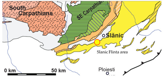
Figure 1.
The petro-gasiferous and gasiferous structures of Slanic studies (Based to student courses) Romania (Maps of Guveramental Autority).
This area forms a significant geological “depression” (a basin) that is sandwiched between two other major zones (Figure 1):
- -
- Its northern flank rests on the Flysch Zone;
- -
- Its southern flank rests on the Moesian Platform.
The creation (former) of this Diapir Folds Area involved both of these “neighbors”.
It is a classic “premontane depression” (a basin formed in front of a mountain range) sitting on a “mixed foundation” of rock from both the Flysch Zone and the Moesian Platform [11].
2. Geological Background
2.1. Analysis of the Driving Forces and Kinematics of Salt Movement
Diapirism is a geological process in which a “blob” of relatively light, “gooey” material (such as salt or high-pressure mud) pushes straight up through the heavier, more brittle rock layers above it.
The best analogy is a lava lamp, which addresses the problems related to this study:
- -
- “gooey” wax at the bottom is the salt (it is mobile and ductile);
- -
- heavier liquid it rises through is the overlying rock (it is denser);
- -
- upward movement of the wax blob is diapirism.
When this process involves salt specifically, it is called halokinesis (or salt tectonics), and kicking it off and controlling how the salt “blob” (the diapir) grows is a complex balancing act.
It depends on the “push” (the driving forces, such as buoyancy) and the physical properties (such as weight and strength) of both the salt itself and the rock layers piled on top of it [12].
Historically, scientists believed that the main reason salt moves upward (diapirism) was simple buoyancy.
This is the “lava lamp” effect, and explains these aspects:
- -
- Salt is relatively light (around 2160 kg/m3);
- -
- The sediments (like mud and sand) that pile on top of it are compacted and become much heavier (over 2500 kg/m3).
This density difference makes the light salt want to “float” upward, just like a cork in water [10].
While buoyancy is a significant factor, especially later on, modern studies show that the initial trigger is often differential loading.
The problem analysis in this paper asks and responds to the following:
- -
- What it is: Imagine the rock layers (overburden) on top of the salt are uneven—thicker in one spot and thinner in another.
- -
- How it works: This uneven weight creates a pressure difference. The salt, which can flow like thick honey, is “squeezed” away from the high-pressure area (under the thick rock) and flows toward the low-pressure area (under the thin rock). This is what kicks off the movement.
In this paper, we analyze three main “models” for how a salt diapir can grow, though in nature, most are a mix of these types [13].
2.1.1. Passive Diapirism (Downbuilding)
This is the “doughnut” model, in which the salt and sediments grow simultaneously:
- -
- The top of the salt stays at or near the seafloor.
- -
- Sediments, instead of covering the salt, pile up around it in adjacent “sinks” (called minibasins).
- -
- From the side, it looks like the salt is “sinking”, but in reality, the seafloor around it is “building up”. This is why it is called downbuilding.
- -
- This process creates specific folds and shows layers of sediment that get thicker as you move away from the salt [14].
2.1.2. Active Diapirism (Upbuilding or Forceful Intrusion)
This is the “punch” model, which happens after sediments are already in place:
- -
- A pre-existing, buried salt layer “wakes up”;
- -
- It forcefully punches its way up, piercing through the consolidated, more complex rock layers above it;
- -
- For this to happen, the salt’s pressure must be strong enough to break and lift the rock on top, causing significant bending (arching) and breaking (faulting) [15].
2.1.3. Reactive Diapirism
This model is “reacting” to large-scale tectonics and is described as follows:
- -
- The entire region is being stretched apart (extension);
- -
- This stretching causes the brittle rock on top to crack and form faults, creating zones of weakness;
- -
- The weak salt below “reacts” to this, flowing up into these cracks and thinned-out areas, often forming long salt walls [15].
The upward movement of salt creates the bends (folds) and breaks (faults) that form hydrocarbon traps [16].
However, the way the diapir grows (its “kinematic model”) is the most important factor in determining if that trap will actually hold any oil or gas.
It all comes down to timing.
The Golden Rule applied to the study of whether the trap must be built and in place before the oil and gas (hydrocarbons), in this study we ascribe to the following features:
- -
- The passive (downbuilding) scenario is an ideal setup. In this model, the traps are formed at the same time as the reservoir rocks are being deposited. The “container” is built and ready just as the nearby source rocks start “cooking” and releasing oil. This synchronous timing is perfect.
- -
- The active (upbuilding) scenario is a risky bet. In this model, the trap is formed long after the rocks were deposited and buried. This creates a race against time. For the trap to be successful, it must finish forming before the oil has migrated past that spot.
This study analyzes the possibilities for rock failure and whether if the salt punches through the rock after the oil has already moved through the area, the new structure—no matter how perfectly shaped—will be empty (barren) [17].
2.2. Analysis of the Influence of Salt Rock on Oil Maturation
Rock salt is a crystalline solid and a multiplane sedimentary rock (shale or sandstone).
It is an excellent conductor of heat, typically two to four times better than other rocks [18]:
- -
- Think of heat in the Earth’s crust like electricity; it flows from hot to cold along the path of least resistance. Because salt is so conductive, it acts as the “path of least resistance”. A salt body, therefore, acts like a “heat pipe” or a “lens,” and it effectively “sucks” heat from the sediments beneath it and channels that thermal energy straight up to its top.
- -
- This heat-focusing effect creates a distinct two-part, or “dipole”, thermal anomaly (ask and respond) and our study analysis is as follows:
- Supra-salt heating (the hot spot):
- -
- What it is: Heat is concentrated at and above the top (crest) of the salt diapir.
- -
- The result: Sediments above the salt are heated to temperatures significantly hotter than usual for their depth. It is like having a “hot plate” just below them, increasing the local temperature [19].
- Sub-salt cooling (the cold shadow):
- -
- What it is: The area beneath the salt body is “shielded” from the Earth’s natural heat flow, which has been rerouted around it.
- -
- The Result: This creates a “thermal shadow”
Sediments below the salt are insulated and remain substantially cooler than other rocks at the same depth, and this effect can be massive, with temperatures reduced by as much as 85 °C. This entire “heat pipe” effect becomes even stronger as the salt approaches the surface, where the contrast between the highly conductive salt and the porous, water-filled sediments is most excellent. This “hot top, cold bottom” effect is a master control with regard to where and when oil and gas has formed “thermal oil” (matured), and the “hot spot” above the salt dramatically speeds up the maturation of source rocks and these rocks can enter the “oil window” (the perfect cooking temperature) at much shallower depths than usual.
This can cause a very early release of hydrocarbons, which then fill the traps forming nearby [20] and the “cold shadow” below the salt dramatically slows down or even stops the cooking process, and this is a crucial preservation mechanism. Source rocks at extreme depths, which would typically be “overcooked/over-formed thermal oil” (burnt to gas or barren), are instead kept perfectly in the peak oil-generation window by the cooling, insulating effect of the salt “umbrella” above them.
These mature geological structures create a “sub-salt preservation zone” and are the reason some of the world’s largest, most recent oil discoveries are in these deep, sub-salt areas [21].
2.3. Romanian Condition of the Diapiric Geological Analysis
This paragraph describes the “stratigraphy”, or the chronological stack of rock layers, found in the Diapir Folds Area.
These layers range from the Eocene (oldest) to the Quaternary (youngest) [22].
Here is a breakdown of the layers, from oldest to youngest, based on drilling data [23]:
Eocene (Oldest):
- -
- Found only episodically in the deepest drill holes.
- -
- Rock type: Mostly “pelitic”, which means it is made of fine-grained mud and shale.
Oligoce
These layers are also dominated by mudstone/shale (pelitic), and even the sandy parts (the Kliwa facies) have a high clay content.
Sequence: drills show a stack of the following:
- -
- A lower complex of sand and mud (“psamo-pelitic”);
- -
- A horizon of pure mud (“pelitic”);
- -
- An upper complex of sand and mud;
- -
- A final horizon of transitional clays.
Thickness: This stack alone can exceed 1000 m in thickness.
Lower Miocene (Burdigalian/”Helvetian”)
This period left a sequence of the following a [23]:
- -
- brown horizon containing evaporites (salt-related deposits);
- -
- brown stony-marly horizon (marl is a mix of clay and lime);
- -
- gray sandy-marly horizon;
- -
- shale (marly) horizon.
In this area thickness is a massive sequence, measuring over 3000 m thick in some boreholes.
Badenian (Middle Miocene)
These layers are not continuous.
They were deposited patchily around the rising salt folds and are found in relatively few drills.
A sequence of geological structures is present and consists of the following [23]:
- -
- Marls and tuffs (volcanic ash) with globigerina (a microfossil);
- -
- An upper “salivary” horizon (another evaporite/salt term);
- -
- A shale horizon with radiolarians (microfossils);
- -
- A marl horizon with spirialis (microfossils).
Sarmatian (Upper-Middle Miocene)
This is another very thick sequence, divided into the following a [23]:
- -
- lower marly horizon (which is discontinuous);
- -
- main marly horizon;
- -
- calcareous sandstone horizon (a mix of lime and sand).
Thickness: The total thickness of the Sarmatian can exceed 2000 m.
Pliocene (Youngest Key Layer)
Rock Type: An alternating mix of sandy layers (“arenitic”) and mud/clay layers (“pelitic”).
- -
- Deposition: These layers were deposited “transgressively”, meaning they were laid down as the sea level rose, blanketing the older, already-folded rocks below.
- -
- Thickness: This section is also massive, exceeding 2000 m.
- -
- Crucial Feature: A specific layer called the Pontian is essential. It is made almost entirely of marl (mud/clay). It plays two key roles. Firstly, it acts as a “screen,” or seal, that traps oil and gas (hydrocarbons) from escaping. Secondly, it may also be responsible for locally generating overpressures (abnormally high fluid pressures).
2.4. Tectonics of the Diapir Zone Folds
Geologically, the area studied in this paper (located between the Slănic of Buzău Valley and the Dâmbovița Valley) is characterized by a large thrust sheet (known as a charriage), and massive slab of rock that has been pushed from north to south.
This sheet also has a transgressive character, meaning it was deposited on top of older rocks as sea levels rose, covering the pre-existing flysch deposits on the northern edge of the area (see Figure 2), and diapirism in this region (the salt structures) is categorized into several “structural alignments” based on the intensity and stage of their diapiric growth:
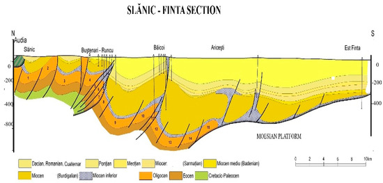
Figure 2.
Synthetic geological section (adapted to our student course).
- -
- Spilled (Extrusive) Diapirism: The most intense form, where the salt has completely broken through all overlying rock and “spilled” onto the surface.
- -
- Exaggerated Diapirism: Very mature, large-scale diapirs that have forcefully pierced and deformed the rock layers above them.
- -
- Attenuated Diapirism: A less intense or “thinned out” form, where the diapir’s growth has slowed, or the salt source is being depleted.
- -
- Early Diapirism (Cryptodiapir): The earliest stage. This refers to “hidden” or “incipient” salt structures (such as salt pillows) that have begun to rise but have not yet broken through the overlying rock layers.
2.5. Formation Conditions of Hydrocarbon Reservoirs
To describe the complete petroleum system of the Diapir Folds, we analyze the source rocks (where oil forms), the reservoir rocks (where it is stored), the seal rocks (what traps it), and the role of the salt in creating the hydrocarbon reservoirs.
- 1.
- Source Rocks (The “Mother Rocks”),
The “mother rocks”, or source rocks, that generated the hydrocarbons are found in numerous geological layers and typically dark, organic-rich shales:
Oligocene: Menilitic and disodilic shales.
Podul Morii (Oligocene): Clayey shales.
Aquitanian (Miocene): Bituminous (oil-rich) shales.
Helvetian (Miocene): Bituminous calcareous shales.
Tortonian (Miocene): Radiolarian shales.
Buglovian and Sarmatian (Miocene): Bituminous calcareous shales [24].
Even the younger Pliocene mudrocks (Meotian, Pontian, Dacian, and Levantine) are considered source rocks in some structures.
- 2.
- Reservoir Rocks (The “Storage Tanks”)
The reservoir rocks, which have the porosity and permeability to hold the oil and gas, are as follows:
- -
- Sands;
- -
- Marly sands;
- -
- Sandstones.
In some specific locations, like the Sarmatian-age Boldesti structure, microconglomerates also act as reservoir rocks.
- 3.
- Seal Rocks (The “Lid”)
The “protective” or seal rocks (cap rocks) that prevent the hydrocarbons from escaping are the pelitic (shale and clay) layers.
In this system, the same rocks often played two roles; they first served as the source rock, and after expelling their hydrocarbons, their impermeability allowed them to act as the seal rock that trapped those same hydrocarbons.
- 4.
- The Role of Salt: A Mechanical Architect, Not a Pathway
The connection between the salt diapirs and the hydrocarbon reservoirs is purely mechanical.
The authors argue against the idea of vertical migration. Since salt is impermeable, there is no evidence to suggest that hydrocarbons migrated vertically along the salt’s walls from older formations (like the Oligocene) into newer ones (like the Miocene or Eocene).
Instead, the hydrocarbons likely formed within or near their reservoir layers and migrated laterally and the salt’s critical role was to physically build the traps.
The upward movement of the salt (diapirism) is what bent, folded, and faulted the surrounding rock layers, creating the structures where oil and gas could accumulate.
- 5.
- Trap Types (The Final Structures)
The rising salt created several specific types of traps:
- -
- In the Pliocene: Traps are “vaulted” (arched domes), “compartmentalized” (broken into blocks by faults), or “tectonically shielded” (sealed against a fault).
- -
- In the Oligocene, Helvetian, Buglovian, and Sarmatian: Traps are typically “stratiform” (following a specific rock layer) and “stratigraphically screened” (where the reservoir rock pinches out or changes into a non-porous rock).
In conclusion, in this chapter, geological and geophysical studies (especially drilling results) have confirmed that this area is defined by a series of linear diapiric structures. These structures run parallel to the Carpathian mountain chain and are directly linked to the region’s major oil and gas fields [25].
2.6. Productive Structures
The distribution of oil fields in the Carpathians is not random and it is the direct result of an interaction between two key factors:
- -
- Regional tectonic squeezing (compression);
- -
- The original shape of the pre-existing salt basin.
The “exaggerated diapirism alignment”, which defines the entire Diapiric Fold Zone, is simply the surface expression of deep-seated thrust faults.
These faults are “greased” or “lubricated” by the deep salt layer, allowing them to move, and an understanding of this provides a powerful predictive tool for exploration.
To find the most promising oil-bearing structures (folds) in the belt, exploration teams should first map the geometry of the original salt basin buried deep below [26].
Through analysis and using data from more representative wells it is possible to identify an exaggerated diapirism alignment, mentioned previously; the structures in this area are grouped by the intensity of the salt’s movement and their structural alignment (see Figure 2).
In this alignment, the salt diapirs (which are located just below the youngest Quaternary deposits) form asymmetric anticlines (uneven arches) and these structures are faulted, with the northern flank consistently pushed up and over the southern flank [27].
Major production of oil is present in this alignemnt.
3. Analysis of the Petroligene Potential
In this chapter, an analysis of complex studies of the influences of diapirism rocks based on thermal maturation is conducted to estimate the potential of oil.
We devised a new equation for the TTI (Time–Temperature Index) method and created an AI model.
This method, the TTI (Time–Temperature Index), was first developed by Lopatin [27] and later refined by Waples [28], and this method is based on two simple things:
- Burial History (time) refers to how long a source rock has been buried;
- Temperature is a good factor for analyzing exposure to thermal maturation over time.
The core scientific principle is the Arrhenius relation, which states that for every 10 °C (18 °F) increase in temperature, the chemical reaction rate (the “thermal maturation” speed) doubles [28].
By adding up the “time + temperature” exposure, the TTI calculates a final “thermal maturation” score for the rock, and a TTI score is incredibly useful for determining the depths at which you are likely to find resources (oil, wet gas, or dry gas), whether the source rocks have entered the “generative window”, and the timing of hydrocarbon generation (i.e., when the oil reached “thermal maturation”).
Geologists know a rock is in the “oil window and/or mature oil formation” phase when it meets these specific criteria [29]:
- -
- Temperature Range: 60 °C to 150 °C (140 °F to 300 °F).
- -
- Vitrinite Reflectance (%R0): 0.6% to 1.3% (a measure of how “shiny” coal fragments in the rock are).
- -
- Tmax (from rock-eval pyrolysis): 435 °C to 455 °C (a lab-based “baking” test).
If a rock is below this window, it is immature (not cooked enough).
If it is above this window, it is overmature and has cooked past the oil stage, producing primarily gas, and the oil window is the “Goldilocks” zone that the TTI method helps to identify.
A critical stage in a source rock’s life is the point at which it reaches the perfect temperature and maturity for kerogen (the raw organic matter) to break down (a process called catagenesis) and generate liquid oil [29].
3.1. Formation Conditions of the Oil Window
The maturation stages are related to the specific temperature and maturity ranges where source rock generates liquid oil (Table 1).

Table 1.
Rock’s “cooked-ness” (maturity), sorted into distinct stages [30].
There are also four different kerogen types that mature differently and affect oil window characteristics [31]:
- -
- Type I (Algal/Lakes): The best for oil. It can enter the oil window early (around 0.5% Ro) and yields high volumes of oil.
- -
- Type II (Planktonic/Marine): The most common contributor to global oil. It generates oil over a wide maturity range.
- -
- Type III (Woody/Terrestrial): Poor for oil. This “gassy” kerogen usually skips the oil phase and generates natural gas at higher maturities (>1.0% R0).
3.2. Technical Details of Geological Analysis of Oil Window
In our laboratory we use several lab tools to determine if a rock is in the oil window:
- Vitrinite reflectance (%R0) is an industry standard and consist of analysis and optical measurement of how “shiny” (reflective) coaly particles (vitrinite) in the rock are. The shinier the particle, the more “cooked” it is.
- Rock-eval pyrolysis is a lab test that “bakes” a rock sample to see what hydrocarbons it can still produce.
- Tmax is the temperature at which the rock releases the most hydrocarbons, indicating its maturity.
- S2 peak analysis identifies how much hydrocarbon potential is left in the rock.
- Hydrogen index (HI) measures the hydrogen-richness of the kerogen. The HI decreases as the rock matures and generates oil.
- Biomarker ratios relate to specific “molecular fossils” (like steranes and hopanes) that change their chemical structure in predictable ways as the temperature increases.
Determining what controls the “thermal maturation” process (geological controls), requires an analysis of the burial history (as deeper and longer burial means more time at higher temperatures, which speeds up maturation); geothermal gradient (this is the “oven’s temperature setting” for the basin, with a high geothermal gradient (a “hot” basin) “cooking” rocks faster and at much shallower depths); and tectonic activity (uplift and erosion can cool the rock, slowing or completely stopping the maturation process).
In our analysis, the depth of the oil window depends entirely on the geothermal gradient (Figure 3). These are divided into a cool basin (low gradient, e.g., 25 °C/km), where the oil window may be very deep (from 2.5 to 5 km), and a hot basin (high gradient, e.g., 40 °C/km), where the oil window will be much shallower (from 1.5 to 3.5 km).
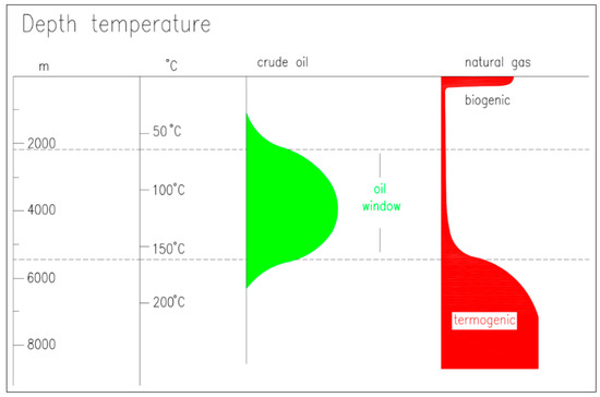
Figure 3.
Oil window formation.
For example, in a “hot” area like the Gulf of Mexico, the oil window can be as shallow as 2 km.
In “cool”, stable basins, it may not start until over 4 km deep.
To calculate this, the Waples (TTI) method is used and this requires creating a burial history chart for each rock layer (Figure 4), where Curve A (Figure 4) shows a rock that was buried slowly at first, then experienced faster, steady burial (subsidence) and Curve B (Figure 4) shows a more complex history.
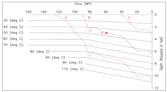
Figure 4.
Burying model for the A, B, and C horizons (adapted from Waples, 1980 [29]).
This layer was buried, then experienced an uplift phase (moving it closer to the surface and cooling it), and finally returned to a normal burial (subsidence) regime (curve C-Figure 4).
Waples also proposed a series of values for the TTI calculation and the r parameter derived from Waple’s theory [29] (based on Figure 4).
In Table 2, we present the calculation TTI values for our geological model.
Table 2.
Calculation of present TTI values geological models.
Depending on the depth of burial, the sediments were subjected to temperatures consistent with the regional geothermal gradient, and the calculation relationship is formed to the following relationships [29]:
where
- MA—millions of years;
- t—time;
- r—temperature depends on coefficient.
Using this calculation relationship, the various values of the parameter r can be determined depending on the temperature range. Based on the work of Waple, we propose a new equation to calculated the temperature factors function in relation to different temperature intervals [29].
In our analysis, based on research with 1000 data points, we proposed a new equation based on the following regressional forms [30]:
For the horizon A:
For the horizon B:
For the horizon C:
The three equations are multiple regression models for the three horizons.
In this article, we have created an AI model (Random Forest) with the following characteristics (Figure 5):
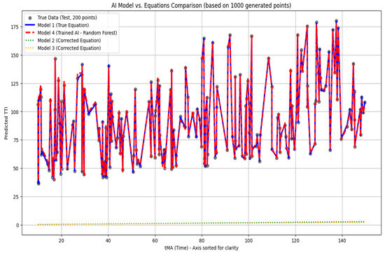
Figure 5.
Neuronal AI models of actual TTT values and predicted TTT values (200 training samples and 800 testing samples).
- -
- The model correctly learned that ‘n’ is the most important variable (80.4%) for predicting TTI, followed by ‘tMA’ (19.1%);
- -
- This fits perfectly with Equation (2) (the truth), where n has the largest coefficient (10.16 and tMA has the second largest (0.22);
- -
- Generated 1000 data points;
- -
- Trained model 4 (AI) with 800 data points;
- -
- Model 4 trained and tested on 200 data points.
To perform the interconversion of the Thermal Alteration Index (TAI) and vitrinite reflectance values (R0), Waples proposed different values for the Interconversion of Thermal Alteration Index (TAI) and vitrinite reflectance values (R0) for different vitrinite reflectance values depending on TAI [30,31].
To resolve Equation (1) an interconversion of Thermal Alteration Index (TAI) and vitrinite reflectance values (R0) is required.
The equation based on the Waples value to Interconversion of Thermal Alteration Index (TAI) and vitrinite reflectance values (R0) for different vitrinite reflectance values depending on TAI (Figure 6) is as follows [31,32,33]:
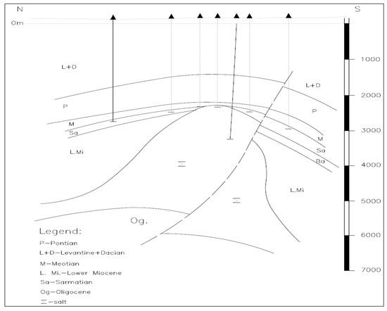
Figure 6.
Representative geological section (well 5501)—Moreni structure.
These equations are designed to analyze 1000 data points related to oil exploration.
4. Diapir Folds Area from Romanian Case Studies
Here we start from Lopatin’s time threshold values—the maturity temperature index (TTI) and the vitrinite reflectance (R0).
We proposed a numerical equation to determine the values that could be considered as references as well as the thresholds after which the generation of hydrocarbons (oil and gas) takes place; the sediment burial curves were simulated and drawn for two wells in the Diapir Folds Area of Romania.
This equation (experimental analysis) analyses the TTI function in relation to the vitrinite reflectance (R0):
where TTI is 5 for onset of oil generation, 75 for peak oil generation, 160 for the end of oil generation, 500 for the upper TTI limit for occurrence of oil with API gravity < 40°, 1000 for the upper TTI limit for occurrence of oil with API gravity < 50°, 1500 for the upper TTI limit for the occurrence of wet gas, 65,000 for the last known occurrence of dry gas, and 972,000 for liquid sulfur in Lone Star Baden 1 (below dry gas limit) [29].
TTI = 0.4474 ln(R0) − 0.8732
R0 = 8.7839e2.1402 TTI
In this sense, the following were used:
- -
- Depth data;
- -
- Time (MA), determining the age of the deposited formations;
- -
- The temperature.
Then, each of the following were calculated:
- -
- The TTI index;
- -
- The “r” parameter, the function of which reveals the TTI index;
- -
- The amount of TTI data as a function of vitrinite reflectance (R0) and entry into the oil window.
For each well analyzed, a representative geological section was created, indicating the geological age of the formations, the depth, and the presence of salt.
Also, each well is represented (on the right side) in the simulations by a representative lithological column.
Both wells were in the exaggerated diapirism (previously presented) in the Diapir Folds Area.
The Moreni structure (Figure 6) is presented in the form of an asymmetric anticline with the northern flank higher by about 1000 m and straddling the southern one. Hydrocarbon deposits are concentrated in the Levantine, Dacian, Helvetian, Meotian, and Oligocene periods.
Well 5501 Piscuri
From (Figure 7), the ages of the geological formations (millions of years) were read:
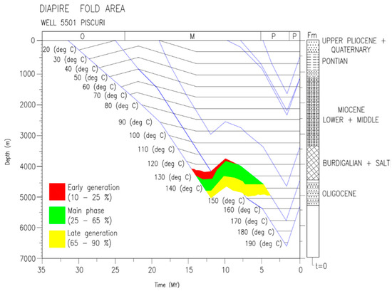
Figure 7.
Simulation of sediment burial curves—well 5501 Piscuri.
- -
- Up to 70 °C—Oligocene (23–35 MA);
- -
- Between 70 and 150 °C—Miocene (5–24 MA);
- -
- After 150 °C—Pontian (0–5 MA).
According to (Table 3), the vitrinite reflectance (R0) for well 5501 Piscouri is as follows (Figure 8):
Table 3.
Time and temperature data structuring, TTI.
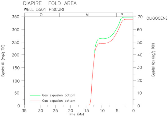
Figure 8.
Decompression simulation—well 5501 Piscuri.
- -
- R0 = 0.65 for TTI—15—the onset of oil generation (sum of points 1–12)—temperature range 20–30–130–140 °C;
- -
- R0 = 1 for TTI—75—oil generation peak (between point 12 and point 13)—after temperature interval 140–150 °C (6 Ma—late generation).
The determination of the depth at which the formation is found (decompaction simulation) is shown in Figure 9.
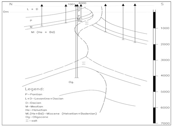
Figure 9.
Representative geological section (well 6000)—Moreni structure.
The calculation of the time (M.a.) the “r” index, and the TTI, respectively, is shown in Table 2.
Well 6000 Bis Moreni
The ages of the geological formations (millions of years) were read from (Figure 10):
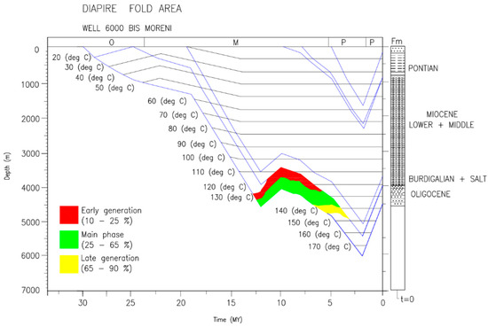
Figure 10.
Simulation of sediment burial curves—well 6000 Bis Moreni.
- -
- Up to 50°—Oligocene (23–29 M.A.);
- -
- Between 80° and 140°—Miocene (5.2–23 M.A.);
- -
- After 150°—Pontian (0–5.2 M.A.).
The calculation of the time (M.a.) the “r” index, and the TTI, respectively, is shown in Table 4.
Table 4.
Time and temperature data structuring, TTI, well 6000, Moreni structure.
According to Equations (7) and (8), the vitrinite reflectance (R0) for the 6000 Bis Moreni is as follows (Figure 9):
- -
- R0 = 0.65 for TTI—15—the onset of oil generation (sum of points 1–12)—temperature range 20–30—130–140 °C;
- -
- R0 = 1 for TTI—75—oil generation peak (between point 12 and point 13)—after temperature interval 140–150 °C (6 MA—late generation).
- -
- The determination of the depth at which the formation is found (decompaction simulation) is shown in (Figure 10 and Figure 11).
 Figure 11. Decompression simulation—well 6000 Bis Moreni.
5. Conclusions
Salt tectonics plays two primary, powerful roles in forming petroleum provinces. It simultaneously controls the physical structure of the basin and dictates its thermal history.
- Tectonic Control (The “Master Detachment”)
In compressional settings like the Eastern Carpathians, thick salt layers act as fundamental zones of mechanical weakness.
- -
- When the Alpine Orogeny applied regional “squeezing” (compression), the stress was focused along the weak Miocene salt horizon.
- -
- This salt layer acted as a “master detachment surface”—a greasy layer allowing the rock units above it to slide and fold.
- -
- Thrust faults started within this salt layer and propagated upwards, creating the characteristic salt-cored folds and nappes seen today.
- -
- This means the salt actively controlled the structural style of the entire fold-and-thrust belt; it was not just a passive player.
- 2.
- Thermal Control (The “Two-Play System”)
Salt’s thermal properties are completely different from those of sedimentary rock. This fundamentally decouples the petroleum systems above and below the salt.
- -
- Supra-Salt (Above): This domain has its own thermal regime, maturation history, and exploration play.
- -
- Sub-Salt (Below): This domain operates under a completely different thermal regime, creating a second, separate play.
This allows two superimposed, but distinct, petroleum systems to exist in the same geographic area. The salt-driven process (halokinesis) is highly efficient, as it creates all the necessary elements: a rich variety of traps, complex migration pathways, and a near-perfect seal.
- 3.
- The Carpathian Case Study
This theory is perfectly demonstrated in the Eastern Carpathians.
- -
- The vast majority of oil fields are clustered within the Diapiric Fold Zone (e.g., Moinesti area);
- -
- Prolific fields like Runcu-Buștenari and Colibași define the regional play type;
- -
- The play consists of the Kliwa Sandstone (the primary reservoir), which is trapped in complex salt-cored anticlinal structures [26];
- -
- The association with sand intrusions also highlights a dynamic link between salt movement and the creation of enhanced reservoirs.
- 4.
- Present Study: Modeling the Oil Window
To quantify this, the present study modeled the burial and thermal history for two representative wells in the Diapir Folds Area.
- -
- Method: The study used the classic Waples (TTI) algorithm. Burial curves were built using specialized software that also simulated the decompaction of sediments over time.
- -
- Results: The modeling defined the key maturation benchmarks for oil generation in these wells:
Onset of Oil Generation: Occurs between 130 and 150 °C, corresponding to a TTI of 15 and a vitrinite reflectance.
- -
- Peak Oil Generation: Reached at a TTI of 75 (R0 = 1.0%).
- -
- End of Oil Generation: The oil window closes at a TTI value of 160.
Author Contributions
Conceptualization, C.V.V. and T.-V.C.; methodology, C.V.V.; software, T.-V.C.; validation, C.V.V. and T.-V.C.; formal analysis, H.A.; investigation, S.A.; resources, T.-V.C.; data curation, C.V.V.; writing—original draft preparation, C.V.V.; writing—review and editing, T.-V.C.; visualization, T.-V.C.; supervision, T.-V.C.; project administration, T.-V.C.; funding acquisition, T.-V.C. All authors have read and agreed to the published version of the manuscript.
Funding
This research received no external funding.
Institutional Review Board Statement
The study was conducted in accordance with the Declaration of Helsinki and approved by the Institutional Review Board and Ethics Committee of Petroleum-Gas University Declaration.
Informed Consent Statement
Informed consent was obtained from all subjects involved in the study.
Data Availability Statement
The original contributions presented in this study are included in the article. Further inquiries can be directed to the corresponding author.
Acknowledgments
During the preparation of this manuscript, the authors used AI software. The authors have reviewed and edited the output and take full responsibility for the content of this publication.
Conflicts of Interest
The authors declare no conflicts of interest.
Abbreviations
The following abbreviations are used in this manuscript:
| TTI | Time–Temperature Index |
| TAI | Thermal Alteration Index |
| Ro | Vitrinite Reflectance Values |
References
- Jackson, M.P.A.; Hudec, M.R. Salt Tectonics: Principles and Practice; Cambridge University Press: Cambridge, UK, 2017; pp. 464–494. [Google Scholar]
- Alsop, G.I.; Carreras, J. Structural evolution of sheath folds: A case study from Cap de Creus. J. Struct. Geol. 2007, 29, 1915–1930. [Google Scholar] [CrossRef]
- Alsop, G.I.; Holdsworth, R.E. The geometry and kinematics of flow perturbation folds. Tectonophysics 2002, 350, 99–125. [Google Scholar] [CrossRef]
- Soto, J.I.; Tim Dooley, P.; Hudec, M.R.; Peel, F.J.; Apps, G.M. Shortening a mixed salt and mobile shale system: A case study from East Breaks, northwest Gulf of Mexico. Interpretation 2024, 12, SF77–SF103. [Google Scholar] [CrossRef]
- Ziegler, P.A. Geodynamics of rifting and implications for hydrocarbon habitat. Tectonophysics 1992, 215, 221–253. [Google Scholar] [CrossRef]
- Rossello, E.A.; Osorio, J.A.; López-Isaza, S. El diapirismo argilocinético del Margen Caribeño Colombiano: Una revisión de sus condicionantes sedimentarios aplicados a la exploración de hidrocarburos. Boletín Geol. 2022, 44, 15–48. [Google Scholar] [CrossRef]
- Claypool, G.E.; Kaplan, I.R. The Origin and Distribution of Methane in Marine Sediments. In Natural Gases in Marine Sediments; Marine Science; Kaplan, I.R., Ed.; Springer: Boston, MA, USA, 1974; Volume 3. [Google Scholar] [CrossRef]
- Arthur, M.A.; von Rad, U.; Cornfold, C.; Mccoy, F.; Sarnthein, M. Evolution and sedimentary history of the Cape Bojador continental margin, Northwestern Africa. Init. Rep. Deep Sea Drill. Proj. 1979, 47, 773–816. [Google Scholar]
- Paull, C.K.; Dillon, W.P. Erosional origin of the Blake Escarpment: An alternative hypothesis. Geology 1980, 8, 538–542. [Google Scholar] [CrossRef]
- Grant, A.C.; McAlpine, K.D.; Wade, J.A. Offshore Geology and Petroleum Potential of Eastern Canada. Energy Explor. Exploit. 1986, 4, 5–52. [Google Scholar] [CrossRef]
- Klose, G.W.; Malterre, E.; McMillan, N.J.; Zinkan, C.G. Petroleum exploration offshore southern Baffin Island, northern Labrador Sea, Canada. In Arctic Geology and Geophysics; Embry, A.F., Balkwill, H.R., Eds.; Canadian Society of Petroleum Geologists Memoir 8; Datapages, Inc.: Tulsa, Oklahoma, 1982; pp. 233–244. [Google Scholar]
- Kristoffersen, Y. Seafloor spreading and the early opening of the north Atlantic. Earth Planet. Sci. Lett. 1978, 38, 273–290. [Google Scholar] [CrossRef]
- Hemin, K.; Christopher, J.T.; Bjørn, O.T. Salt diapirs of the southwest Nordkapp Basin: Analogue modelling. Tectonophysics 1993, 228, 167–187. [Google Scholar] [CrossRef]
- Lasabuda, A.P.E.; Johansen, N.S.; Laberg, J.S.; Faleide, J.I.; Senger, K.; Rydningen, T.A.; Patton, H.; Knutsen, S.-M.; Hanssen, A. Cenozoic uplift and erosion of the Norwegian Barents Shelf—A review. Earth-Sci. Rev. 2021, 217, 103609. [Google Scholar] [CrossRef]
- Jackson, M.; Vendeville, B. Regional extension as a geologic trigger for diapirism. Geol. Soc. Am. Bull. 1994, 106, 57–73. [Google Scholar] [CrossRef]
- Jackson, M.; Vendeville, B.; Schultz-Ela, D. Structural Dynamics of Salt Systems. Annu. Rev. Earth Planet. Sci. 2003, 22, 93–117. [Google Scholar] [CrossRef]
- Engelkemeir, R.; Khan, S. Lidar mapping of faults in Houston, Texas, USA. Geosphere 2008, 4, 170–182. [Google Scholar] [CrossRef]
- Ahoure, N.; Egoran, B.; Kouadio, G.; Sehi, Z.; Oura, E.; Digbehi, Z. Geochemical Analysis of Albian-Maastrichtian Formations in the Offshore Basin of the Abidjan Margin: Rock-Eval Pyrolysis Study. Open J. Geol. 2024, 14, 805–822. [Google Scholar] [CrossRef]
- Tyson, R.V. (Ed.) Abundance of Organic Matter in Sediments: TOC, Hydrodynamic Equivalence, Dilution and Flux Effects. In Sedimentary Organic Matter; Springer: Dordrecht, The Netherlands, 1995; pp. 81–118. [Google Scholar] [CrossRef]
- Espitalie, J.; Deroo, G.; Marquis, F. La pyrolyse Rock-Eval et ses applications. Deuxième partie. Rev. l’institut Français Pétrole 1985, 40, 755–784. [Google Scholar] [CrossRef]
- Espitalié, J.; Laporte, J.L.; Madec, M.; Marquis, F.; Leplat, P.; Paulet, J.; Boutefeu, A. Méthode rapide de caractérisation des roches mètres, de leur potentiel pétrolier et de leur degré d’évolution. Rev. l’Institut Français Pétrole 1977, 32, 23–42. [Google Scholar] [CrossRef]
- Peters, K.E. Guidelines for Evaluating Petroleum Source Rock Using Programmed Pyrolysis. AAPG Bull. 1986, 70, 318–329. [Google Scholar] [CrossRef]
- Kumar, N.; Embley, R.W. Evolution and Origin of Ceará Rise: An Aseismic Rise in the Western Equatorial Atlantic. Geol. Soc. Am. Bull. 1977, 88, 683–699. [Google Scholar] [CrossRef]
- Rddad, L.; Jemmali, N.; Jaballah, S. The Role of Organic Matter and Hydrocarbons in the Genesis of the Pb-Zn-Fe (Ba-Sr) Ore Deposits in the Diapirs Zone, Northern Tunisia. Minerals 2024, 14, 932. [Google Scholar] [CrossRef]
- Cedeño, A.; Rojo, L.A.; Cardozo, N.; Centeno, L.; Escalona, A. The Impact of Salt Tectonics on the Thermal Evolution and the Petroleum System of Confined Rift Basins: Insights from Basin Modeling of the Nordkapp Basin, Norwegian Barents Sea. Geosciences 2019, 9, 316. [Google Scholar] [CrossRef]
- Batistatu, M.V. Structural Geology; Publishing House of the Oil-Gas University of Ploiesti: Ploiești, Romania, 2020. [Google Scholar]
- Beca, C.; Prodan, D. Oil and Gas Structures in Romania; Oil and Gas Institute: Ploiești, Romania, 1981. [Google Scholar]
- Mutihac, V. Geology of Romania in the Central-Eastern-European Geostructural Context; Didactic and Pedagogical Publishing House: Bucharest, Romania, 2010. [Google Scholar]
- Waples, W.D. Time and Temperature in Petroleum Formation: Application of Lopatin’s Method to Petroleum Exploration. Am. Pet. Geol. Bull. 1980, 64, 916–926. [Google Scholar]
- Huang, Y.C. Thermal History Model of the Williston Basin. Master’s Thesis, University of North Dakota, Grand Forks, ND, USA, 1988; p. 143. Available online: https://commons.und.edu/theses/143 (accessed on 10 September 2025).
- Sarwar, G.; Friedman, G.M. Research methods. In Post-Devonian Sediment Cover over New York State; Sarwar, G., Friedman, G.M., Eds.; Lecture Notes in Earth Sciences; Springer: Berlin/Heidelberg, Germany, 2005; Volume 58, pp. 29–51. ISBN 978-3-540-49271-9. [Google Scholar] [CrossRef]
- Doukeh, R.; Ghețiu, I.V.; Chiș, T.V.; Stoica, D.B.; Brănoiu, G.; Ramadan, I.N.; Gavrilă, Ș.A.; Petrescu, M.G.; Harkouss, R. Hydrogen–Rock Interactions in Carbonate and Siliceous Reservoirs: A Petrophysical Perspective. Appl. Sci. 2025, 15, 7957. [Google Scholar] [CrossRef]
- Marandi, M.; Jahani, D.; Uromeihy, A.; Reihan, M. Analysis of Structure and Textures of Anhydrite Mineral in Gachsaran Formation in Gotvand Area, Iran. Open J. Geol. 2017, 7, 1478–1493. [Google Scholar] [CrossRef]


Disclaimer/Publisher’s Note: The statements, opinions and data contained in all publications are solely those of the individual author(s) and contributor(s) and not of MDPI and/or the editor(s). MDPI and/or the editor(s) disclaim responsibility for any injury to people or property resulting from any ideas, methods, instructions or products referred to in the content. |
© 2025 by the authors. Licensee MDPI, Basel, Switzerland. This article is an open access article distributed under the terms and conditions of the Creative Commons Attribution (CC BY) license (https://creativecommons.org/licenses/by/4.0/).