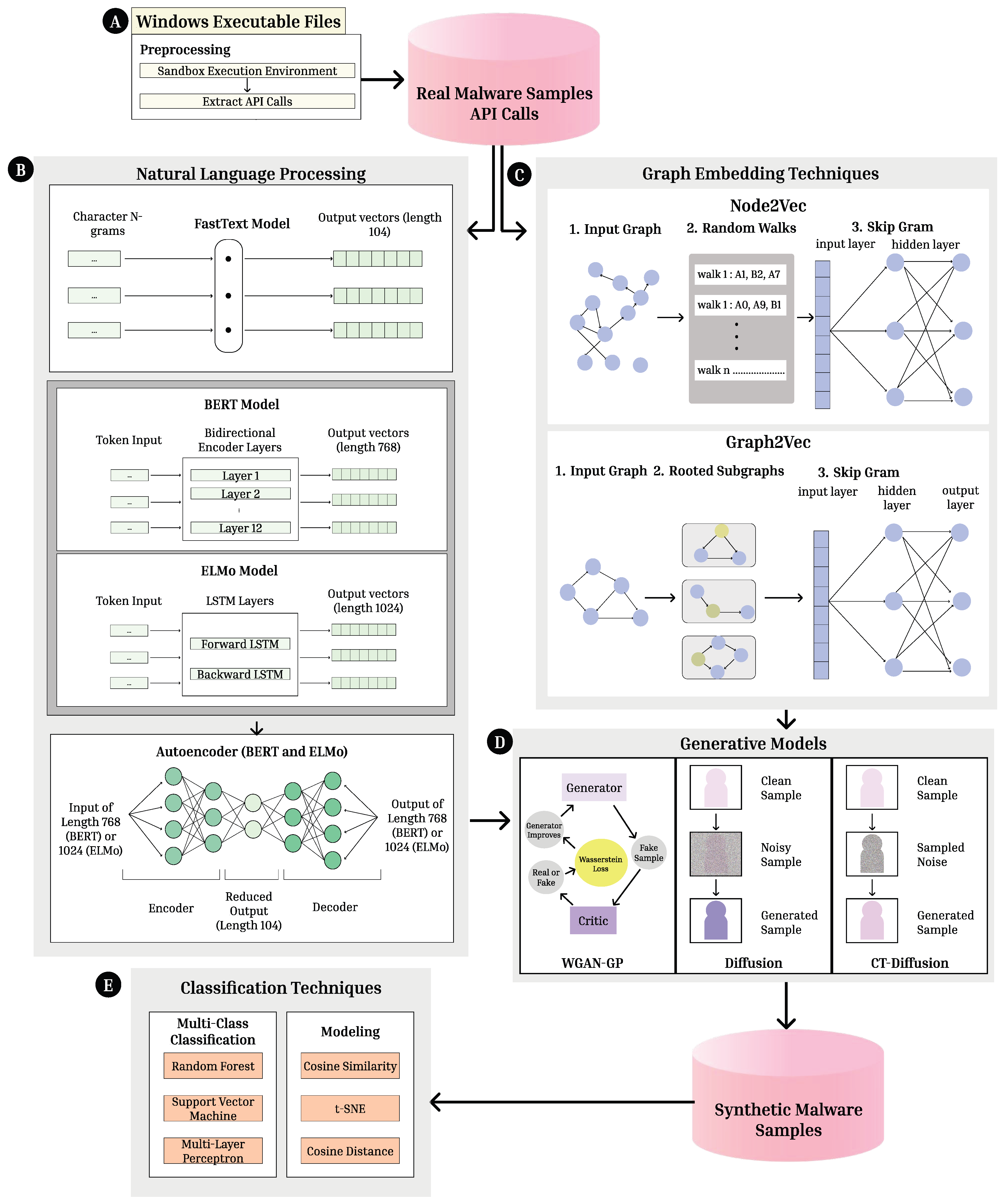
Figure 1.
System Architecture. This paper creates a system composed of five primary parts: (A) Extracting malware API calls from 7 malware families by dynamically executing Windows malware executables, (B) Natural Language Processing through 3 NLP models and dimension reduction techniques to generate vector embeddings, (C) Graph-based processing through 2 graph embedding methods to generate vector embeddings, (D) Processing word and graph embeddings through 3 Generative AI Models with an end goal of synthetic malware sample generation. (E) The use of six evaluation metrics, both multi-class classification and modeling techniques, to evaluate the generated embeddings.
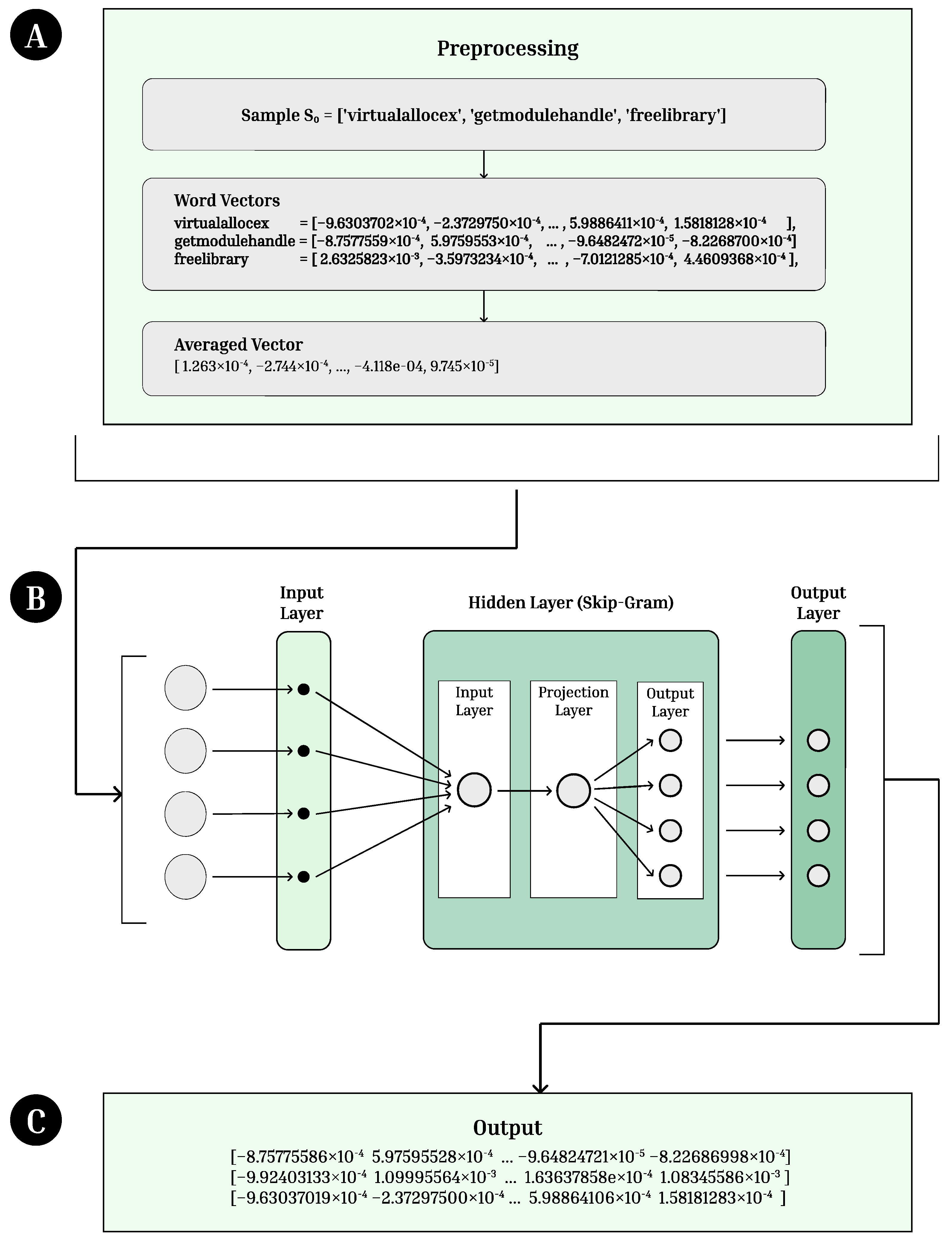
Figure 2.
FastText Architecture. (A) API call embeddings are preprocessed and turned into word vectors. (B) The vectors are passed into the FastText model. After the input layer, they are processed through a hidden layer using Skip-Gram followed by an output layer. (C) Vectors of length 104 are outputted from the model.
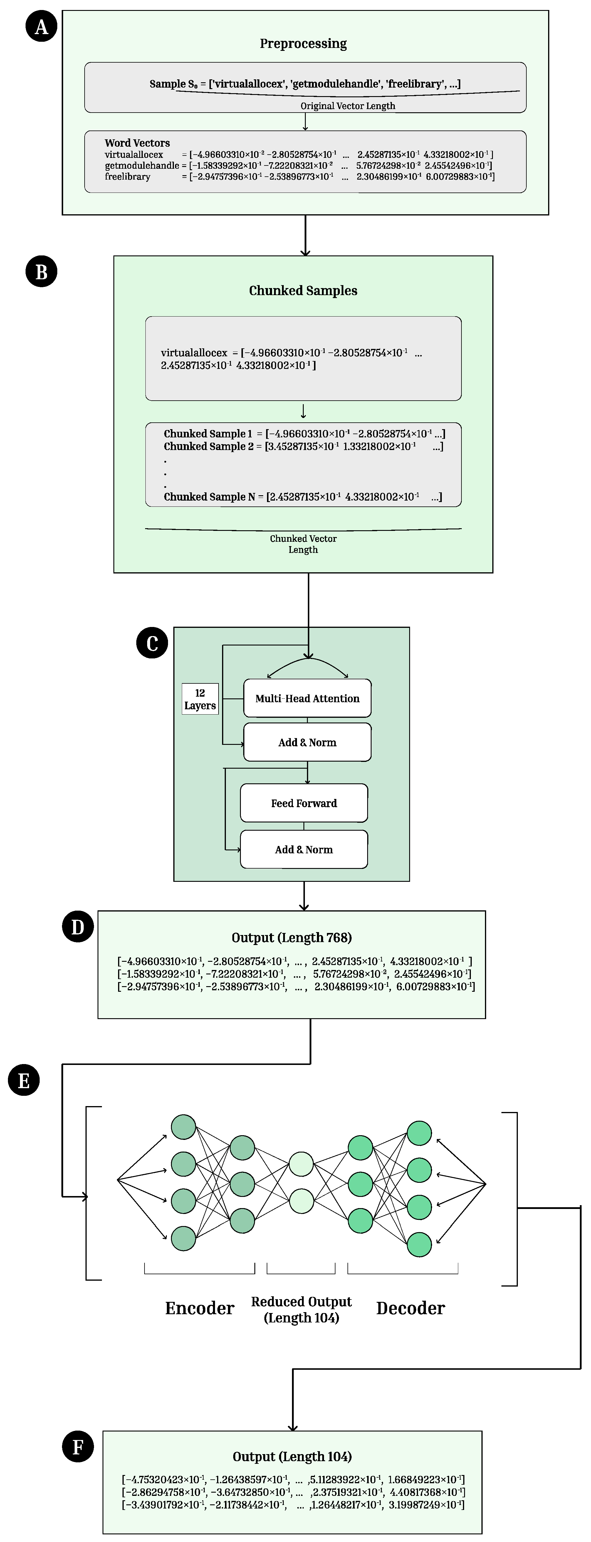
Figure 3.
BERT Architecture (A) API call embeddings are preprocessed and turned into word vectors. (B) The vectors are chunked into chunks of length 512 due to limits on the length of vector that can be passed into the BERT model. (C) The vectors are passed into the BERT model, composed of attention layers, normalization layers, and feed forward layers. (D) Vectors of length 768 are outputted from the model. (E) The vectors are processed using an autoencoder to reduce the dimension of the output. (F) Final vectors of length 104 are outputted from the autoencoder.
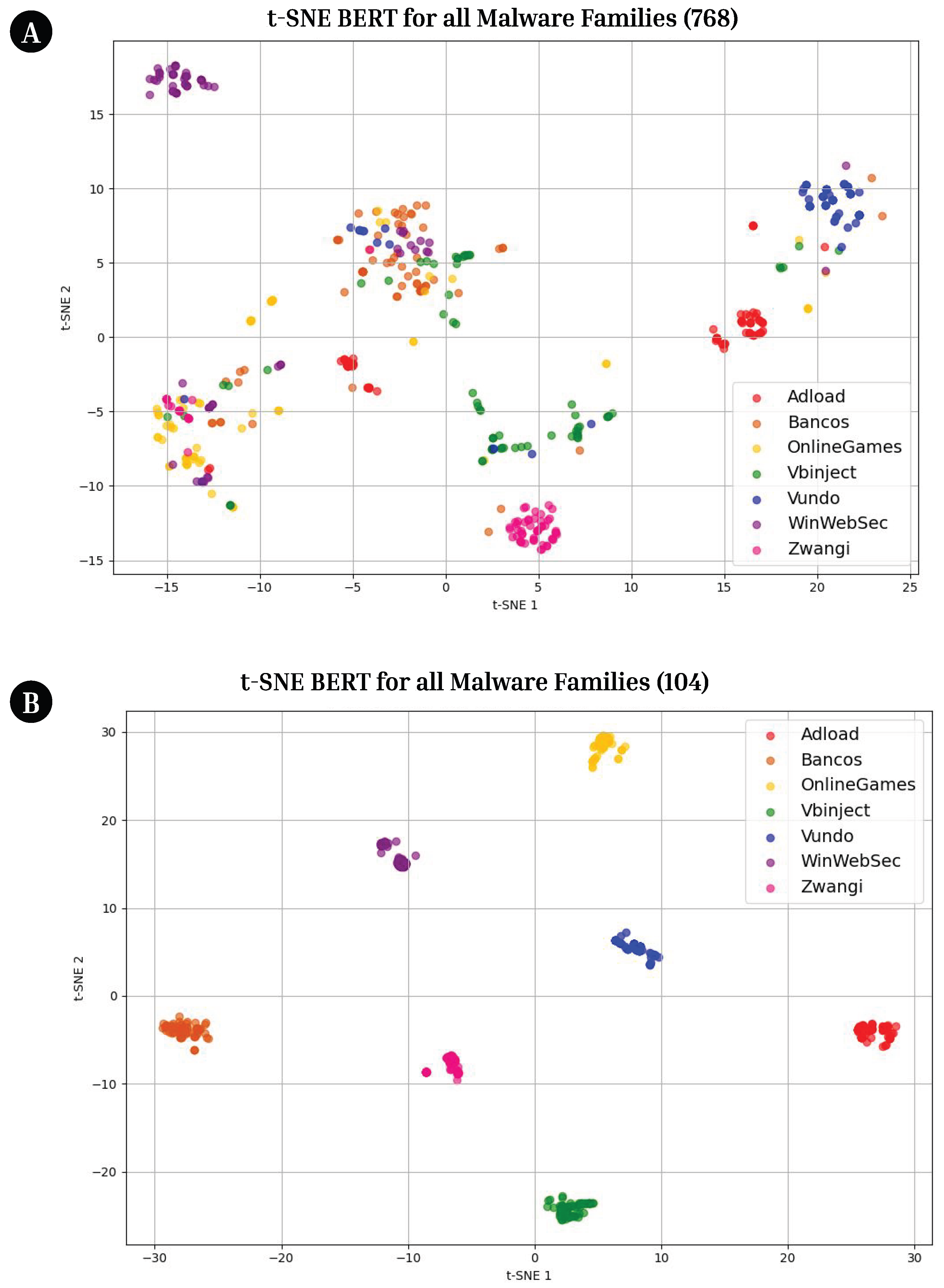
Figure 4.
tSNE Plot of BERT Embeddings with Varying Vector Length. (A) tSNE plot with BERT embeddings of length 768. The clustering is minimal, indicating that they are not distinct by family. (B) tSNE plot with BERT embeddings of length 104. Distinct clusters are formed, indicating higher-quality and improved representation of the API call data.
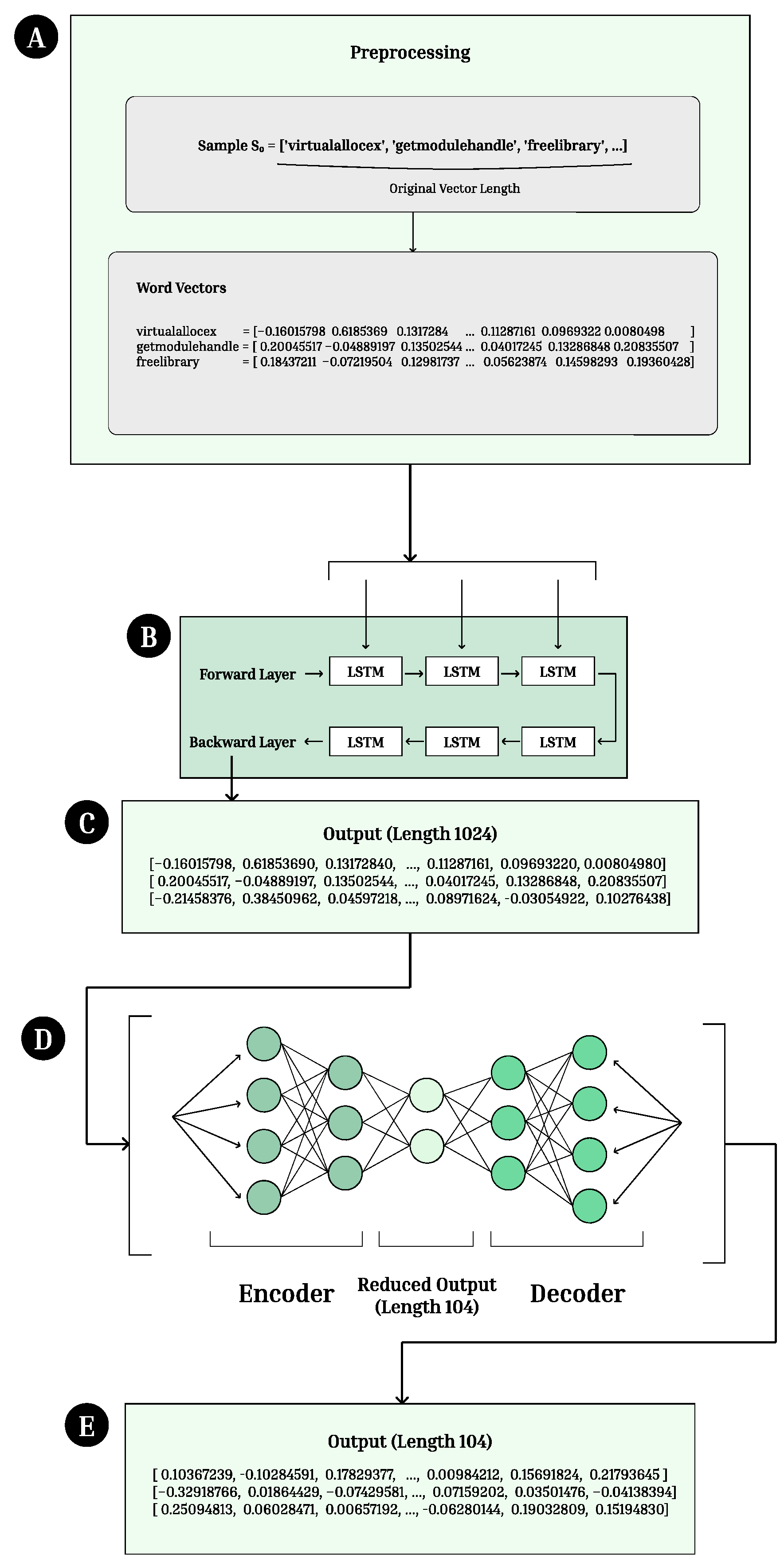
Figure 5.
ELMo Architecture. (A) API call embeddings are preprocessed and turned into word vectors. (B) The vectors are passed into the ELMo model, composed of forward and backward Long Short Term Memory (LSTM) layers. (C) Vectors of length 1024 are outputted from the model. (D) The vectors are processed using an autoencoder to reduce the dimension of the output. (E) Final vectors of length 104 are outputted from the autoencoder.
Figure 6.
Node2Vec Embedding Procedure. (1) the disconnected family wide graph structure of a node2vec embedding (2) the various random walks possible from point A, and the skip gram model vectorization (3) the generated Skip Gram embeddings.
Figure 6.
Node2Vec Embedding Procedure. (1) the disconnected family wide graph structure of a node2vec embedding (2) the various random walks possible from point A, and the skip gram model vectorization (3) the generated Skip Gram embeddings.
Figure 7.
Graph2Vec Embedding Procedure. (1) input graphs passed into graph2vec (2) WL relabing algorithm creates new labels for the graphs (3) Rooted subgraphs extracted after relabling (4) rooted subgraphs used as words of document and embedded using Skip Gram model.
Figure 7.
Graph2Vec Embedding Procedure. (1) input graphs passed into graph2vec (2) WL relabing algorithm creates new labels for the graphs (3) Rooted subgraphs extracted after relabling (4) rooted subgraphs used as words of document and embedded using Skip Gram model.
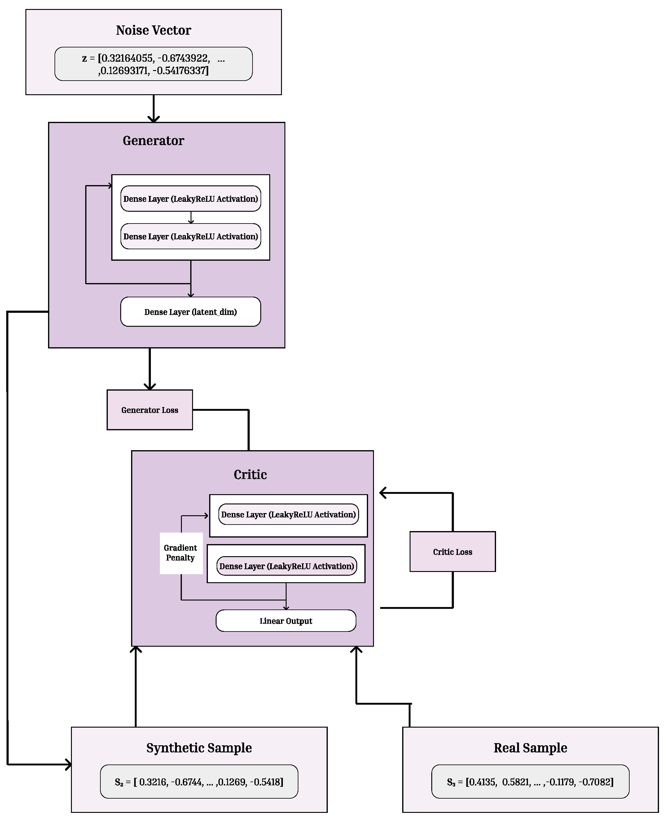
Figure 8.
WGAN-GP Model Architecture The architecture begins with a random noise vector sampled from a latent distribution, which is transformed by the generator through successive dense layers to produce synthetic samples. These generated samples, along with real samples from the dataset, are evaluated by the critic network. The critic computes a Wasserstein distance–based loss and applies a gradient penalty to maintain Lipschitz continuity. The generator is updated to produce samples that the critic cannot distinguish from real data, progressively improving the realism of the synthetic embeddings.
Figure 9.
Diffusion Architecture. (A) A real embedding is passed into the (B) forward noising process, in which Gaussian noise is added to input samples to corrupt them. (C) A noised sample is outputted from this noising process and passed into a (D) reverse noising process, in which noise is gradually removed to reveal synthetic malware samples that closely resemble real malware samples. A U-Net is used to remove this noise. (E) Final vectors of length 104 are outputted from the Diffusion model.
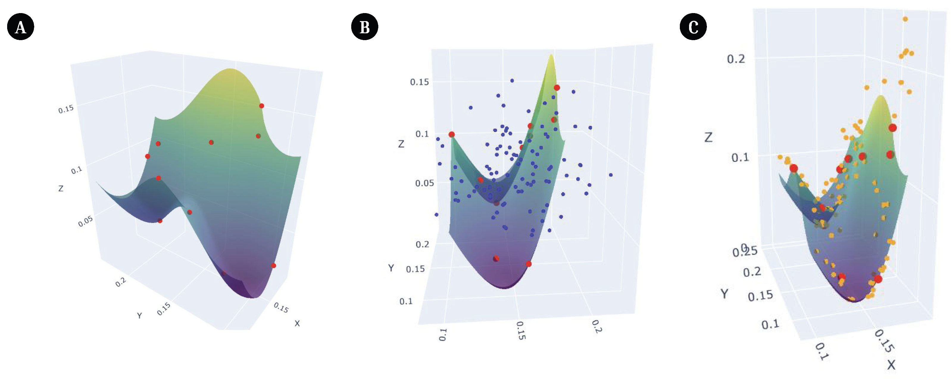
Figure 10.
Manifolds Plots. This plot visualizes a selection of points from (A) Node2Vec output embeddings, (B) Diffusion noise, and (C) CT-Diff noise. This figure is a largely simplified version of the original data. For illustration purposes, it only visualizes 3 of the 120 original dimensions of the Node2Vec embeddings and 10 of its original data points. (A) The first three dimensions of 10 Node2Vec output embeddings are visualized as red points plotted in 3D space and a manifold is created to connect them. The manifold is visualized as the green and blue curved plane. (B) Diffusion noises samples using a normal Gaussian distribution. This is simulated through the blue dots. This noise largely falls outside of the manifold because the original data does not follow a normal distribution. (C) CT-Diff samples noise from the original distribution. Its noise is visualized using orange points, and they fall on or close to the original data’s manifold.
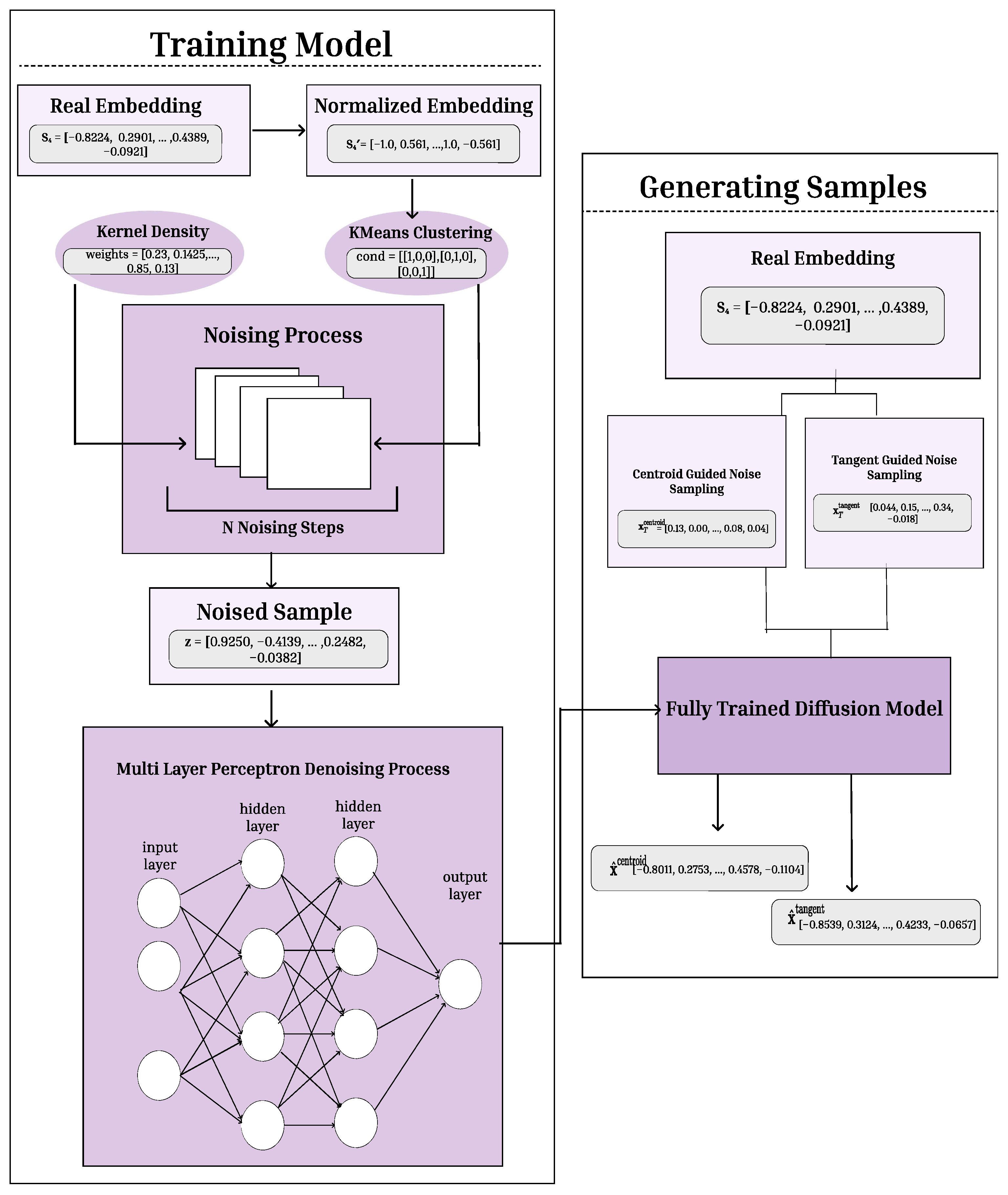
Figure 11.
Cluster-Tangent Model Architecture. This diagram details the sampling process in both Cluster Guided and Tangent Guided Diffusion methods. The training segment builds the full trained diffusion model by applying noise to normalized embeddings and learning to denoise them with denoising MLP. KMeans clustering and KDE guide the noising process. In the generation phase synthetic embeddings are created by sampling noise from either centroid guided or tangent guided noise, then denoised using the trained diffusion model.
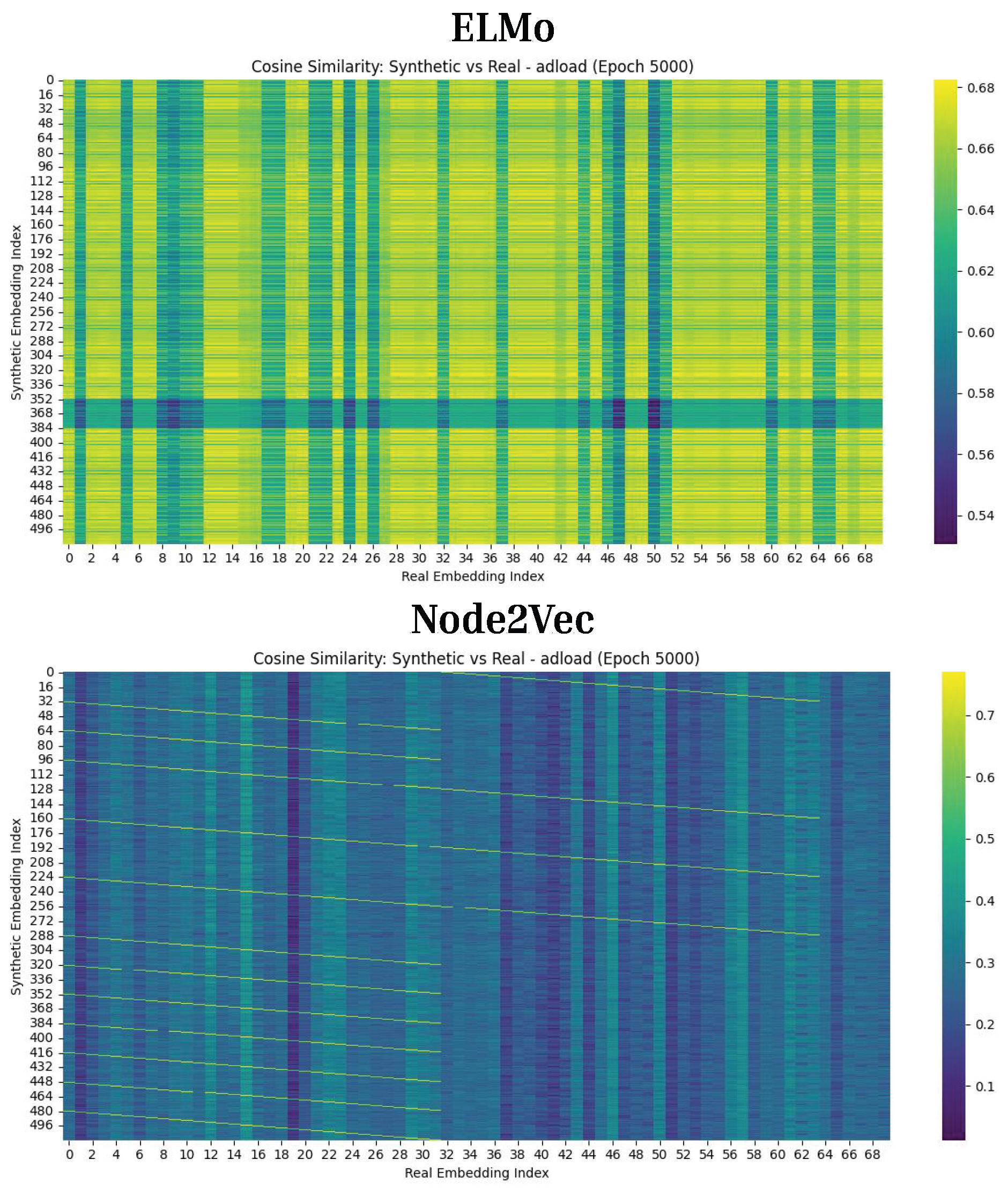
Figure 12.
Cosine Similarity Results for Diffusion The cosine similarity results are shown for Epoch 5000 for the Adload malware family for ELMo and Node2Vec. ELMo achieved a maximum cosine similarity of 0.68, while Node2Vec achieved a maximum cosine similarity of around 0.7. This indicates that using graph embedding techniques with Diffusion yields synthetic malware that more closely aligns with the original data.
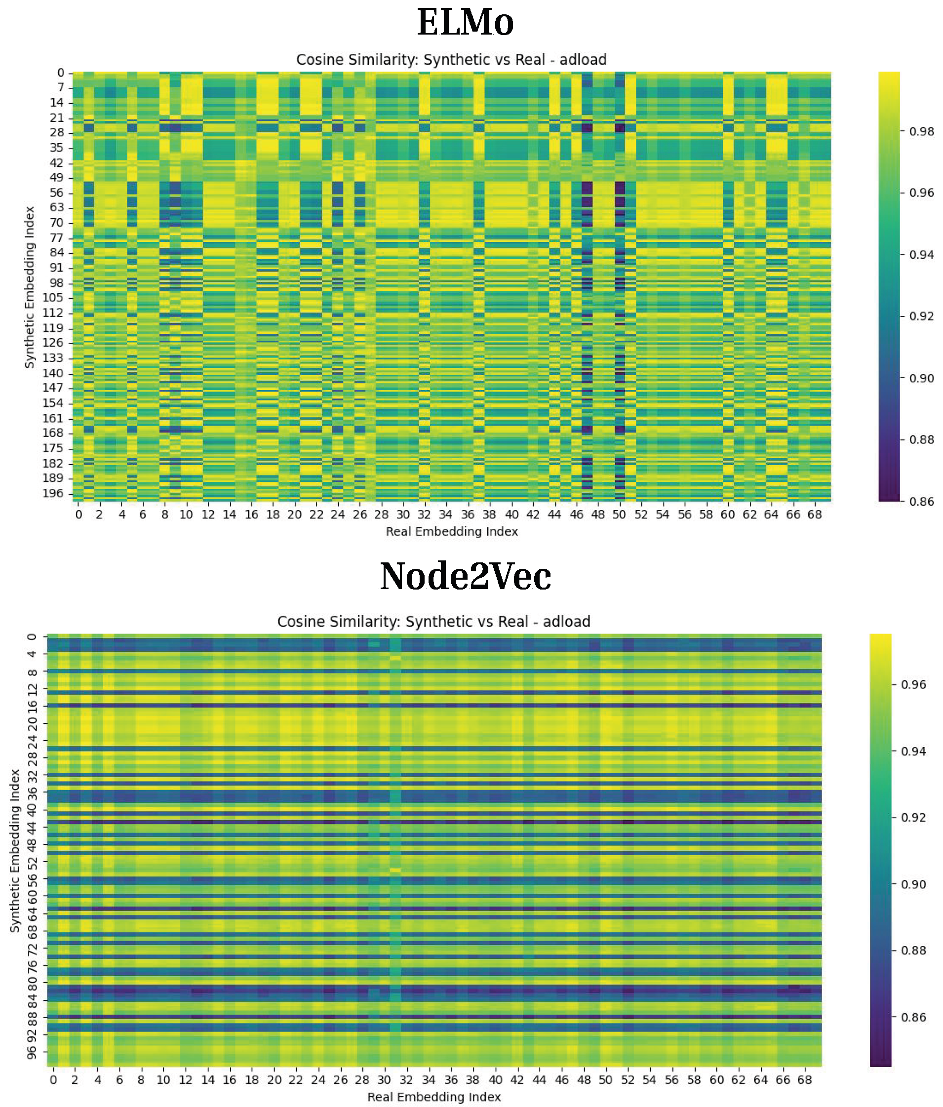
Figure 13.
Cosine Similarity Results for CT-Diff. This figure presents cosine similarity for CT-generated ELMo and Node2Vec embeddings. The light colors in the heatmap indicate consistently high (0.98) similarity across most samples, with occasional dark streaks where similarity dips to 0.86. These results indicate strong generated samples.
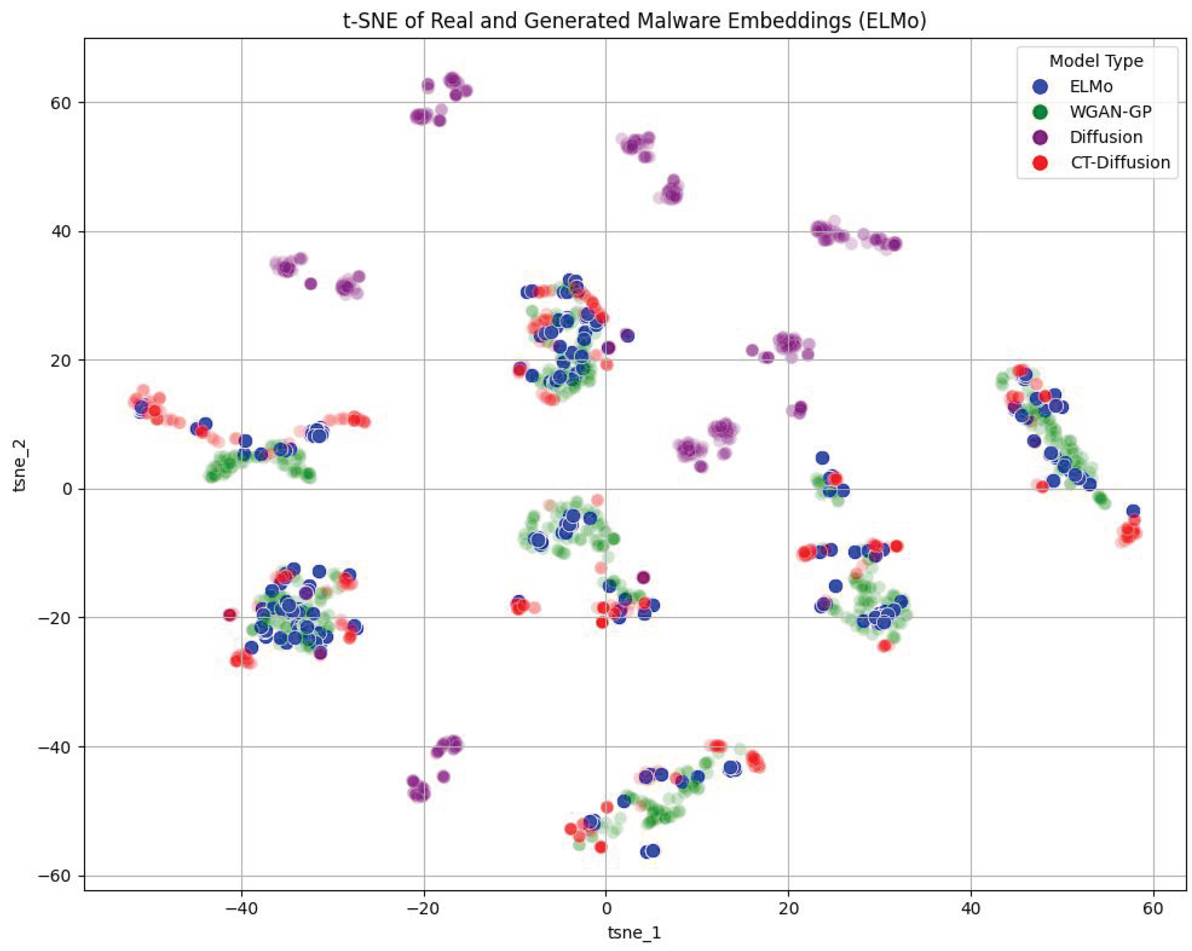
Figure 14.
t-SNE Results for ELMo. This figure displays the t-SNE results with the original ELMo embeddings and the synthetic malware generated by WGAN-GP, Diffusion, and CT-Diff. The CT-Diff embeddings closely follow the original ELMo embeddings, with WGAN-GP performing similarly. Diffusion clusters, but its embeddings do not align well with those of the ELMo embeddings.
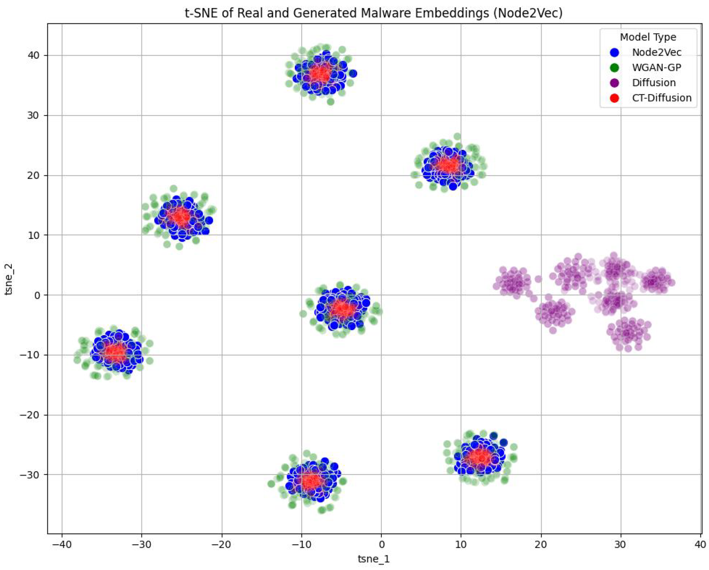
Figure 15.
t-SNE Results for Node2Vec. This figure displays the t-SNE results with the original Node2Vec embeddings and the synthetic malware generated by WGAN-GP, Diffusion, and CT-Diff. The Diffusion syntheticsamples form strong clusters but are not close to the original data. The CT-Diff clusters depict how CT anchors generation to the create stronger generations. WGAN-GP performs similarly.
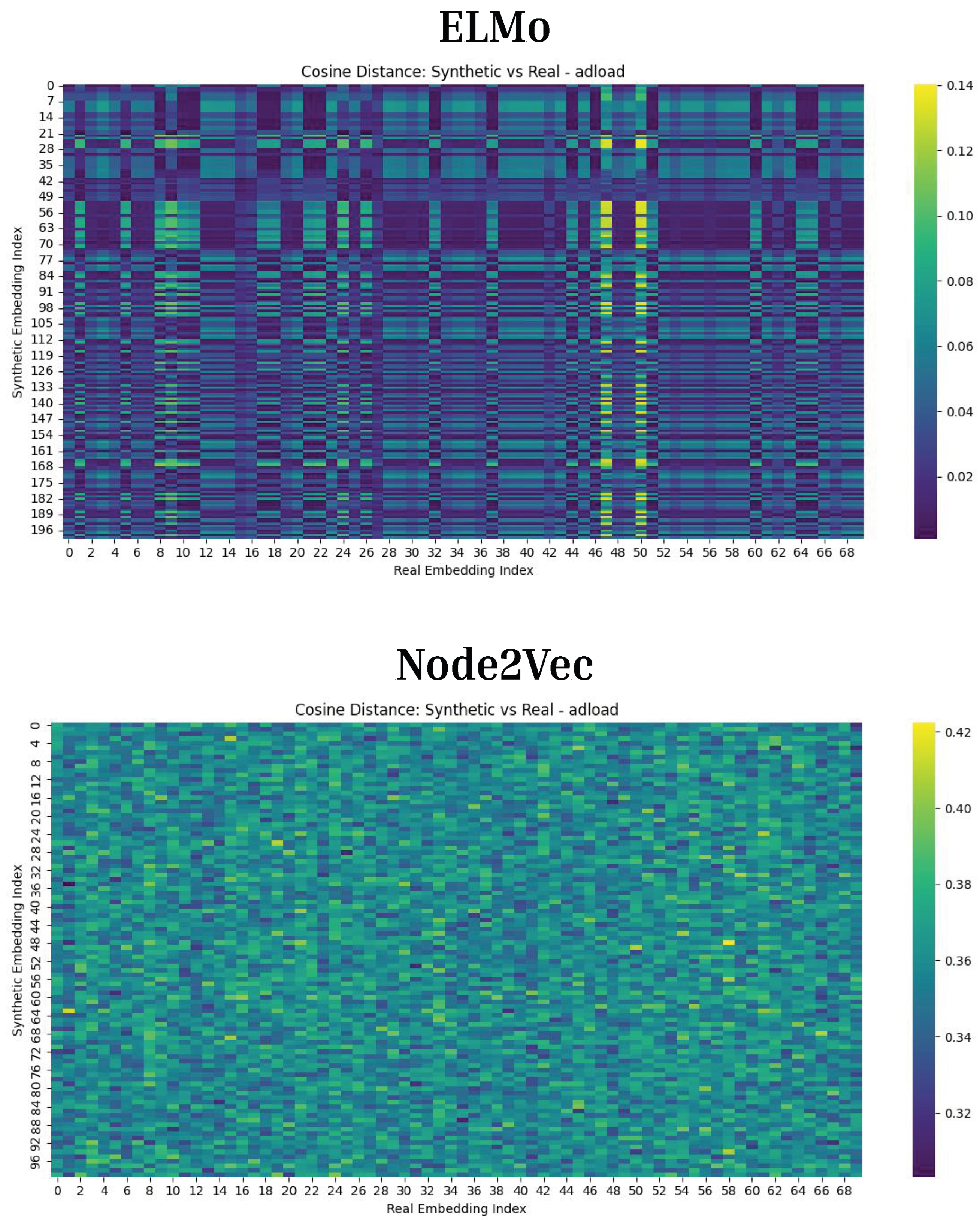
Figure 16.
Cosine Distance Results for CT-Diff This figure shows the results of running Cosine Distance on the synthetic malware samples generated by CT-Diff for ELMo and Node2Vec. For Adload, ELMo achieves a mean cosine distance of 0.0330, while Node2Vec achieves a mean cosine distance of 0.3595. This indicates that generated samples are similar to the original embeddings.
Table 1.
Literature Review and Identified Gaps.
Table 1.
Literature Review and Identified Gaps.
| Study (Author, Year, Title) | Topic | Findings/Gap |
|---|
| Kale et al. [16], Malware classification with Word2Vec, HMM2Vec, BERT, and ELMo | Opcode embeddings for classification | Strong accuracy with BERT on opcode data; lacks generative modeling or data-scarcity augmentation. |
| Aggarwal & Di Troia [17], Malware Classification Using Dynamically Extracted API Call Embeddings | Dynamic API sequence embeddings | Effective for classification; no synthetic data generation or manifold-guided diffusion. |
| Maniriho et al. [18], API-MalDetect: Automated malware detection framework for Windows | Deep learning-based detection of malware attacks | Robust detection pipeline; focuses only on classification, not sample generation. |
| Amer & Zelinka [19], Contextual understanding of API call sequence | Dynamic API analysis | Captures temporal dependencies; lacks embedding optimization or synthetic augmentation. |
| Qiao et al. [20], MLP + Word2Vec for IoT malware classification | Word2Vec for IoT malware | Strong accuracy with static embeddings; no autoencoder or generative refinement. |
| Yesir & Soğukpınar [21], Malware detection and classification using FastText and BERT | NLP-based embeddings | High detection accuracy; lacks diffusion or manifold-aware synthesis. |
| Tran & Di Troia [22], Word Embeddings for Fake Malware Generation | Embedding-driven malware generation | Demonstrated feasibility of fake sample generation; not manifold- or cluster-conditioned. |
| Bao et al. [4], Generating Synthetic Malware Samples using Generative AI against Zero-day Attacks | Use of Word2Vec, GAN, WGAN-GP, and Diffusion to generate synthetic malware | Diffusion improved F1 scores; limited to opcode data; lacks embedding optimization and structure awareness. |
| Mollah et al. [23], Control Flow Graphs, Node2Vec, and GCN Integration | Graph embeddings for malware detection | Captured graph structure well; no generative malware synthesis. |
| McLaren et al. [24], GAN-based malware generation using behavioural graphs | Graph-based GAN generation | Effective structure modeling; GAN prone to mode collapse; lacks manifold-guided refinement. |
| Wesego [25], Graph Representation Learning with Diffusion Generative Models | Diffusion for graph embeddings | Highlights diffusion’s promise; not applied to malware or data-scarce environments. |
| Lee & Choi [26], Local Manifold Approximation and Projection (LoMAP) | Manifold-aware diffusion | Improves generation fidelity via local manifolds; not used for malware embeddings. |
| Chung et al. [27], Improving diffusion models for inverse problems using manifold constraints | Manifold-regularized diffusion | Improves reconstruction quality; no evaluation on malware embeddings. |
| He et al. [28], Manifold Preserving Guided Diffusion | Structure-preserving diffusion | Preserves data geometry; lacks application to malware or low-data scenarios. |
Table 2.
API Call Dataset.
Table 2.
API Call Dataset.
| Malware Family | Samples | Max API Seq. Length |
|---|
| Adload | 70 | 198 |
| Bancos | 71 | 1006 |
| OnlineGames | 70 | 714 |
| Vbinject | 70 | 17,364 |
| Vundo | 71 | 3918 |
| WinWebSec | 70 | 3406 |
| Zwangi | 70 | 772 |
Table 3.
Sample function calls for each malware sample.
Table 3.
Sample function calls for each malware sample.
| Sample Number | Sample Calls | Sample Length |
|---|
| ‘virtualallocex’, ‘getmodulehandle’, ‘freelibrary’ | 3 |
| ‘VirtualAllocEx’, ‘QuerySystemInformation’, …, ‘FreeLibrary’, ‘TerminateProcess’ | 76 |
| ‘LdrFindEntryForAddress’, ‘GetModuleHandle’, …, ‘OpenProcessToken’, ‘VirtualAllocEx’ | 174 |
| ‘CreateThread’, ‘ResumeThread’, …, ‘LdrFindEntryForAddress’, ‘GetModuleHandle’ | 17,364 |
Table 4.
FastText Dimension Experimentation.
Table 4.
FastText Dimension Experimentation.
| Dimension | F1 Score |
|---|
| 88 | 0.97115 |
| 104 | 0.97022 |
| 120 | 0.96108 |
Table 5.
BERT Autoencoder Hyperparameters for Embedding Dimensionality Reduction.
Table 5.
BERT Autoencoder Hyperparameters for Embedding Dimensionality Reduction.
| Parameter | Value |
|---|
| Encoder Architecture |
| Dense Layer 1 | 256 units, ReLU activation |
| Dense Layer 2 | 128 units, ReLU activation |
| Bottleneck Layer | 104 units, Linear activation |
| Decoder Architecture |
| Dense Layer 1 | 128 units, ReLU activation |
| Dense Layer 2 | 256 units, ReLU activation |
| Output Layer | 768 units, Linear activation |
| Training Configuration |
| Optimizer | Adam |
| Loss Function | Mean Squared Error (MSE) |
| Batch Size | 8 |
| Epochs | 200 |
| Validation Split | 0.2 |
| Early Stopping | Patience = 10 (restore best weights) |
| Train/Validation/Test Split | 80%/10%/10% |
Table 6.
BERT Dimension Experimentation.
Table 6.
BERT Dimension Experimentation.
| Dimension | F1 Score |
|---|
| 768 | 0.90632 |
| 104 | 1.00000 |
Table 7.
ELMo Dimension Experimentation.
Table 7.
ELMo Dimension Experimentation.
| Dimension | F1 Score |
|---|
| 1024 | 0.90718 |
| 104 | 1.00000 |
Table 8.
Graph Embedding F1 Scores by Embedding Dimension.
Table 8.
Graph Embedding F1 Scores by Embedding Dimension.
| Embedding Dimension | Graph Embedding F1 Score |
|---|
| 88 | 0.96 |
| 104 | 0.96 |
| 120 | 0.98 |
Table 9.
WGAN-GP hyperparameters.
Table 9.
WGAN-GP hyperparameters.
| Parameter | WGAN-GP Value |
|---|
| Generator |
| Activation | LeakyReLU |
| Hidden Layer 1 | 128 units |
| Hidden Layer 2 | 64 units |
| Hidden Layer 3 | 32 units |
| Batch Normalization | Enabled (momentum = 0.8) |
| Discriminator/Critic |
| Activation | LeakyReLU () |
| Hidden Layer 1 | 128 units |
| Hidden Layer 2 | 64 units |
| Gradient Penalty () | 10 |
| Training Configuration |
| Optimizer | Adam |
| Learning Rate | 0.0001 |
| Betas | (0.5, 0.9) |
| Batch Size | 64 |
| Training Epochs | 2000 |
| Early Stopping | Patience = 100 epochs, |
| Train/Validation/Test Split | 80%/10%/10% |
Table 10.
Diffusion hyperparameters.
Table 10.
Diffusion hyperparameters.
| Parameter | Details |
|---|
| Forward Diffusion |
| Time Schedule | Cosine (), 1000 timesteps |
| Channels | 32 |
| Channel Multipliers | (1, 2, 4, 8) |
| Reverse Diffusion |
| Layers | 4 encoding, 4 decoding |
| Base Width | 64 |
| Attention Heads/Dim Head | 4/32 |
| Activation | Sigmoid Linear Unit (SiLU) |
| Normalization | RMSNorm |
| Training Configuration |
| Optimizer | Adam |
| Learning Rate | |
| Betas | (0.9, 0.99) |
| EMA Decay | 0.995 |
| Gradient Accumulation | 2 steps |
| Batch Size | 64 |
| Total Steps | 8000 |
| Train/Validation/Test Split | 80%/10%/10% |
Table 11.
CT-Diff hyperparameters.
Table 11.
CT-Diff hyperparameters.
| Parameter | Details |
|---|
| Forward Diffusion |
| Time Schedule | Cosine (), 1000 timesteps |
| Reverse Diffusion (MLP Model) |
| Hidden Layers | 3 fully connected layers |
| Hidden Size | 256 units per layer |
| Activation | ReLU |
| Training Configuration |
| Optimizer | Adam |
| Learning Rate | |
| Epochs | 1000 |
| Loss Function | MSE + |
| Train/Validation/Test Split | 80%/10%/10% |
| Density Estimation (KDE) |
| Kernel Function | Gaussian |
| Bandwidth | 0.5 |
| Tangent-Guided Sampling |
| k (Nearest Neighbors) | 10 (for local PCA) |
| Tangent Noise Scale | 0.2 along local tangent direction |
| Drift Noise Mix | 0.85 tangent + 0.15 orthogonal |
| Center Pull Factor | 0.05 toward mean prediction |
Table 12.
WGAN-GP Multiclass Classification F1 Scores.
Table 12.
WGAN-GP Multiclass Classification F1 Scores.
| Embedding Type | RF | SVM | MLP |
|---|
| Train: 100% Real—Test: 100% Fake |
| FastText | 0.6199 | 1.0000 | 1.0000 |
| ELMo | 0.7983 | 1.0000 | 1.0000 |
| BERT | 0.6592 | 1.0000 | 1.0000 |
| Node2Vec | 0.7858 | 1.0000 | 1.0000 |
| Graph2Vec | 0.5448 | 0.7764 | 0.7736 |
| Train: 80% Real, 20% Fake—Test: 20% Real, 80% Fake |
| FastText | 0.8100 | 1.0000 | 1.0000 |
| ELMo | 0.6417 | 1.0000 | 1.0000 |
| BERT | 0.8069 | 1.0000 | 1.0000 |
| Node2Vec | 0.7831 | 1.0000 | 1.0000 |
| Graph2Vec | 0.6682 | 1.0000 | 1.0000 |
| Train: 100% Fake—Test: 100% Real |
| FastText | 0.6628 | 0.9818 | 0.9837 |
| ELMo | 0.6788 | 0.9980 | 1.0000 |
| BERT | 0.6109 | 1.0000 | 1.0000 |
| Node2Vec | 0.7666 | 1.0000 | 1.0000 |
| Graph2Vec | 0.4224 | 0.6965 | 0.7435 |
Table 13.
Diffusion Multiclass Classification F1 Scores.
Table 13.
Diffusion Multiclass Classification F1 Scores.
| Embedding Type | RF | SVM | MLP |
|---|
| Train: 100% Real—Test: 100% Fake |
| FastText | 0.5040 | 0.9571 | 0.9595 |
| ELMo | 0.4531 | 0.6730 | 0.7378 |
| BERT | 0.5600 | 0.9335 | 0.9877 |
| Node2Vec | 0.6929 | 0.9812 | 0.9676 |
| Graph2Vec | 0.0357 | 0.9382 | 0.9837 |
| Train: 80% Real, 20% Fake—Test: 20% Real, 80% Fake |
| FastText | 0.6068 | 0.9980 | 1.000 |
| ELMo | 0.7966 | 1.000 | 1.000 |
| BERT | 0.7638 | 1.000 | 1.000 |
| Node2Vec | 0.6920 | 1.000 | 1.000 |
| Graph2Vec | 0.5724 | 0.9980 | 1.000 |
| Train: 100% Fake—Test: 100% Real |
| FastText | 0.7280 | 0.8658 | 0.9649 |
| ELMo | 0.8068 | 0.2115 | 0.9979 |
| BERT | 0.8080 | 0.0354 | 1.000 |
| Node2Vec | 0.7805 | 0.8526 | 0.9788 |
| Graph2Vec | 0.5451 | 0.9192 | 0.9772 |
Table 14.
CT-Diff Multiclass Classification F1 Scores.
Table 14.
CT-Diff Multiclass Classification F1 Scores.
| Embedding Type | RF | SVM | MLP |
|---|
| Train: 100% Real—Test: 100% Fake |
| FastText | 0.8025 | 1.0000 | 1.0000 |
| ELMo | 0.8270 | 1.0000 | 1.0000 |
| BERT | 0.6851 | 1.0000 | 1.0000 |
| Node2Vec | 0.8095 | 1.0000 | 1.0000 |
| Graph2Vec | 0.8137 | 1.0000 | 1.0000 |
| Train: 80% Real, 20% Fake—Test: 20% Real, 80% Fake |
| FastText | 0.8095 | 1.0000 | 1.0000 |
| ELMo | 0.6287 | 1.0000 | 1.0000 |
| BERT | 0.7098 | 1.0000 | 1.0000 |
| Node2Vec | 0.8071 | 1.0000 | 1.0000 |
| Graph2Vec | 0.8117 | 1.0000 | 1.0000 |
| Train: 100% Fake—Test: 100% Real |
| FastText | 0.6126 | 0.9959 | 0.9838 |
| ELMo | 0.7458 | 1.0000 | 1.0000 |
| BERT | 0.6229 | 1.0000 | 1.0000 |
| Node2Vec | 0.5540 | 1.0000 | 1.0000 |
| Graph2Vec | 0.8079 | 1.0000 | 1.0000 |
