Abstract
In this paper, the dynamics of long payload transportation via two bridge cranes in three dimensions is studied. The position of the cranes is known, and it is used as a kinematic coercion. Using the independent variables, equations of motion are derived. Two types of crane motion are considered: the Cubic Spline Trajectory (CST) and the trapezoidal one. Numerical simulations are compared with experimental results from the literature on the long payload moving in one plane. Qualitatively similar results were obtained. The anti-swing control is verified and compared with each function of the motion. The difference between the distance of the cranes’ bridge and payload’s anchorage length is considered. It does not reveal any relevant improvement of the anti-swing cargo control. The considered model can be used in the anti-swing wind excitation control system in future work. Also, this work can be used to investigate the energy harvesting system in long payload transportation.
1. Introduction
Transportation machines such as bridge cranes are commonly used in many branches of industry. The anti-swing control problem is well known and described only for payloads considered as a spherical pendulum [1,2,3,4,5,6,7,8,9,10,11,12,13,14]. The cargo measuring a significant length has to be transported by using two cranes, for example, aircraft components, a railway wagon, long steel pipes, prefabricated concrete elements and other bulky loads [7,14].
In [3], a review of crane models and control systems available in the literature is conducted. The authors discuss the above problems and their applications and limitations. The crane model is analyzed by using the multiple scales method. In [1,2], the same method as above is applied.
Blajer in [5] presented an effective numerical code to solve the equation of motion, using the backward Euler method. Then, the obtained feedforward control law is enhanced by a closed-loop control strategy in the presence of perturbation.
Another control method is shown in [7]. The problem of the anti-sway system was solved using the pole placement method. The crane system is considered a linear model.
A machine learning-based control method for overhead cranes is introduced in [15] that avoids a reliance on precise system models. A learning term replaces traditional sliding mode control to eliminate chattering and improve the convergence speed. A disturbance observer enhances the robustness against uncertainties.
In [6], the dynamics of the payload are presented as a double spherical pendulum. Such a model enables us to obtain a more significant control method.
Also, ref. [16] presents nonlinear dynamic models of a double-pendulum overhead crane transporting a distributed-mass payload (DMP), both with and without hoisting. The influence of cable length and payload parameters on hook and payload oscillations is analyzed through simulations and validated by experiments. The results confirm that the models accurately capture the system’s dynamics and can support the development of effective control strategies to reduce DMP oscillations.
Currently, different solutions for long cargo transportation are being sought. In [17], a transport with a team of two robots is proposed, and nonlinear attractor dynamics are used as the control system.
Grabski and Strzako present in [18] a model of the phenomena occurring before the charge is detached from the ground. The results revealed the phenomenon of solution bifurcation due to friction.
A very deep analysis of the crane motion function is performed in [12]. The authors focused on two types of functions: the Curve Spline Trajectory (CST) and the trapezoidal one.
A challenging issue is the coupled operation of two cranes in order to transport long payloads, such as, e.g., long steel products. The transportation of long payloads using coupled crane operations is considered extremely dangerous. The confirmation of this one can be found among others in [19], where the author wrote, “Bridge cranes are probably the most dangerous piece of equipment used to handle long steel products, because even the crane’s smallest movements are magnified by the long payload”.
Two cranes can operate synchronized in the movements of the girder and carriage, respectively. To ensure the safety of the transportation, usually only one mechanism (travelling or traversing) is used; lateral movements of the load (perpendicular to the direction of movement) are also unavoidable, for example, due to the mutual displacement of the points of attachment of the ropes of the load, resulting from the inaccuracy of its suspension, or the operation of the mechanism control systems.
Therefore, it is very important to know the behavior of the payload. Furthermore, the publication [20] presents an overview of the existing solutions for gantry drive systems and future research directions, presenting, inter alia, control systems using mathematical models. Therefore, models that effectively describe payload behavior are becoming indispensable in modern control systems, allowing the control of payload movements during the duty cycle.
Deep reinforcement learning (DRL) for the time-optimal control of gantry cranes is explored in [21]. The DRL method reduces transport time by 20% compared to traditional control approaches.
Apart from the single-mass or dual-mass payload models with one rope attachment point that frequently appear in the available literature, one can also find descriptions of systems with two or more attachment points.
For example, in [22], the system of a 3-car crane with a fuzzy PID Controller is presented, and in [23] the authors present, among others, the modelling technique of a container spreader as a bifilar pendulum with a sheave block.
In [9], the transportation in one plane of the long payload suspended in two rope systems is considered, but with the assumption of small oscillation angle values.
The problem of transporting a long payload using two bridge cranes is considered in [24]. The authors point out the lack of scientific research in this area and propose a dynamic model based on six variables, along with a new control method that effectively suppresses payload oscillations.
In the presented paper, the dynamics of the long payload in three dimensions is considered. The model is not restricted to small oscillations, i.e., large spherical displacements are considered. The subject concerns the tandem operation of travelling cranes. This model, using various displacement functions of the rope anchor, enables us to specify the behavior of the payload during working motions. The model is not restricted to only one plane, as presented in [9], but allows us to simulate also the synchronous movement of both crane mechanisms and the behavior of a transported long payload. A mathematical model was derived using three independent variables, with an innovative approach to their selection. The positions of the cranes are known, and they are used as kinematic coercions. The model was verified by comparing the experimental data on cargo motion from [9] with simulation results.
The paper is organized as follows. The assumptions of the long payload model considered are introduced in Section 2. Next, the geometry and dynamics of the system are shown in Section 3. The numerical simulations and their experimental confirmation are contained in Section 4. Finally, the conclusions are presented in Section 5.
2. Nonlinear Model of Long Cargo
The considered system is composed of two bridge cranes and a long payload, as presented in Figure 1. The position of the first rope anchor is marked by point O1, and the second by O2. Both cranes are on the same level. In the considered model, the phenomenon of skewing was omitted due to the complex nature of the payload’s motion description. An ideally rigid structure of the crane was assumed to simplify the analysis. Let x = [x1, x2, y1, y2]T describe the position of the cranes and their trolley. The ropes are weightless and inextensible, with lengths h1 and h2, respectively. The long load is considered as the rod of length b and mass m.
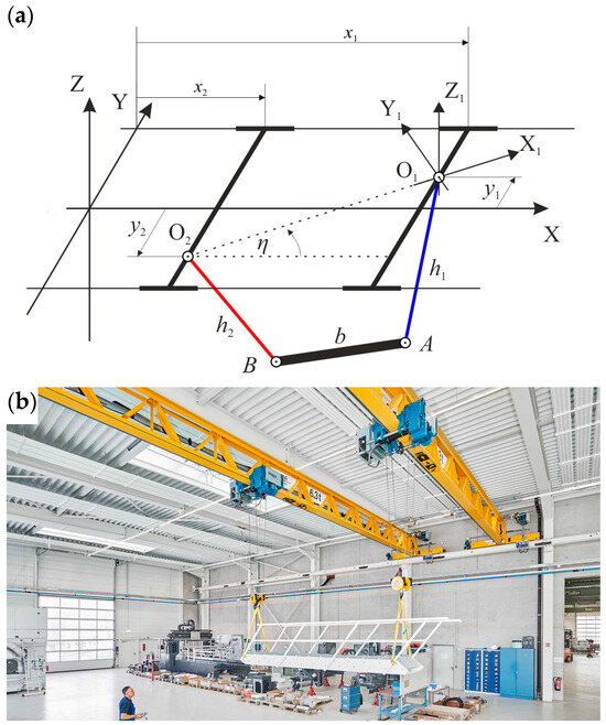
Figure 1.
(a) Model of transportation of long load by two bridge cranes and (b) example of a real system [25].
The inertial reference frame XYZ is placed as in Figure 1a. Let l be the distance between trolleys O1 and O2:
Additionally, let us consider the reference frame X1Y1Z1 which is located at point O1.
This reference frame is translated and rotated to the first one as follows:
where and .
Then, the coordinates of point A in the inertial reference frame XYZ can by presented by the coordinates in the frame X1Y1Z1, as follows:
It is easier to show the geometry of the system with respect to a frame of reference, X1Y1Z1. Then, after the transformation, which is shown above in Equations (2) and (3), the coordinates of each point of the system in the inertial reference frame XYZ may be obtained.
In this paper, the payload is looked upon as a rigid body. The considered system has three degrees of freedom; there are three independent variables needed.
2.1. Geometry of the Long Payload
In this section, the Cartesian coordinates of the load ends are derived. The main problem is how to choose independent variables. In many different papers, the spatial quadrangle is described by Lagrange multipliers using bond equations [26]. Point A can be obtained by angles α and β, like the spherical pendulum, where α is the angle between |O1A| and the Y1Z1 plane and β is the rotation angle of |O1A| about the X1 axis. The coordinates of point A in a reference frame X1Y1Z1 are given by the following formula:
To obtain the position of point B, divide the space between the rod and the suspension into two triangles, ΔAO1O2 and ΔABO2, which are depicted in Figure 2. The angle θ between them is the third independent variable.
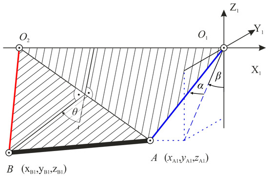
Figure 2.
Three independent variables.
Let us mark the line segment |AO2| as d (see Figure 3). Taking into consideration the cosine theorem, one obtains the following:
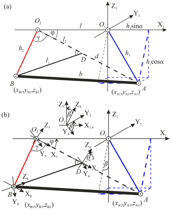
Figure 3.
(a) Geometry of the system; (b) system coordinate transformations.
Marking angle ∠AO1O2 as φ, we obtain the following:
and, marking angle ∠AO2B as γ, then using the cosine theorem, cos γ can be obtained:
The altitude l1 of the triangle ΔABO2 can be obtained as follows:
and crosses |AO2| at point D. Marking |O2D| as l2, then the following is obtained:
Several transformations of the local coordinate system have to be performed to obtain the Cartesian coordinates of point B corresponding to the X1Y1Z1 coordinate system. Let us consider the coordinate system B as follows: the X8 axis is parallel to d, the Z8 axis is perpendicular to d, and the center of this system is in point B, as shown in Figure 3b. First, the system translation from point B to point D by l1 is performed. In the next step, the system X7Y7Z7 rotates by θ around the X7 axis, which is described by the rotation .
Then, the translation from point D to point O2 by l2 along the X6 axis occurs. Furthermore, one rotates the system by φ about the Y5 axis and by β about the X4 axis. Eventually, the system is translated from point O2 to point O1 by l along the X1 axis. Each step is described by the following matrices [26]:
Then, point B can be obtained using the following formula:
After the calculations, the above vector takes the following form:
Finally, using Equations (1)–(18), one may calculate the Cartesian coordinates of points A and B described in the inertial reference frame XYZ, as follows:
2.2. Dynamics of the Long Load
Using the coordinates of points A and B from Equations (1)–(18), one may obtain the Euler angles describing the long load inclination to each axis. We assumed that the center of the mass of the load is in a geometric center (point C). The position of this point is the midpoint of AB. After the calculation of the derivatives of the point C coordinates and the angular velocities, the kinetic energy and potential energy are presented as follows:
where B is the matrix of inertia.
The motion resistance is represented by a viscous damping model, characterized by a proportional relationship to the angular velocity. Since the third variable θ is virtual, it is difficult to accurately model damping in the system such that the motion of both suspensions is damped in the same manner. The energy dissipation function should dampen movement in nodes O1 and O2 equally. Let us consider the new variables to describe the coordinates of points A and B in frame X1Y1Z1 in the same manner: α1 = α, β1 = β and α2, β2. Then, point B can be described by following formula:
Comparing (18) to (20), one can receive the following:
After obtaining the derivatives and from Equation (21), the damping function takes the following form:
where and are the viscous damping coefficients.
Based on Equations (18)–(22) and the Lagrange equation of the second type, one can derive three coupled second Ordinary Differential Equations (ODEs). By applying the substitutions described in Equations (1)–(22), a system of equations is obtained that depends only on α, β, θ, geometric parameters, and the given displacements of the trolleys x1, y1, x2, y2 and their derivatives. It can be written using the mass matrix M, the damping vector D and the vector of rest R:
where q = [α, β, θ]T and x = [x1, x2, y1, y2]T.
Due to the complexity of the explicit form of the above equations, it will not be presented (for shortness) [26]. The ODEs describing the motion of the long payload have been integrated using the Runge–Kutta–Fehlberg method (RKF45).
2.3. Crane Motion Function
The main task of the crane operation is to move the payload from one place to another. The motion of the crane can be optimized with respect to the time and payload swing [1,2,3,4,5,6,7,8,9,10,11,12,13,14]. Most papers concern an anti-swing control of the payload. This problem is solved by setting the motion time to be adequate to the swing period of the payload. Usually, the motion consists of three phases: an acceleration period (Ta), a steady motion period (Ts) and a breaking period (Tb).
In this paper, it is assumed that Ta is equal to Tb. The period Ts can be calculated as the difference between the total time of motion T and 2Ta. In [12], two types of crane motion functions were presented, the Cubic Spline Trajectory (CST) and the trapezoidal, which were used to transport a long load in one plane.
In CST, the crane motion is described by the following general formulas:
where t is time, j is jerk and , and are the initial conditions. The values of the initial conditions and sign of j depend on the moment of movement (½Ta, Ta, Ts, ½Tb, Tb).
The value of the latter can be obtained from the maximum acceleration and velocity of the crane and the above motion function. The value of j affects the acceleration value. Moreover, acceleration is limited due to a possible slip in a specific mechanism. The exemplary crane motion described by Equation (24) is presented in Figure 4a.
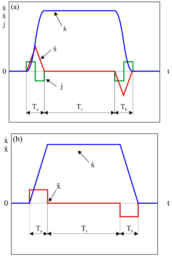
Figure 4.
Two types of crane motion functions: (a) CST and (b) trapezoidal.
Let us consider the trapezoidal motion described by the following equation:
where t is time, a is the acceleration value and and are the initial conditions. As before, a can be calculated from the maximum acceleration and velocity of the crane. The exemplary crane motion described by Equation (25) is depicted in Figure 4b.
The crane motion functions, presented in Equations (24) and (25), are applied in numerical simulations of the investigated system.
3. Numerical Simulations
In simulations, the following were considered: the hoisting rope length h1 = h2 = 5.5 [m], the mass of the load m = 565 [kg] and the length b = 4.0 [m]. The same values of the parameters were applied in the experiment in [9] for motion in one plane. Based on their results, the damping coefficients cf1 and cf2 in Equation (22) are adjusted, so the damping decrement of α equals 0.083 and β equals 0.041. The time series of the damped oscillations in one direction are presented in Figure 5.
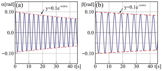
Figure 5.
Time series of damped oscillations of (a) α and (b) β.
Two types of cranes motion are considered: CST and trapezoidal. In both cases, it is assumed that the maximum velocity of each crane is equal to 0.3 [m s−1] and the total time of motion T is equal to 40 [s]. The best results of the payload anti-swing control can be obtained when T is equal to the multiplicity of the natural period of the system [9,11,12]. For short rope oscillation periods, it is very small and caused acceleration, higher than what is acceptable due to non-slip. For a higher multiplicity, the oscillation amplitude is lower, and the acceleration can be lower. The considered long payload suspended on two ropes has different eigenfrequencies for α and β, which can be observed in Figure 5. Thus, the coefficients in Equations (24) and (25) have to be calculated separately for each direction of the crane and the trolley motion.
Comparison of CST with the Trapezoidal Motion Function
Let us compare both motion functions with each other. The distance l between the trolleys is equal to the cargo anchorage b = 4.0 [m]. Let us consider the same cranes’ motion but only in the X axis direction ((t) = (t) and 1(t) = 2(t) = 0).
In the subsequent simulation, the following initial conditions were considered:
x1(0) = 0, x2(0) = −4, y1(0) = y2(0) = 0, (0) = (0) = 0, 1(0) = 2(0) = 0, α(0) = β(0) = θ(0) = 0, (0) = (0) = 0.
The directions of both horizontal movements are perpendicular. If both cranes have the same motion, then the payload will not spin around the Z axis. The control of one mechanism influences the velocity and load displacement only in one vertical plane, whereas the other mechanism is responsible for the payload motion in the other perpendicular vertical plane. It is often assumed that both mechanisms are independent in relation to each other, that is, the movement of the cargo in one plane does not influence the cargo in the movement of the other one [9,11,12].
Let us assume that the time acceleration is a multiplicity of a natural period of the load (for α): Ta = Tα [s], Ta = 2Tα [s] and Ta = 3Tα [s]. In Figure 5, the time series of the cranes’ velocity = , and that of angle α is presented. We are only interested in the motion of the cranes with the lowest payload oscillations.
In Figure 6, if Ta equals Tα, then the oscillations of the payload will be much higher during the whole transportation than the other multiplicity of Tα. The lowest sway is with the obtained acceleration period Ta = 2Tα. There is only one swing, and after that the oscillations are completely suppressed during the steady motion period and also after the crane stops.
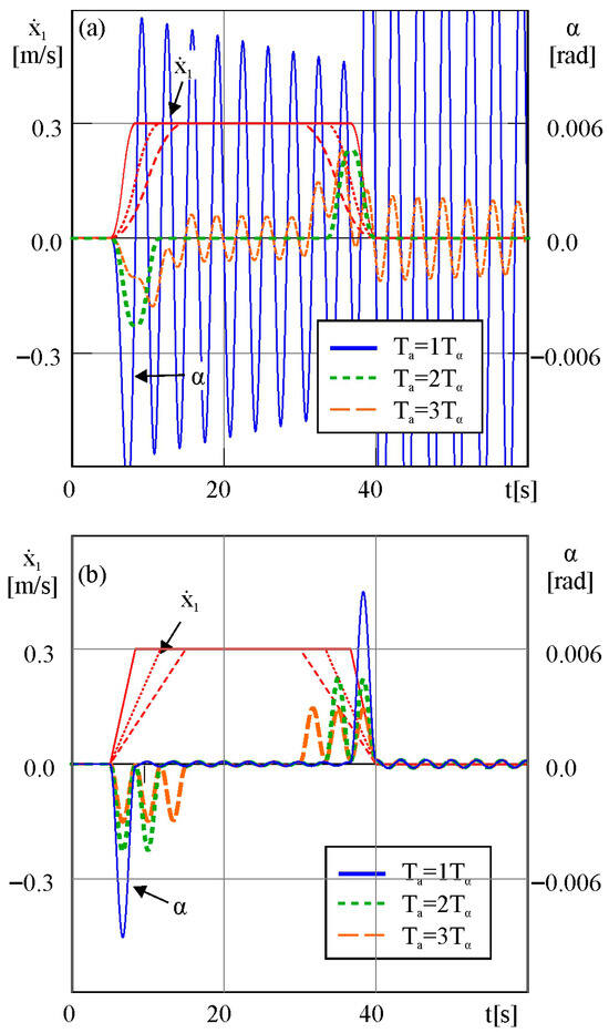
Figure 6.
Time series of cranes’ velocity = (red lines), and of angle α with Ta = Tα (solid blue line), Ta = 2Tα (dotted green line) and Ta = 3Tα (orange dashed line) in different motion functions: (a) CST and (b) trapezoidal.
If the trapezoidal motion function is considered, then the vibrations of the cargo will be very small (α ≈ 0.0004 rad, what is equal 2.2 [mm]) during the steady motion. This result does not depend on the multiplicity period (the amplitude of oscillations is the same for all considered multiplicities), which may be seen in Figure 6b. The differences between them are in the swing amplitude during the acceleration and braking periods and the crane acceleration.
The CST motion function damps the payload oscillation only for Ta = 2Tα, which can be seen in Figure 6a. The maximum velocity of the crane, whose time acceleration equals 2Tα, is set, then only one value of the maximum crane acceleration will be obtained. The trapezoidal motion function enables one to set the crane acceleration without losing the anti-swing control of the load.
In both cases of the used motion function, qualitatively similar results to those in [9,12] were obtained.
4. Different Distance of Crane Bridges with Constant Load Anchorage
If the distance l between the cranes’ trolleys is greater than the distance b of the load’s anchorage, then the fixed point and period of α will be changed, which is shown in Figure 7. It also results in a change in the angle of inclination of the payload during its swing.
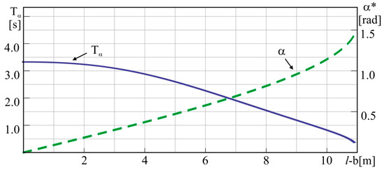
Figure 7.
The change in α fixed point (green dashed line) and α period (blue solid line) versus the difference between the distance between the crane trolleys and the payload anchorage.
Assume the same motion of the cranes ( = and x1 = x2). According to Figure 7, the considered system was investigated with the following differences between the payload length and the crane distance: 0 m, 2 m, 4 m and 6 m. The long payload oscillations after the crane stopped did not change significantly while the considered differences were increasing. It seems to be pointless to use such a spacing between the cranes. Furthermore, when the fixed point of α is changed, then the force in the rope increases.
5. Long Payload Transportation with Perpendicular Fluctuations
In the real environment, cargos are transported in the presence of the wind. Such a situation is presented in many papers. In [11], the wind acts on the load with a changing velocity. If the payload is considered as a spherical pendulum, then the wind disturbs the trajectory of the cargo. If a long payload is assumed, then the wind influences both the trajectory of the center of the mass payload and the rotation around the center of the mass payload. Then, the motion of the long payload is more complex, which is contained in the derived model.
The presented situation is considered in the numerical simulation. The cranes are moving in the X axis direction without delay. After 10 s, the payload is forced in the perpendicular direction due to the motion of the wind. To present the full dynamics of the system, let us consider the eccentric force. In this paper, the model of the long payload is shown, but not the wind excitation model. This study will be conducted in future work. An example of the behavior of the system subjected to wind action is presented below. Therefore, the non-zero initial conditions of velocity and are considered as the wind action.
In Figure 8, the time series of all variables are shown. The above result presents the motion of the payload in 3D. The vibration of θ influences the other variables. The amplitudes of α and β oscillate. The usage of the motion function (Equations (24) and (25)) for anti-swing control is not enough. In future research, a control system based on a closed loop will be created.
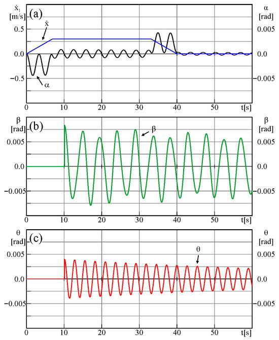
Figure 8.
Time series of (a) velocity , angle α, (b) angle β and (c) angle θ with wind action at 10 s.
6. Conclusions
In this paper, the dynamics of the long payload transportation via two bridge cranes in three dimensions were studied. The positions of the cranes are known, and they are used as a kinematic coercion. By using the independent variables, the equations of motion are derived. Two types of crane motion are considered: the CST and the trapezoidal one. The anti-swing control is qualitatively verified and compared with each function of the motion. The difference between the distance of the bridge of the cranes and the anchorage of the payload is considered. It does not reveal any relevant improvement in the anti-swing payload control. Also, it induces both a change in the α fixed point and the α period.
In subsequent research, the author plans to build an experimental setup with a model of two cranes transporting a long payload. Subsequently, a quantitative verification of the model will be achieved. Next, a detailed analysis of wind excitation will be carried out, followed by the development of a strategy for damping the resulting oscillations. The author also plans to use the model to investigate the potential for energy recovery during the transportation of long payloads.
Funding
This research received no external funding.
Institutional Review Board Statement
Not applicable.
Informed Consent Statement
Not applicable.
Data Availability Statement
The datasets used and analyzed during the current study are available from the corresponding author on reasonable request.
Conflicts of Interest
The author declares no conflicts of interest.
References
- Butler, H.; Honderd, G.; Van Amerongen, J. Model reference adaptive control of a gantry crane scale model. IEEE Control Syst. 1991, 11, 57–62. [Google Scholar][Green Version]
- Chin, C.M.; Nayfeh, A.H.; Mook, D.T. Dynamics and Control of Ship-Mounted Cranes. J. Vib. Control 2001, 7, 891–904. [Google Scholar] [CrossRef]
- Abdel-Rahman, E.M.; Nayfeh, A.H.; Masoud, Z.N. Dynamics and Control of Cranes: A Review. J. Vib. Control 2003, 9, 863–908. [Google Scholar] [CrossRef]
- Ghigliazza, R.; Holmes, P. On the dynamics of cranes, or spherical pendula with moving supports. Int. J. Non-Linear Mech. 2002, 37, 1211–1221. [Google Scholar] [CrossRef]
- Blajer, W.; Kolodziejczyk, K. Dynamics and control of rotary cranes executing a load prescribed motion. J. Theor. Appl. Mech. 2006, 44, 929–948. [Google Scholar]
- Manning, R.; Kim, D.; Simghose, W. Dynamics and Control of Bridge Cranes Transporting Distributed-Mass Payloads. J. Dyn. Syst. Meas. Control 2009, 132, 014505. [Google Scholar] [CrossRef]
- Smoczek, J.; Szpytko, J. Pole Placement Approach to Crane Control Problem. J. Konbin 2010, 14, 235–246. [Google Scholar] [CrossRef]
- Hong, K.S.; Ngo, Q.H. Sliding-Mode Antisway Control of an Offshore Container Crane. IEEE/ASME Trans. Mechatron. 2012, 17, 201–209. [Google Scholar]
- Kosucki, A. Model of a Long Payload Suspended on Two Cooperating Winches and Its Preliminary Experimental Verication. Mech. Mech. Eng. 2017, 21, 569–589. [Google Scholar]
- Fang, Y.; Wang, P.; Sun, N.; Zhang, Y. Dynamics Analysis and Nonlinear Control of an Offshore Boom Crane. IEEE Trans. Ind. Electron. 2014, 61, 414–427. [Google Scholar] [CrossRef]
- Tomczyk, J.; Cink, J.; Kosucki, A. Dynamics of an overhead crane under a wind disturbance condition. Autom. Constr. 2014, 42, 100–111. [Google Scholar] [CrossRef]
- Cink, J.; Kosucki, A. Wybrane metody kształtowania prędkości mechanizmów jazdy w celu minimalizacji wahań ładunku. Probl. Rozw. Masz. Rob. 2015, 51–65. Available online: http://www.kmrnis.p.lodz.pl/files/Monografia_PRMR_AKosucki_2015_JC_AK.pdf (accessed on 1 November 2025).
- Leban, F.A.; Diaz-Gonzalez, J.; Parker, G.G.; Zhao, W. Inverse Kinematic Control of a Dual Crane System Experiencing Base Motion. IEEE Trans. Control Syst. Technol. 2015, 23, 331–339. [Google Scholar] [CrossRef]
- Sun, N.; Fang, Y.; Chen, H. Adaptive antiswing control for cranes in the presence of rail length constraints and uncertainties. Nonlinear Dyn. 2015, 79, 41–51. [Google Scholar] [CrossRef]
- Chen, J.; Shi, R.; Ouyang, H. Data-driven discrete learning sliding mode control for overhead cranes suffering from disturbances. Nonlinear Dyn. 2025, 113, 3357–3372. [Google Scholar] [CrossRef]
- Bello, M.; Mohamed, Z.; Efe, M.; Ishak, H. Modelling and dynamic characterisation of a double-pendulum overhead crane carrying a distributed-mass payload. Simul. Model. Pract. Theory 2024, 134, 102953. [Google Scholar] [CrossRef]
- Machado, T.; Malheiro, T.; Monteiro, S.; Erlhagen, W.; Bicho, E. Attractor dynamics approach to joint transportation by autonomous robots: Theory, implementation and validation on the factory floor. Auton. Robot. 2019, 43, 589–610. [Google Scholar] [CrossRef]
- Grabski, J.; Strzalko, J. Dynamic analysis of the load hoisting process. J. Theor. Appl. Mech. 2003, 41, 853–872. [Google Scholar]
- Alesia, J. Handling Long Steel Products Proves to Be a Balancing Act. Iron Steel Technol.—Saf. First 2011, 38–39. [Google Scholar]
- Ramli, L.; Mohamed, Z.; Abdullahi, A.M.; Jaafar, H.; Lazim, I.M. Control strategies for crane systems: A comprehensive review. Mech. Syst. Signal Process. 2017, 95, 1–23. [Google Scholar] [CrossRef]
- Zhong, J.; Nikovski, D.N.; Yerazunis, W.S.; Ando, T. Learning Time-Optimal Control of Gantry Cranes. In Proceedings of the 2024 International Conference on Machine Learning and Applications, Vienna, Austria, 21–17 July 2024; IEEE: New York City, NY, USA, 2024; pp. 945–950. [Google Scholar] [CrossRef]
- Yildirim, Ş.; Gordebil, A. Sway Control of 3-Cars Crane System Using Proposed Fuzzy-PID Controller. Recent Innov. Mechatron. 2020, 7, 1–8. [Google Scholar] [CrossRef] [PubMed]
- Cibicik, A.; Myhre, T.A.; Egeland, O. Modeling and Control of a Bifilar Crane Payload. In Proceedings of the 2018 Annual American Control Conference (ACC), Milwaukee, WI, USA, 27–29 June 2018; pp. 1305–1312. [Google Scholar] [CrossRef]
- Huang, J.; Zhu, K. Dynamics and control of three-dimensional dual cranes transporting a bulky payload. Proc. Inst. Mech. Eng. Part C J. Mech. Eng. Sci. 2020, 235, 1956–1965. [Google Scholar] [CrossRef]
- Demag Cranes & Components GmbH. Available online: https://www.demagcranes.com/sites/default/files/blog_images/2022/09/Manuf-2-cranes.jpg (accessed on 23 October 2025).
- Witkowski, B. Modeling of the dynamics of two coupled spherical pendula. Eur. Phys. J.—Spec. Top. 2014, 223, 631–648. [Google Scholar] [CrossRef]


Disclaimer/Publisher’s Note: The statements, opinions and data contained in all publications are solely those of the individual author(s) and contributor(s) and not of MDPI and/or the editor(s). MDPI and/or the editor(s) disclaim responsibility for any injury to people or property resulting from any ideas, methods, instructions or products referred to in the content. |
© 2025 by the author. Licensee MDPI, Basel, Switzerland. This article is an open access article distributed under the terms and conditions of the Creative Commons Attribution (CC BY) license (https://creativecommons.org/licenses/by/4.0/).