Article

Ship Traffic Flow Analysis and Prediction in High-Traffic Areas Under Complex Environments

by
Liulu Luo
1,
Mei Wang
2,
Chen Qiu
3,*,
Ruixiang Kan
4,
Xianhao Shen
2 and
Lanjin Feng
1
1
College of Computer Science and Engineering, Guilin University of Technology, Guilin 541006, China
2
College of Physics and Electronic Information Engineering, Guilin University of Technology, Guilin 541006, China
3
Peng Cheng Laboratory, Shenzhen 518000, China
4
School of Information and Communication, Guilin University of Electronic Technology, Guilin 541004, China
*
Author to whom correspondence should be addressed.
Appl. Sci. 2025, 15(21), 11776; https://doi.org/10.3390/app152111776
Submission received: 8 October 2025 / Revised: 24 October 2025 / Accepted: 29 October 2025 / Published: 5 November 2025

Abstract

The inland canal environment is highly complex, and effective management of vessel traffic necessitates accurate forecasting. However, pronounced fluctuations in vessel traffic flow make reliable prediction particularly challenging in traffic-intensive areas, including ports and lock regions. Furthermore, strong nonlinearities in vessel traffic dynamics—exacerbated by factors such as lock operations and adverse weather conditions—further exacerbate the difficulty of accurate forecasting. To address these challenges, this paper proposes a WVMA-LSTM prediction framework that decomposes vessel traffic flow series prior to forecasting. The proposed model consists of three main components. First, vessel traffic data are decomposed using variational mode decomposition (VMD), while the parameters of VMD are simultaneously optimized via the whale optimization algorithm (WOA). Second, the Pearson correlation coefficient (PCC) is employed to select highly correlated components for input into the processing layer, thereby mitigating the impact of noise on prediction accuracy. Finally, the LSTM module combined with a multi-head attention mechanism is utilized to extract both trend information and local fluctuations from the sequences, after which a fully connected layer integrates the prediction outputs to obtain the final result. Experimental results demonstrate that the proposed model achieves an R2 exceeding 0.89 when predicting vessel traffic at locks and other complex environments, indicating high forecasting accuracy and robustness and offering valuable support for smart canal traffic management.

1. Introduction

With the rapid growth of global trade and cargo exchange, the inland waterway shipping has experienced sustained prosperity, leading to a continuous increase in vessel traffic at ports and along waterways. This surge in traffic has stimulated extensive research in vessel traffic prediction. Accurate vessel traffic prediction provides robust decision-making support for navigation and traffic management services [1,2,3]. Given the limited capacity of waterways, low prediction accuracy prevents their effective utilization for vessel scheduling, leading to significant scheduling errors. In high-traffic areas such as locks, vessels are more likely to experience congestion, which increases the probability of accidents and may result in substantial economic losses [4]. Therefore, achieving high-precision vessel traffic prediction is crucial for preventing congestion and improving vessel scheduling.
The temporal dynamics of inland waterway traffic data often exhibit complex and non-stationary behavior, particularly in high-density areas such as canal locks and junctions, where congestion and intensive navigational activities occur frequently [5]. Under extreme weather conditions, these regions display heightened uncertainty, stronger interdependence, and amplified disturbance effects, which reduce traffic regularity and increase stochasticity, thereby making inland canal traffic prediction significantly more challenging. These complexities highlight the necessity of developing advanced predictive models capable of capturing nonlinear patterns and improving forecasting accuracy for safer and more efficient inland waterway traffic management. Effectively addressing the nonlinear characteristics of ship traffic flow data under adverse weather conditions to enhance predictive accuracy has become a critical issue in current research on ship traffic flow forecasting. Based on this, the WVMA-LSTM model proposed in this study employs variational mode decomposition (VMD) to decompose complex, nonlinear vessel traffic flow series with multi-scale variations into multiple mono-frequency intrinsic mode functions (IMFs), thereby mitigating nonlinearities and facilitating the capture of dynamic patterns across different frequency components. Meanwhile, the whale optimization algorithm (WOA) is adopted to optimize the parameters of VMD, reducing the arbitrariness and limitations of manual parameter tuning and ensuring optimal decomposition of vessel traffic flow data. In addition, the integration of a multi-head attention mechanism enables the model to more effectively capture the influence of input features on different IMFs during prediction. Consequently, the WVMA-LSTM enhances feature representation learning, while the combination of VMD and LSTM reduces predictive complexity and improves attention to critical features. This approach effectively addresses the decline in prediction accuracy in high-traffic areas under extreme weather conditions, offering an efficient and accurate solution for forecasting vessel traffic flow in inland canal scenarios.
Building upon the above analysis, this paper makes the following contributions:
(1)
To address the forecasting challenges arising from intensified nonlinearities in vessel traffic flow within traffic-intensive and complex inland canal environments, this study proposes a WOA-enhanced VMD framework. Specifically, the Whale Optimization Algorithm (WOA) is leveraged for parameter optimization in Variational Mode Decomposition (VMD), enabling the adaptive derivation of multi-frequency intrinsic mode functions (IMFs). This process improves the stationarity of vessel traffic flow series and constructs a more informative input space for subsequent prediction.
(2)
We develop a hybrid VMD-MHA-LSTM triple-integration model: by employing a multi-head attention (MHA) mechanism to adaptively attend to the decomposed multi-frequency features and strengthening the LSTM’s sensitivity to localized feature variations through spatio-temporal weighting, the model is able to maintain reduced forecasting errors and enhanced robustness even under complex inland waterway environments characterized by the interaction of meteorological fluctuations and hydrological dynamics.
The remainder of this paper is organized as follows: Section 2 reviews the related work; Section 3 describes the system architecture and core algorithms; Section 4 reports the experimental results and provides an analysis; and Section 5 concludes the paper and outlines future research directions.

2. Related Work

Existing methods for ship traffic flow prediction can be broadly categorized into machine-learning-based and deep-learning-based approaches. Machine learning methods are primarily represented by Kalman Filters [6] and autoregressive moving average (ARMA) models [7,8,9]. However, they are constrained by the inherent uncertainty of traffic data and struggle to handle complex datasets with multiple influencing factors, making them rarely adopted in practical applications. Consequently, researchers have employed deep learning techniques to enhance the forecasting accuracy of ship traffic flow [10]. Typical methods include Backpropagation (BP) neural networks [11], Recurrent Neural Networks (RNNs) [12,13], Gated Recurrent Units (GRUs) [14], and their variant, the Long Short-Term Memory (LSTM) network. Among these approaches, the LSTM has emerged as one of the most widely used tools for time-series modeling. However, conventional LSTM models still exhibit limitations in capturing long-term temporal dependencies in flow data, detecting local anomalies, and characterizing multi-scale features. To address these issues, some researchers have integrated LSTM with optimization algorithms [15,16,17,18]. For example, Zhuang et al. [19] proposed a hybrid approach that combines the K-nearest neighbors (KNN) algorithm with a bidirectional LSTM (BiLSTM), where KNN is first applied for data filtering before the BiLSTM performs prediction, resulting in minimal prediction error. Other hybrid frameworks have also been developed [20,21]. For instance, Kao et al. [22] employed a long short-term memory-based encoder–decoder (LSTM-ED) model for flood forecasting, while Pavlyuk [23] demonstrated that LSTM-based traffic prediction can effectively reduce model complexity. Building upon this foundation, an increasing number of studies have incorporated intelligent optimization and evolutionary algorithms to enhance the parameter-optimization performance of traffic flow forecasting models. In recent years, such algorithms have demonstrated remarkable performance in optimizing complex traffic networks and modeling nonlinear time series. For instance, Akopov and Beklaryan [24] proposed a traffic network evolution approach based on a multi-agent hybrid clustering genetic algorithm, which enables the adaptive construction of high-capacity, multi-layer road networks. Tseng and Ferng [25] used real-time traffic information and a weighted evolutionary decision-making framework to improve vehicle route re-planning strategies. Such studies demonstrate that evolutionary computation methods can effectively avoid local minima traps through global search and competitive mechanisms, thereby offering new optimization paradigms for traffic flow prediction.
Although these methods can effectively improve the forecasting performance of LSTM-based models, they remain highly sensitive to local anomalies. In complex areas such as ship locks, adverse weather conditions can introduce external environmental disturbances, resulting in uncertainties in vessel navigation speed, inter-vessel spacing, and route choice. Consequently, ship-to-ship interactions and congestion effects are amplified, intensifying the nonlinearity of inland waterway traffic flow. Under such circumstances, directly applying prediction to raw data may cause significant distortions in prediction outcomes and ultimately reduce forecasting accuracy. Therefore, when high-density traffic zones such as canal locks and junctions are affected by adverse operational conditions, the likelihood of traffic disruptions increases, making high-accuracy forecasting particularly critical.
Current research on high-traffic areas such as locks and ports primarily focuses on the direct processing of AIS data and the incorporation of relevant exogenous factors. For instance, Xiao et al. integrated meteorological variables with vessel navigational behavior [26], which enhances prediction performance; however, its reliability depends on fixed meteorological thresholds, making it difficult to adapt to abrupt atmospheric fluctuations. Another approach is the direct integration of lock transit times, e.g., Zhang et al. combined weather warnings with lock traffic data [27], but failed to address the issue of mode mixing induced by the non-stationarity of meteorological data. In summary, most existing studies directly process ship traffic flow data. Although these approaches have achieved certain progress, notable limitations remain. Deep learning models such as LSTM typically operate on raw data, where stochastic disturbances may obscure the influence of meteorological and other exogenous factors on abrupt variations. Traditional signal decomposition methods, such as EMD [28], demonstrate limited effectiveness in handling traffic flow data of locks and ports under complex weather conditions and are prone to mode mixing, thereby constraining their forecasting utility. Zhao et al. addressed the mode mixing issue inherent in EMD by employing a VMD-LSTM/GRU model to predict significant wave heights in the East China Sea [29]. Although their study was conducted in a marine environment, the methodological insight is transferable to inland canal traffic scenarios. However, the decomposition performance of VMD is highly sensitive to parameter settings, and determining the optimal parameters is critical for enhancing the model’s multiscale representation capability. Shen et al. [30] investigated the impact of the modal component number KKK and penalty factor on the decomposition performance of VMD in predicting the remaining useful life of lithium batteries. They employed the Whale Optimization Algorithm (WOA), a meta-heuristic characterized by conceptual simplicity, low parameterization, and robust optimization capability, to tune the VMD parameters. The VMD optimized by WOA exhibited superior decomposition performance when applied to raw signal data. Although this work was conducted in the electrochemical domain, the methodological insights provide transferable value for time-series decomposition in inland canal traffic scenarios.
In complex inland canal scenarios, especially in high-traffic areas such as locks and ports, AIS data often exhibit multi-scale periodic patterns combined with stochastic fluctuations, leading to nonlinear and irregular dynamics. However, LSTM models show limited capacity in capturing such multi-scale temporal dependencies. Their predictive accuracy is highly susceptible to fluctuations when confronted with missing data or abrupt anomalies. Moreover, LSTMs assign equal importance to all time steps in the input sequence without differentiating critical feature points, thereby constraining overall forecasting accuracy. Time-series decomposition is rarely incorporated into forecasting models. This paper introduces Variational Mode Decomposition (VMD), originally developed for signal processing, in combination with the Whale Optimization Algorithm (WOA), and applies it to the domain of inland canal traffic flow forecasting. This approach addresses an existing methodological gap and contributes to advancing predictive modelling in inland waterway traffic management.

3. System Architecture and Key Algorithms

3.1. WVMA-LSTM Model

In complex environments, vessel traffic flow data in high-density areas such as ship locks often exhibit strong nonlinearity, which causes modal aliasing, sudden noise interference, and insufficient modeling of feature dependencies when Long Short-Term Memory (LSTM) networks are applied to time series analysis. To address these challenges, this paper proposes a hybrid prediction model (WVMA-LSTM) that integrates the Whale Optimization Algorithm (WOA), Variational Mode Decomposition (VMD), and a Multi-Head Attention Mechanism. In this framework, VMD is introduced as a preprocessing feature enhancement module. The proposed model first determines the optimal number of modes (K) and the penalty parameter (α) for Variational Mode Decomposition (VMD) using the Whale Optimization Algorithm (WOA) through an iterative optimization process, where the mean square error (MSE) of the reconstructed signals is adopted as the fitness function. This approach mitigates the subjectivity and the local minima problem inherent in traditional manual parameter tuning. As a result, high-frequency fluctuations in vessel traffic flow data caused by sudden events can be accurately isolated. Subsequently, the Pearson correlation coefficient is applied to identify and retain high-correlation intrinsic mode functions (IMFs) derived from VMD, while filtering out noise components associated with unexpected events such as vessel collisions and groundings. These selected IMFs are then concatenated with the original AIS sequences to construct a multiscale feature matrix that integrates global trends with local details, thereby enhancing the model’s capability to detect abrupt variations. In the prediction stage, a multi-head attention mechanism is introduced to dynamically reweight the input features and capture dependencies within the time series that are strongly correlated with meteorological factors (e.g., wind speed, visibility) across multiple representation subspaces. For instance, the mechanism autonomously increases the weight of ship deceleration features during periods of abrupt visibility reduction. Meanwhile, residual connections and dropout regularization are employed to ensure stable gradient propagation. Finally, the LSTM layer models the temporal dependencies and outputs the vessel traffic flow predictions. In summary, the WVMA-LSTM model effectively alleviates the non-stationarity and noise perturbations of AIS time series in complex waterway environments through an integrated framework that combines WOA-based VMD parameter optimization, VMD, multi-head attention, and LSTM-based temporal modeling. This synergistic design significantly enhances forecasting accuracy and robustness. The relevant symbols in the pseudo-code are defined as follows: x 0 ( t ) represents the original ship traffic flow time series, where t is the time step and K is the total number of intrinsic mode functions (IMFs) derived through VMD. For the i t h IMF, X i and Y i correspond to the input samples and target outputs, respectively, generated based on the sliding window parameters n_in (input horizon) and n_out (output horizon). The symbol P i ( t ) denotes the normalized predictive output associated with the i t h IMF. As illustrated in Figure 1, the WVMA-LSTM model consists of three main components, and its implementation process is summarized in Algorithm 1:
Algorithm 1 WVMA-LSTM Prediction Procedure
Input: Original Time Series x0(t)
1: Determine the optimal parameter configuration of VMD by employing the Whale Optimization Algorithm (WOA).
2: Decompose x0(t)x_0(t)x0(t) into KKK intrinsic mode functions (IMFs):
x 0 t I M F 1 t , I M F 2 t , , I M F n t
3: for i = 1 to K do
4:     z i ( t ) = x o 1 ( t ) , x o 2 ( t ) , , x o d 1 ( t ) . I M F i ( t )
5:    Xi, Yi = ( z i ( t ) , n_in, n_out)
6:    MaxAbsScaler(Xi, Yi)
7:     Y i ^ ( t ) = Attention-LSTM(vp2_train, vt2_train)
8:     Pi(t) ← inverse_transform( Y i ^ ( t ) )
9: end for
10: P ^ ( t ) = i = 1 K P i ( t )
11: MSE, RMSE, R2
Output: Predicted Results P ^ ( t )

3.2. WOA-Based Optimization of VMD Parameters

3.2.1. Variational Mode Decomposition (VMD)

In view of the strong nonlinearity, multi-scale perturbations, and abrupt spikes exhibited by ship traffic sequences under complex conditions, Variational Mode Decomposition (VMD) can decompose the original sequence into K mutually distinct Intrinsic Mode Functions (IMFs) with well-defined physical interpretability, thereby enabling a divide-and-conquer modeling strategy. VMD [31] is a signal processing method grounded in a variational framework, whose fundamental principle is to decompose non-stationary signals into finite-bandwidth IMFs by formulating a constrained variational problem. Its optimization problem can be formalized as shown in Equation (1):
min { u k , ω k } k = 1 K t ( δ ( t ) + j π t ) u k ( t ) e j ω k t 2 2 s . t . k K u k ( t ) = f ( t )
where f ( t ) denotes the original ship traffic flow signal, u k ( t ) is the K-th Intrinsic Mode Function (IMF), and ω k represents the corresponding central frequency. To solve this constrained optimization problem, an augmented Lagrangian function is formulated through the introduction of a penalty parameter α and a Lagrange multiplier λ ( t ) , as expressed in Equation (2).
L ( { u k } , { ω k } , α ) = μ k = 1 K t [ ( δ ( t ) + j π t ) u k ( t ) ] e j ω k t 2 2 + x ( t ) k = 1 K u k ( t ) 2 2 + λ ( t ) , x ( t ) k = 1 K u k ( t )
Specifically, the Lagrange multiplier λ ( t ) is introduced to enforce the constraint k = 1 K u k ( t ) = x ( t ) , guaranteeing that the superposition of all intrinsic mode functions (IMFs) can precisely reconstruct the original signal.

3.2.2. Whale Optimization Algorithm for VMD Parameter Optimization

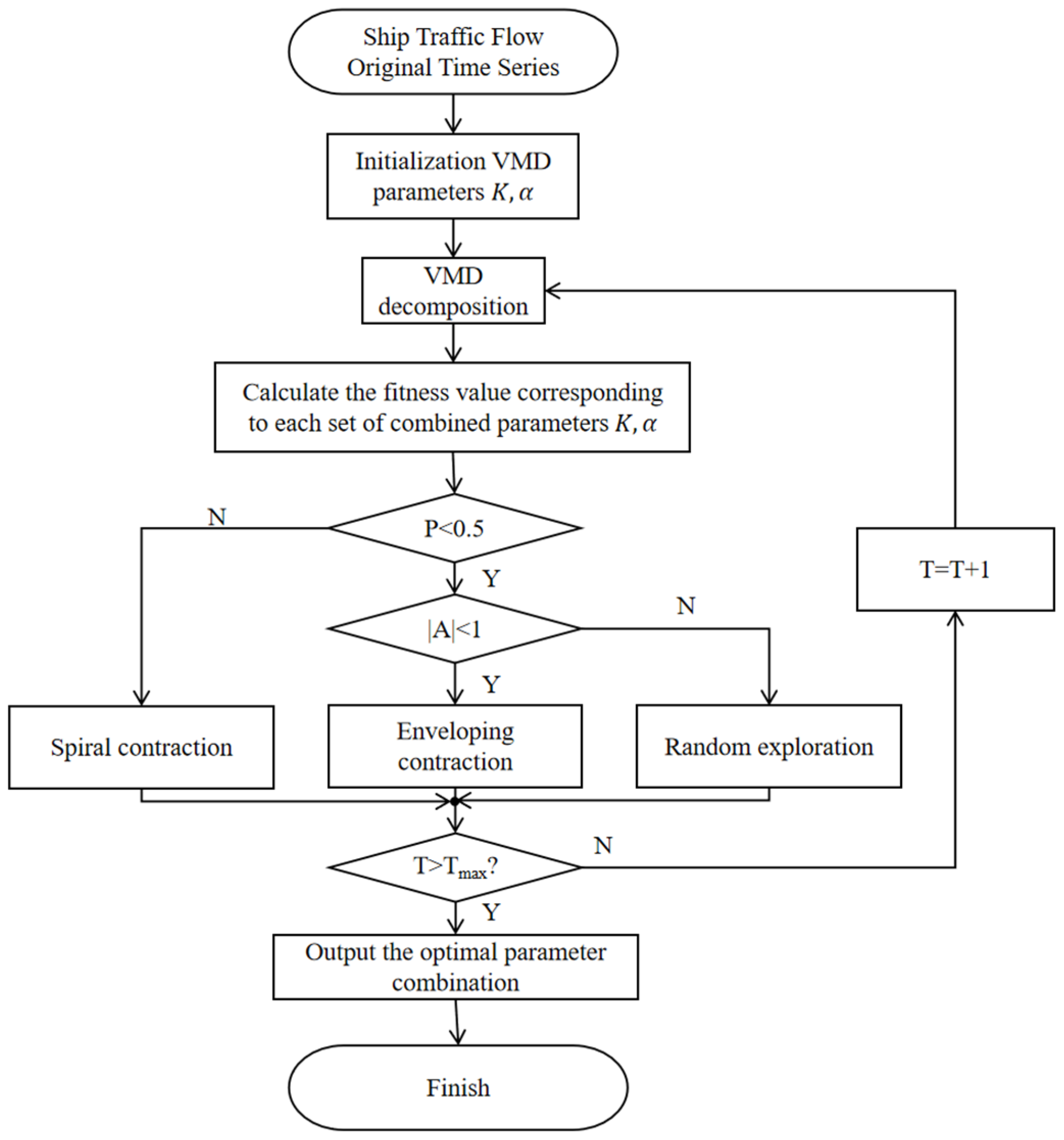
The decomposition performance of VMD largely depends on the appropriate selection of the mode number K and the penalty parameter α . However, manual or empirical parameter settings are often inefficient and prone to local optima. To address this issue, this study employs the Whale Optimization Algorithm (WOA) [32] to adaptively search for optimal parameters and establishes a WOA–VMD framework. The main procedure is as follows:
(1)
Initialization and fitness evaluation: The parameter ranges of K and α are initialized, and N individuals X i = ( K i , α i ) are randomly generated within the defined ranges. The maximum number of iterations T max is specified. For each individual, VMD is performed, and the mean squared reconstruction error (MSE) is adopted as the fitness function.
(2)
Position update mechanism:
① Encircling prey (local exploitation): The positions of candidate solutions are adjusted with respect to the current best solution, as defined in Equation (3).
D = C X * ( t ) X ( t ) X ( t + 1 ) = X * ( t ) A D
Here, X ( t ) denotes the position of the candidate solution at iteration t; D represents the difference between the current parameter set in each dimension ( K , α ) and the optimal combination; A and C are coefficient vectors, where A = 2 a r 1 a , C = 2 r 2 . During the iterations, the control parameter a decreases linearly from 2 to 0, while r 1 and r 2 are random vectors uniformly distributed in [0, 1]. This phase simulates the shrinking encirclement of whales around their prey to approximate the global optimum. When A < 1 , the algorithm emphasizes local exploitation by approaching the current best solution.
② Bubble-net attacking mechanism (spiral update): Whales perform bubble-net attacks by following a spiral trajectory, as formulated in Equation (4).
X ( t + 1 ) = D e b l cos ( 2 π l ) + X ( t ) D = X ( t ) X ( t )
Here, D denotes the distance between the current agent and the best agent; b is a constant that defines the logarithmic spiral shape; and l is a random number uniformly distributed in the interval [−1, 1].
③ Random search (global exploration phase): a random candidate solution X r a n d is introduced when A > 1 :
X ( t + 1 ) = X r a n d A | C X r a n d X ( t ) |
(3)
Stopping criterion: the optimal solution X * = ( K * , α * ) is returned when the maximum number of iterations is reached or a convergence criterion is met.
This optimization strategy effectively mitigates the subjectivity of manual parameter adjustment and the risk of being trapped in local optima by balancing local exploitation and global exploration. As a result, it enhances the robustness and objectivity of VMD in decomposing inland waterway traffic sequences. The flowchart is shown in Figure 2.

3.3. Pearson Correlation Coefficient (PCC)

To prevent over-decomposition of inland waterway traffic flow data by VMD and the resulting generation of redundant intrinsic components, the intrinsic mode functions (IMFs) obtained from the decomposition were quantitatively assessed using the Pearson correlation coefficient. Initially, the proportion of each IMF’s variance relative to the total variance of the reconstructed signal was calculated to evaluate its variance contribution. IMFs with variance contributions below a predefined threshold were identified as redundant. Subsequently, the linear correlation between each IMF and the original signal was measured using the Pearson correlation coefficient. The formula of the Pearson correlation coefficient is given in Equation (6) [33].
ρ x t , x I M F = cov ( x t , x I M F ) σ x t σ x I M F = E ( x t E ( x t ) ) ( x I M F E ( x I M F ) ) σ x t σ x I M F σ x t = E ( x t 2 ) E 2 ( x t ) σ x I M F = E ( x I M F 2 ) E 2 ( x I M F ) cov ( x t , x I M F ) = E ( x t , x I M F ) E ( x t ) E ( x I M F )
where ρ x t x I M F represents the global correlation coefficient, E ( ) denotes the expectation operator, cov ( x t , x I M F ) denotes the covariance between x t and x I M F , and the correlation coefficient r ( x t , x I M F ) is defined as:
r ( x t , x I M F ) = ( x t x t ¯ ) ( x I M F x I M F ¯ ) ( x t x t ¯ ) 2 ( x I M F x I M F ¯ ) 2
The classification of the correlation coefficient r ( x t , x I M F ) is presented in Table 1 [34].
The Pearson correlation coefficient (PCC) was employed to filter out weakly correlated information in order to reduce the computational burden of the predictive model, while intrinsic mode functions (IMFs) with stronger correlations were selected for signal reconstruction, thereby ensuring that the retained components preserve the representativeness of the original signal.

3.4. Multi-Head Attention Mechanism Integrated with LSTM

To fully leverage the features of IMF components extracted by VMD and filtered via Pearson correlation, a prediction module integrating multi-head attention (MHA) with long short-term memory (LSTM) is developed to better capture the nonlinear and temporal dependencies in ship traffic flow data. The main steps are outlined as follows:
(1)
Input layer: The IMFs are combined with auxiliary features such as geospatial coordinates (latitude, longitude and vessel speed), and others to form the input tensor X R B × T × F , where B denotes the batch size, T the time steps, and F the input feature dimension.
(2)
Multi-Head Attention Mechanism: To capture the global temporal dependencies across different time steps in ship traffic flow sequences, the multi-head attention mechanism is introduced to derive informative representations from the input sequence. Specifically, the sequence X is linearly projected into query (Q), key (K), and value (V) vectors. Attention weights are then computed to assign varying levels of importance to different features, thereby enhancing the model’s capacity to characterize nonlinear dynamics and multi-scale variations.
(3)
LSTM-based temporal modeling: The sequence features encoded by the attention mechanism are fed into the LSTM network to capture the temporal dependency and dynamic evolution patterns of ship traffic flow. The LSTM achieves dynamic memory and information updating through its gating structure, thereby effectively extracting the temporal evolution characteristics of the traffic sequence. Finally, the output layer of the LSTM predicts the ship traffic flow values at future time steps. The model employs a multi-head attention mechanism to enhance the global representation capability of the input features and an LSTM network to capture temporal dependencies, thereby achieving high-accuracy prediction of vessel traffic flow in high-traffic maritime areas under complex weather conditions.

4. Experimental Results and Analysis

In order to comprehensively evaluate the generalization capacity and adaptability of the proposed model in predicting vessel traffic flow within high-traffic inland waterway regions, three representative AIS datasets were selected, denoted as “Dataset A,” “Dataset B,” and “Dataset C.” These datasets are derived from the southern inland waterways, near-port corridors, and trunk channels of the United States, respectively. They encompass diverse geographical environments and traffic density conditions, thereby ensuring strong representativeness. All datasets used in this study were obtained from MarineCadastre.gov (https://hub.marinecadastre.gov/pages/vesseltraffic (accessed on 20 October 2024)), a maritime geospatial data-sharing platform provided by the U.S. government. The raw Automatic Identification System (AIS) trajectory data can be accessed online by specifying the temporal and spatial (latitude–longitude) range. For consistency, the sampling interval of each dataset was set to two hours, and each record contains the vessel’s MMSI, type, course, speed, length, beam, longitude, and latitude. A comparative summary is provided in Table 2.
During data preprocessing, records with apparent positional errors were removed, and those with zero or missing speed values were corrected using linear interpolation. Subsequently, all vessel reports were aggregated with a temporal resolution of 2 h to derive statistical features such as the number of vessels (MMSI count), the average speed, and the centroid coordinates (latitude and longitude) at each time step. To ensure temporal consistency and spatial comparability across different regions, temporal alignment and feature normalization were performed on all variables. Subsequently, input–output samples were constructed using a sliding-window approach for model training [35].
In time series analysis, the standard deviation of the first-order differences is commonly employed to quantify the volatility of a sequence. A larger value indicates stronger short-term fluctuations, reflecting higher complexity and instability [36]. Therefore, in this study, the standard deviation of differenced traffic flow series is utilized as an auxiliary metric to capture the intensity of nonlinearity under complex canal environments. As shown in Figure 3, the volatility is markedly higher at lock locations or under adverse meteorological conditions, implying that traffic flow nonlinearity becomes more pronounced in such scenarios.
To ensure sufficient model training and objective evaluation, the dataset was partitioned into 85% for training and 15% for testing. All experiments were implemented using PyTorch 1.13.0 and Python 3.7.13, with PyCharm IDE version 2021.3 as the development environment. The computational platform consisted of an Intel® Core™ i5-8600K CPU @ 3.6 GHz (Intel Corporation, Santa Clara, CA, USA), an NVIDIA GeForce RTX 2080 Ti GPU (NVIDIA Corporation, Santa Clara, CA, USA), and 16 GB RAM.

4.1. Experimental Evaluation Index

To comprehensively evaluate the performance of the proposed model in vessel traffic flow prediction, the mean squared error (MSE), root mean squared error (RMSE), and coefficient of determination (R2) are employed to quantitatively assess its predictive capability. These metrics characterize the deviation between predicted and observed values from complementary perspectives, including error magnitude, variability, relative deviation, and goodness-of-fit, with their formal definitions given as follows:
(1)
Mean Squared Error (MSE) is defined as the mean of the squared residuals between predicted and actual values, quantifying the overall deviation of predictions from observations, as formally expressed in Equation (8).
M S E = 1 n i = 1 n ( y i y i ^ ) 2
(2)
Root Mean Squared Error (RMSE) measures the standard deviation of the residuals, with smaller values indicating higher predictive accuracy, as defined in Equation (9).
R M S E = 1 n i = 1 n ( y i y i ^ ) 2
(3)
The coefficient of determination (R2) is a statistical metric that evaluates the goodness-of-fit of the model by indicating the proportion of variance in the observed data explained by the predictions.
R 2 = 1 i = 1 n ( y i y i ^ ) 2 i = 1 n ( y i y ¯ ) 2
where y i denotes the observed data, y ^ i denotes the predicted value, y ¯ represents the mean of the ground truth values, and n is the sample size. In this study, the LSTM architecture is configured as a 2-layer model with 128 hidden units per layer, while the remaining hyperparameters are specified in Table 3.

4.2. WOA-VMD Parameter Selection

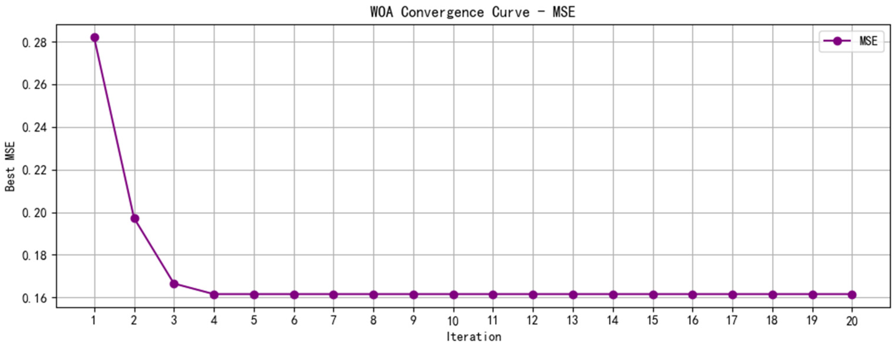
The WOA-optimized VMD (WOA-VMD) model is validated using dataset A, which is sampled at a 2-h interval. The dataset is decomposed into intrinsic mode functions (IMFs), and the corresponding correlation coefficient weight matrix is obtained. The optimal decomposition results are achieved by optimizing the number of modes (K) in VMD through the Whale Optimization Algorithm (WOA), with the hyperparameter settings listed in Table 4. Figure 4 illustrates the convergence curve of the optimization process, where the mean squared error (MSE) is employed as the fitness function. It can be observed that the MSE converges to its optimal value of 0.164 at the 4th iteration.
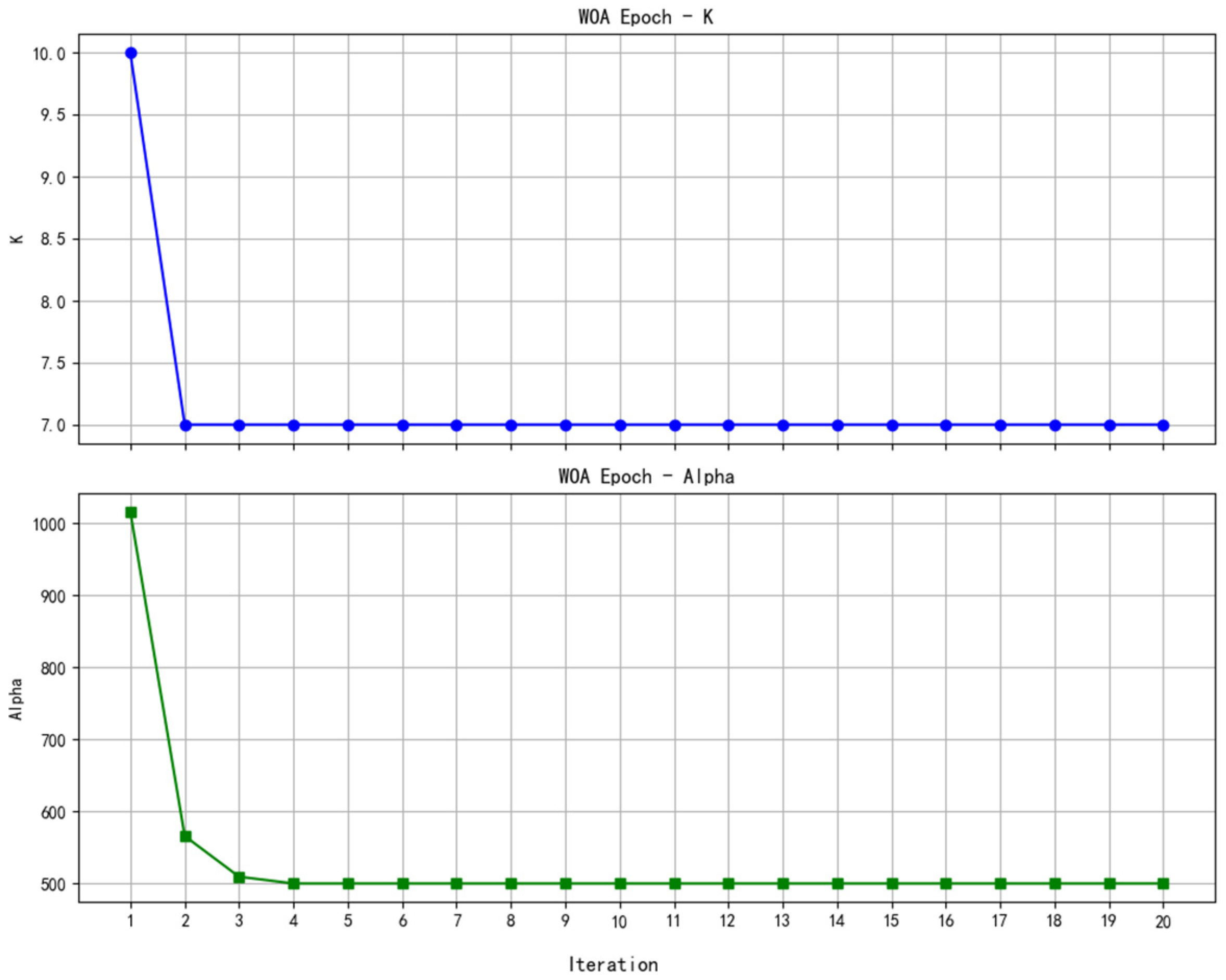
During the parameter optimization of Variational Mode Decomposition (VMD) via the Whale Optimization Algorithm (WOA), the algorithm converges to the optimal solution within 20 iterations. Figure 5 illustrates the convergence trajectories of the parameters, which ultimately stabilize at 7 and 500, corresponding to the optimal parameter settings for the VMD.
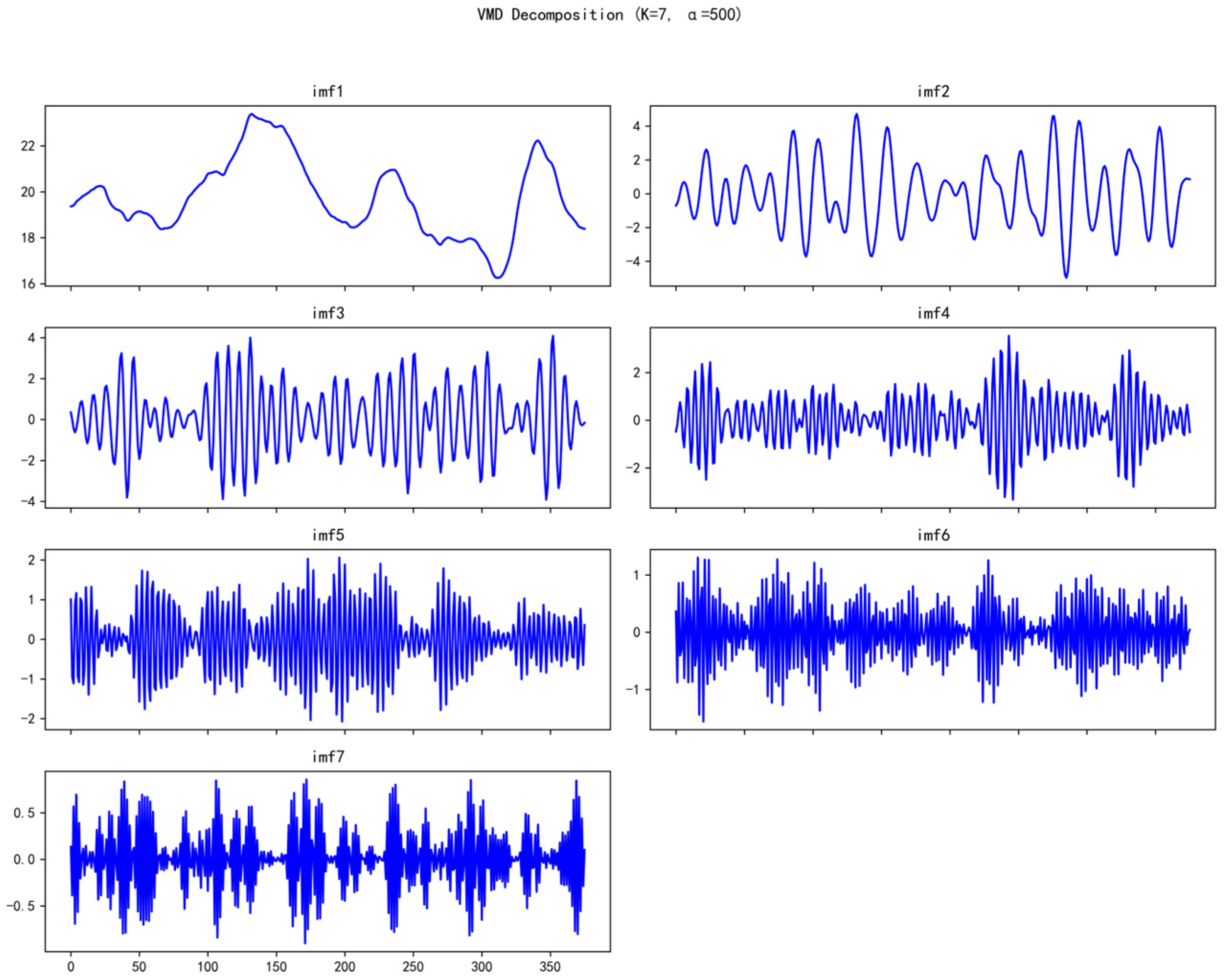
The optimal parameters of Variational Mode Decomposition (VMD)—namely, the number of modes ( K ) and the penalty factor ( α )—were identified by the Whale Optimization Algorithm (WOA) within 20 iterations. Based on this parameter configuration, the ship traffic flow data sampled at a 2-h interval were decomposed to obtain several intrinsic mode functions (IMFs). Figure 6 illustrates the IMFs derived from the VMD results. As shown in the figure, IMF1 and IMF2 correspond to low-frequency components, primarily capturing the long-term trends in AIS-based vessel traffic flow data. IMF1 exhibits relatively smooth variations, characterized by a pronounced global trend. The intermediate components, IMF3–IMF5, correspond to mid-frequency modes, capturing the periodic oscillations of vessel traffic flow, potentially associated with traffic peak periods. These components are often the most informative, as they represent the primary dynamic characteristics of vessel traffic. By contrast, IMF7 corresponds to a high-frequency component, which may indicate sudden perturbations, typically manifested as noise.
In this experiment, Intrinsic Mode Functions (IMFs) with a Pearson correlation coefficient exceeding 0.2 were retained for signal reconstruction. This approach mitigates model complexity while suppressing noise, without discarding an excessive number of IMFs and thereby preventing substantial deviation between the reconstructed and original signals.
The Pearson correlation coefficients of IMF1 through IMF6 exceed 0.2, while the high-frequency component IMF7 was discarded. The signal was reconstructed using IMF1–IMF6, yielding a mean squared error (MSE) of 0.3753 between the reconstructed and original signals, with a coefficient of determination (R2) of 0.9764. The Pearson correlation coefficients of the IMFs relative to the original signal are presented in Table 5 and Figure 7.

4.3. WVMA-LSTM Model Prediction Results

4.3.1. Optimization Contrast Experiment

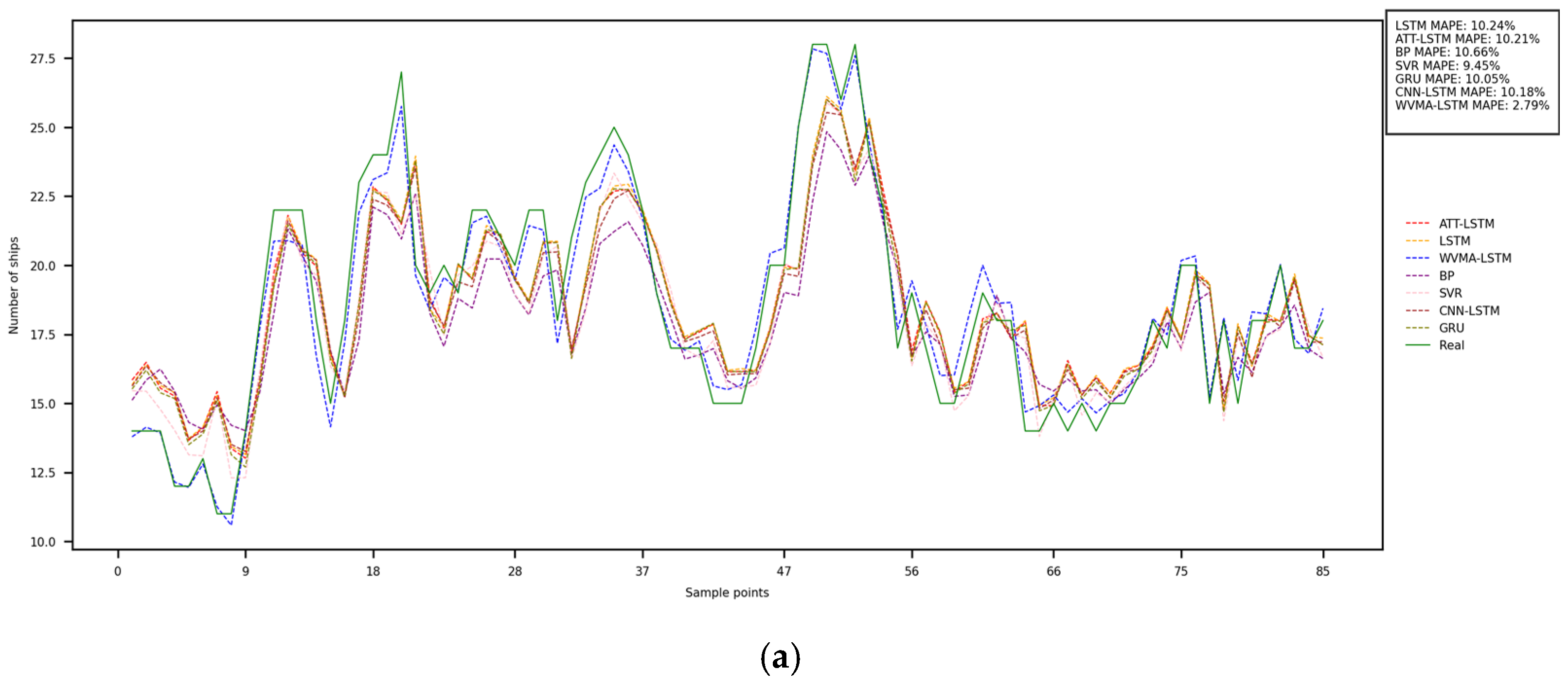
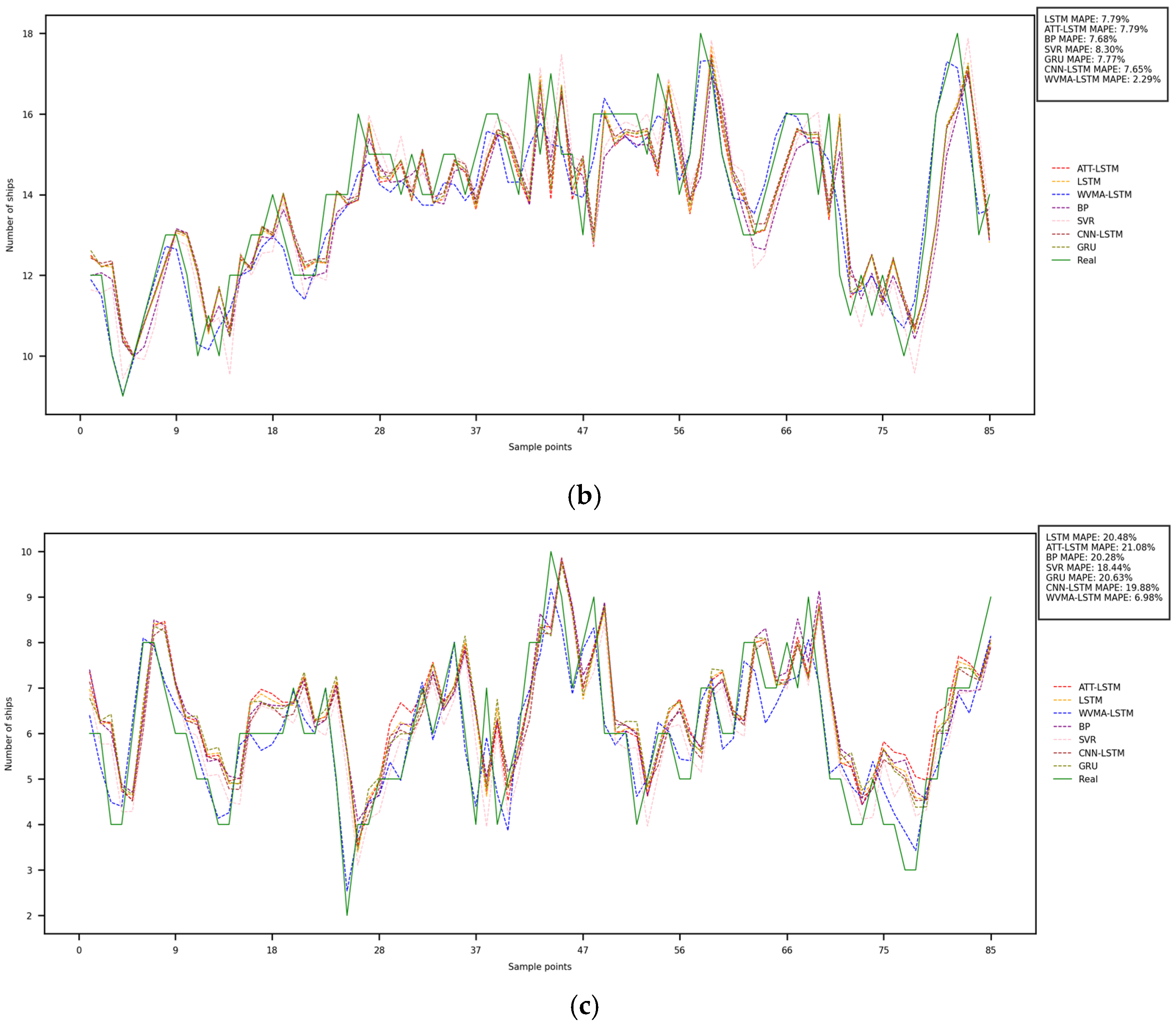
To validate the effectiveness of the proposed WVMA-LSTM model in predicting vessel passage through canal locks, and to assess its robustness under adverse weather conditions (e.g., rainfall and strong winds), we employ regional datasets sampled at 2-h intervals. Model performance is evaluated using MSE, RMSE, and R2 metrics. Table 6 presents a comparative analysis between the WVMA-LSTM and several baseline models, including the standard LSTM, ATT-LSTM, BP neural network, gated recurrent unit (GRU), CNN-LSTM, and Support Vector Regression (SVR).
Table 6 and Figure 8 indicate that under varying traffic density conditions, the prediction accuracy of different models differs significantly. Traditional approaches such as BP, SVR, and standalone LSTM or GRU models exhibit some predictive capability in high-traffic regions under adverse weather, but their overall accuracy remains limited. In the Dataset C test set (20–26 June 2024), vessel traffic flow in the study area was strongly influenced by the operation of the Desen Island and Marses Locks, leading to pronounced fluctuations. During this period, the R2 of conventional LSTM and GRU models remained below 40%, while even the comparatively better-performing SVR achieved only 41.73%, indicating their inability to effectively capture the complex nonlinear dynamics. Similarly, in the Dataset B test set (29 May–4 June 2024), during periods influenced by port operations and tidal disturbances, the prediction accuracies of conventional methods remain below 60% and exhibit a pronounced lag in responding to abrupt traffic flow variations. This finding indicates that existing methods fail to address the challenges highlighted in this study when confronted with highly nonlinear and complex scenarios. By contrast, the WVMA-LSTM model demonstrates clear superiority under the same conditions. Within these challenging intervals, the WVMA-LSTM model achieves R2 values of 89.88% and 90.82% on Datasets B and C, substantially outperforming the baseline models and yielding markedly lower MSE and RMSE values. This demonstrates that the adaptive adjustment of VMD parameters via the Whale Optimization Algorithm effectively mitigates the non-stationarity and nonlinearity of traffic sequences, while enhancing the attention mechanism’s capability to extract multimodal features, thereby enabling the model to accurately capture abrupt traffic flow variations under adverse weather conditions and in high-density traffic regions. WVMA-LSTM not only substantially enhances overall prediction accuracy, but more importantly, it effectively addresses the core challenge identified in this study during nonlinear, strongly perturbed intervals where traditional models fail.

4.3.2. Ablation Experiment

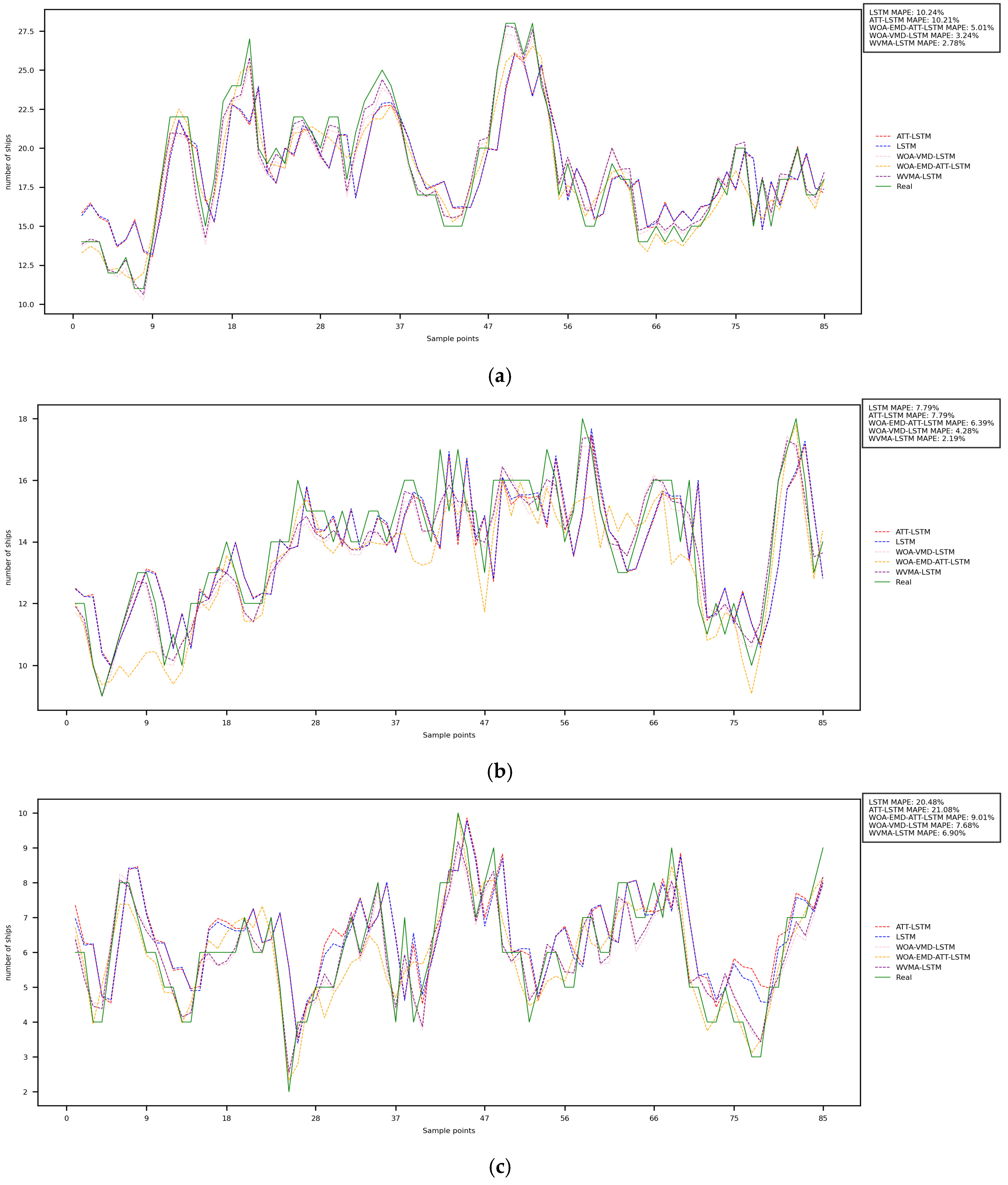
Ablation experiments were conducted to evaluate the effectiveness of each component of the WVMA-LSTM model, as illustrated in Figure 9. The results for a 2-h prediction horizon are summarized in Table 7, where the WOA-EMD-ATT-LSTM is denoted as WEA-LSTM and the WOA-VMD-LSTM is denoted as WV-LSTM.
Table 7 shows that the R2 values of the baseline LSTM model and the ATT-LSTM are generally below 70% across the three datasets and drop to around 30% in dataset C. This result reveals their limited capacity to capture nonlinear characteristics in complex inland waterway environments. The WOA-EMD-LSTM model, augmented with the Whale Optimization Algorithm (WOA), demonstrates substantial improvement on datasets A and C, achieving R2 values of 91.35% and 83.19%, respectively. This suggests that WOA effectively alleviates parameter optimization challenges and enhances model stability. However, due to the inherent mode mixing issue in EMD, the overall predictive accuracy remains suboptimal, and the model is still inadequate in fully capturing the nonlinear dynamics of vessel traffic flow in inland waterway scenarios. In contrast, the WOA-VMD-LSTM significantly outperforms the WOA-EMD-LSTM across all three datasets, indicating that VMD is more effective in mitigating the non-stationary and nonlinear characteristics of vessel traffic flow sequences. Ultimately, the WVMA-LSTM, by integrating the strengths of VMD and the multi-head attention mechanism, achieves the best predictive performance across all datasets, thereby demonstrating both the effectiveness and robustness of the proposed approach in complex inland waterway traffic environments.
More importantly, the improvement in prediction accuracy is not only statistically significant but also operationally meaningful. Under high-traffic and complex scheduling scenarios, accurate flow prediction provides decision-support information for vessel scheduling optimization, assisting port and lock authorities in optimizing passage windows to mitigate congestion and reduce dwell times. Moreover, it enables dynamic traffic management and risk prediction by identifying potential bottlenecks or overloaded zones in advance, thereby enhancing navigational efficiency and safety. Particularly in inland waterway hub regions with frequent meteorological disturbances or high vessel density, the highly accurate forecasts produced by the WVMA-LSTM model can directly support the real-time optimization of intelligent dispatching and traffic management platforms, playing a crucial role in improving navigational safety and enhancing channel capacity.

5. Conclusions and Future Directions

To address the challenge of predicting vessel traffic in high-density regions of inland waterways under complex environmental conditions, where strong nonlinearity considerably increases prediction difficulty, a WVMA-LSTM model is proposed. By integrating Variational Mode Decomposition (VMD), a multi-head attention mechanism, and LSTM, the model effectively mitigates the issues of non-stationarity and multi-scale characteristics in vessel traffic flow time series. Furthermore, the VMD parameters are adaptively optimized using the Whale Optimization Algorithm (WOA), thereby enhancing the decomposition performance and overall predictive accuracy. Finally, the WVMA-LSTM model is developed to establish a complete optimization–decomposition–prediction framework, thereby enhancing the accuracy and robustness of vessel traffic flow prediction in inland canal scenarios. The experimental results demonstrate that under varying traffic conditions and adverse weather influences, the WVMA-LSTM model achieves a higher and more stable goodness of fit compared with both a baseline model without decomposition and a model incorporating EMD-based decomposition. This indicates that the proposed model can mitigate data nonlinearity by decomposing vessel traffic flow data in inland canal scenarios, thereby extracting multi-scale representations and enriching the feature space, which ultimately enhances prediction accuracy.
The choice of WOA is primarily motivated by its simple structure, rapid convergence, minimal parameter tuning requirements, and robust global exploration capability, which make it particularly suitable for addressing highly nonlinear and multimodal optimization problems in VMD parameter tuning. It should be noted that the Whale Optimization Algorithm (WOA) adopted in this study represents only one instance within the broader class of evolutionary algorithms. Future work could explore the incorporation of other evolutionary optimization algorithms, such as Genetic Algorithms (GAs) and Particle Swarm Optimization (PSO), into the VMD-LSTM framework to evaluate their comparative performance with respect to convergence rate, global exploration capability, and predictive accuracy. Considering the advantage of Genetic Algorithms (Gas) in maintaining population diversity and the superior convergence efficiency of Particle Swarm Optimization (PSO) in continuous optimization problems, incorporating these alternative algorithms can further assess the generalizability of the “optimize–decompose–predict” framework and provide more robust evolutionary-based optimization strategies for ship traffic flow prediction in complex environments. Although the proposed model demonstrates strong capability in handling nonlinear time series, it still has several limitations. Firstly, as the model simultaneously integrates VMD, a multi-head attention mechanism, and a two-layer LSTM architecture, its overall computational complexity is relatively high. This results in greater demands on hardware resources, posing challenges for real-time deployment. Secondly, the model is sensitive to the quality of input data; in particular, inaccuracies in environmental features such as meteorological and tidal information can substantially degrade prediction performance. In addition, the applicability of the model to specific waterways or port areas remains to be further validated.

Author Contributions

Conceptualization, L.L. and M.W.; software, L.L.; experiment analysis, L.L., X.S. and L.F.; writing—review and editing, L.L., M.W., C.Q. and R.K.; funding acquisition, M.W. and C.Q.; investigation, L.L.; visualization, L.L.; supervision, L.L. and M.W.; project administration, L.L., M.W. and C.Q. All authors have read and agreed to the published version of the manuscript.

Funding

This research is funded by the Guangxi Science and Technology Major Program under Grant No. GuikeAA23062035 and Grant No. GuikeAD23026032. This work is also supported by the National Natural Science Foundation of China under Grant 62101293.

Institutional Review Board Statement

Not applicable.

Informed Consent Statement

Not applicable.

Data Availability Statement

We are unreservedly willing to provide research data or key codes mentioned in this manuscript. If necessary, please contact Liu-Lu Luo via email (2120231214@glut.edu.cn) to obtain the Baidu Netdisk (Baidu Cloud) URL link and then download the files you need.

Acknowledgments

We are all very grateful to the volunteers and staff from GLUT and GUET for their selfless assistance during our experiments.

Conflicts of Interest

The authors declare no conflicts of interest.

References

  1. Baldauf, M.; Fischer, S.; Kitada, M.; Mehdi, R.; Al-Quhali, M.; Fiorini, M. Merging conventionally navigating ships and MASS—Merging VTS, FOC and SCC. TransNav Int. J. Mar. Navig. Saf. Sea Transp. 2019, 13, 495–501. [Google Scholar] [CrossRef]
  2. Praetorius, G. Vessel Traffic Service (VTS): A Maritime Information Service or Traffic Control System: Understanding Everyday Performance and Resilience in a Socio-Technical System under Change. Ph.D. Thesis, Chalmers Tekniska Högskola, Gothenburg, Sweden, 2014. [Google Scholar]
  3. Relling, T.; Praetorius, G.; Hareide, O.S. A socio-technical perspective on the future Vessel Traffic Services. Necesse 2019, 4, 112–129. [Google Scholar]
  4. Cho, K.; Van Merrienboer, B.; Gulcehre, C.; Bahdanau, D.; Bougares, F.; Schwenk, H.; Bengio, Y. Learning phrase representations using RNN encoder–decoder for statistical machine translation. arXiv 2014, arXiv:1406.1078. [Google Scholar]
  5. Xu, X.; Bai, X.; Xiao, Y.; Sun, X.; Xu, Z. A port ship flow prediction model based on the automatic identification system and gated recurrent units. J. Mar. Sci. Appl. 2021, 20, 572–580. [Google Scholar] [CrossRef]
  6. Chung, J.; Gulcehre, C.; Cho, K.H.; Bengio, Y. Empirical evaluation of gated recurrent neural networks on sequence modeling. arXiv 2014, arXiv:1412.3555. [Google Scholar] [CrossRef]
  7. Wang, Y.B.; Papageorgiou, M. Real-time freeway traffic state estimation based on extended Kalman filter: A general approach. Transp. Res. Part B Methodol. 2005, 39, 141–167. [Google Scholar] [CrossRef]
  8. Box, G.E.P.; Jenkins, G.M.; Reinsel, G.C. Time Series Analysis: Forecasting and Control. J. Oper. Res. Soc. 1976, 22, 199–201. [Google Scholar]
  9. He, W.; Zhong, C.; Sotelo, M.A.; Chen, H.; Zhao, D. Short-term vessel traffic flow forecasting by using an improved Kalman model. Clust. Comput. 2019, 22, 7907–7916. [Google Scholar] [CrossRef]
  10. Zhao, W.; Gao, Y.; Ji, T.; Chen, L.; Zhang, Y. Deep temporal convolutional networks for short-term traffic flow forecasting. IEEE Access 2019, 7, 114496–114507. [Google Scholar] [CrossRef]
  11. Man, J.; Chen, D.; Wu, B.; Wan, C.P.; Yan, X.P. An effective approach for Yangtze River vessel traffic flow forecasting: A case study of Wuhan area. Ocean Eng. 2024, 296, 116899. [Google Scholar] [CrossRef]
  12. Lee, T.-L. Back-propagation neural network for the prediction of the short-term storm surge in Taichung Harbor, Taiwan. Eng. Appl. Artif. Intell. 2008, 21, 63–72. [Google Scholar] [CrossRef]
  13. Wang, X.; Li, J.; Zhang, T. A machine-learning model for zonal ship flow prediction using AIS data: A case study in the South Atlantic States region. J. Mar. Sci. Eng. 2019, 7, 463. [Google Scholar] [CrossRef]
  14. Ma, X.; Tao, Z.; Wang, Y.; Yu, H.; Wang, Y. Long short-term memory neural network for traffic speed prediction using remote microwave sensor data. Transp. Res. Part C Emerg. Technol. 2015, 54, 187–197. [Google Scholar] [CrossRef]
  15. Chen, S.; Lin, C.; Gu, Y.; Sheng, J.; Hariri-Ardebili, M.A. Dam deformation data preprocessing with optimized variational mode decomposition and kernel density estimation. Remote Sens. 2025, 17, 718. [Google Scholar] [CrossRef]
  16. Zhang, Z.G.; Yin, J.C.; Wang, N.N.; Liu, H.; Li, X. Vessel traffic flow analysis and prediction by an improved PSO-BP mechanism based on AIS data. Evol. Syst. 2019, 10, 397–407. [Google Scholar] [CrossRef]
  17. Lu, W.; Dong, B.; Wang, Z. Short-term traffic flow prediction based on CNN–SVR hybrid deep learning model. J. Transp. Syst. Eng. Inf. Technol. 2017, 17, 68–74. (In Chinese) [Google Scholar]
  18. Cai, L.; Lei, M.; Zhang, S.; Yu, Y.; Zhou, T.; Qin, J. A noise-immune LSTM network for short-term traffic flow forecasting. Chaos Interdiscip. J. Nonlinear Sci. 2020, 30, 023135. [Google Scholar] [CrossRef] [PubMed]
  19. Muthukumaran, V.; Natarajan, R.; Kaladevi, A.C.; Devi, M.; Sharma, R. Traffic flow prediction in inland waterways of Assam region using uncertain spatiotemporal correlative features. Acta Geophys. 2022, 70, 2979–2990. [Google Scholar] [CrossRef]
  20. Zhuang, W.; Cao, Y. Short-term traffic flow prediction based on a K-nearest neighbor and bidirectional long short-term memory model. Appl. Sci. 2023, 13, 2681. [Google Scholar] [CrossRef]
  21. Dong, Z.; Zhou, Y.; Bao, X. A short-term vessel traffic flow prediction based on a DBO-LSTM model. Sustainability 2024, 16, 5499. [Google Scholar] [CrossRef]
  22. Xiang, Z.; Yan, J.; Demir, I. A rainfall–runoff model with LSTM-based sequence-to-sequence learning. Water Resour. Res. 2020, 56, e2019WR025326. [Google Scholar] [CrossRef]
  23. Kao, I.F.; Zhou, Y.; Chang, L.C.; Chang, F.J. Exploring a long short-term memory-based encoder–decoder framework for multi-step-ahead flood forecasting. J. Hydrol. 2020, 583, 124596. [Google Scholar] [CrossRef]
  24. Akopov, A.S.; Beklaryan, L.A. Evolutionary synthesis of high-capacity reconfigurable multilayer road networks using a multiagent hybrid clustering-assisted genetic algorithm. IEEE Access 2025, 13, 53448–53474. [Google Scholar] [CrossRef]
  25. Tseng, Y.-T.; Ferng, H.-W. An improved traffic rerouting strategy using real-time traffic information and decisive weights. IEEE Trans. Veh. Technol. 2021, 70, 9741–9751. [Google Scholar] [CrossRef]
  26. Xiao, H.; Zhao, Y.; Zhang, H. Predict vessel traffic with weather conditions based on multimodal deep learning. J. Mar. Sci. Eng. 2023, 11, 39. [Google Scholar] [CrossRef]
  27. Zhang, Y.; Li, X.; Wang, H. Integrated optimization of lock scheduling and vessel traffic flow under adverse weather. Transp. Res. Part C Emerg. Technol. 2023, 147, 105789. [Google Scholar]
  28. Pavlyuk, D. Spatiotemporal cross-validation of urban traffic forecasting models. Transp. Res. Procedia 2021, 52, 179–186. [Google Scholar] [CrossRef]
  29. Gao, R.; Du, L.; Suganthan, P.N.; Zhou, Q.; Yuen, K.F. Random vector functional link neural network-based ensemble deep learning for short-term load forecasting. Expert Syst. Appl. 2022, 206, 117784. [Google Scholar] [CrossRef]
  30. Zhang, J.; Xin, X.; Shang, Y.; Wang, Y.; Zhang, L. Nonstationary significant wave height forecasting with a hybrid VMD–CNN model. Ocean Eng. 2023, 285, 115338. [Google Scholar] [CrossRef]
  31. Ouyang, M.; Shen, P. Prediction of remaining useful life of lithium batteries based on WOA–VMD and LSTM. Energies 2022, 15, 8918. [Google Scholar] [CrossRef]
  32. Dragomiretskiy, K.; Zosso, D. Variational mode decomposition. IEEE Trans. Signal Process. 2014, 62, 531–544. [Google Scholar] [CrossRef]
  33. Yin, G. Research on Useful Life Prediction of Rolling Bearing Based on Pearson-KPCA Multi-Feature Fusion. Master’s Thesis, Harbin University of Science and Technology, Harbin, China, 2021. [Google Scholar]
  34. Mirjalili, S.; Lewis, A. The whale optimization algorithm. Adv. Eng. Softw. 2016, 95, 51–67. [Google Scholar] [CrossRef]
  35. Hochreiter, S.; Schmidhuber, J. Long short-term memory. Neural Comput. 1997, 9, 1735–1780. [Google Scholar] [CrossRef] [PubMed]
  36. Engle, R.F. Autoregressive conditional heteroscedasticity with estimates of the variance of United Kingdom inflation. Econometrica 1982, 50, 987–1007. [Google Scholar] [CrossRef]
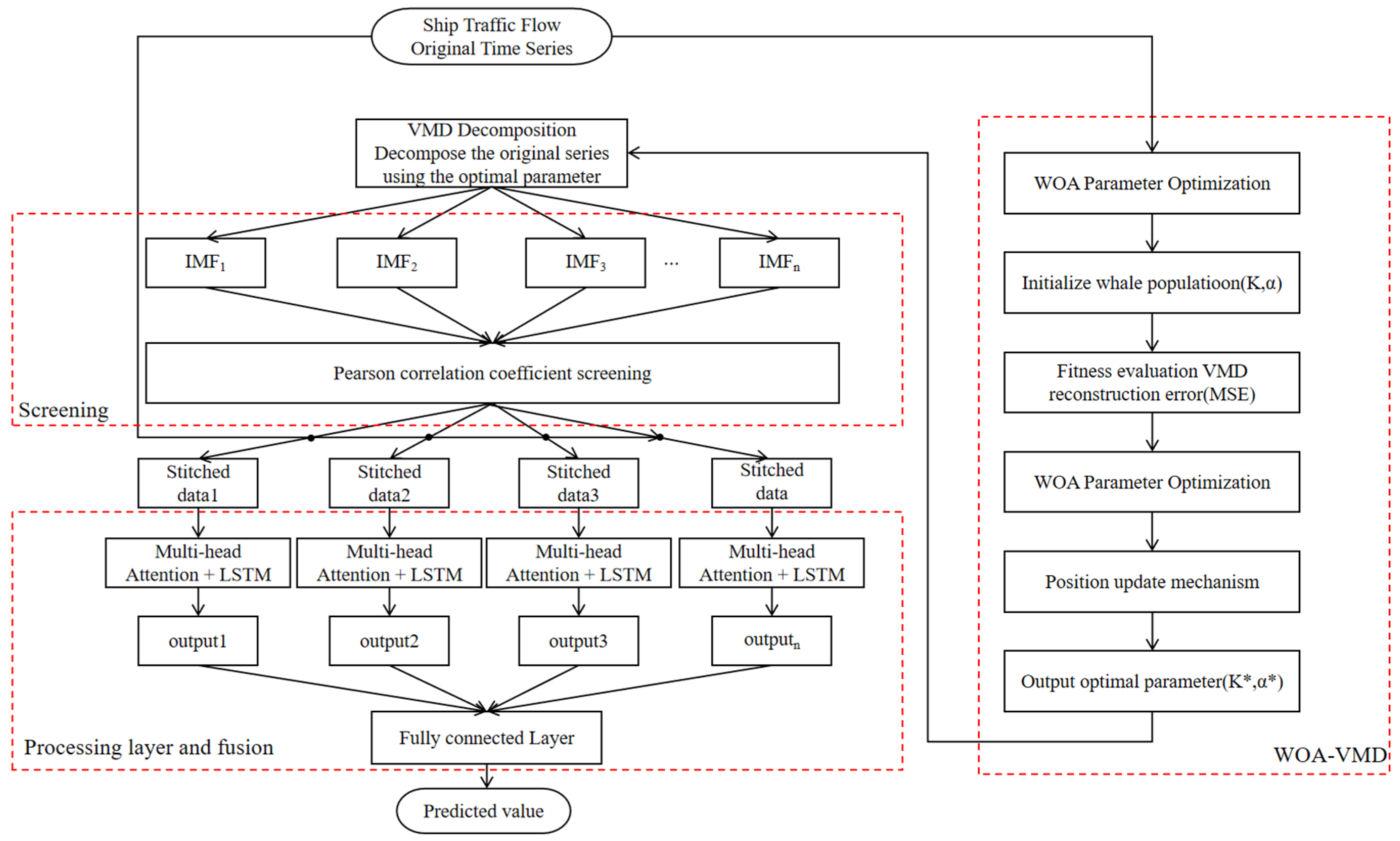
Figure 1. WVMA-LSTM Model. The asterisk denotes the optimal value.
Applsci 15 11776 g001
Figure 2. Whale Optimization Algorithm for VMD Parameter Optimization.
Applsci 15 11776 g002
Figure 3. Comparison of standard deviation of traffic flow variance of each dataset in lockout and bad weather.
Applsci 15 11776 g003
Figure 4. Iteration curve of fitness function MSE.
Applsci 15 11776 g004
Figure 5. The parameter K of VMD and the iterative curve optimized by WOA.
Applsci 15 11776 g005
Figure 6. IMF after decomposition of VMD with optimal parameter combination.
Applsci 15 11776 g006
Figure 7. The original signal and the Pearson coefficient correlation heat map of IMF.
Applsci 15 11776 g007
Figure 8. The prediction results of different models at 2 h time interval; (a) is Dataset A, (b) is Dataset B, (c) is Dataset C.
Applsci 15 11776 g008aApplsci 15 11776 g008b
Figure 9. Ablation experiment with a time interval of 2 h; (a) is Dataset A, (b) is Dataset B, (c) is Dataset C.
Applsci 15 11776 g009
Table 1. Classification of Pearson Correlation Coefficients.
Interrelation r ( x t , x I M F ) Coefficient Values
Very weakly correlated or uncorrelated0.0–0.2
Weakly correlated0.2–0.4
Moderate correlated0.4–0.6
Strongly related0.6–0.8
Extremely strong correlation0.8–1.0
Table 2. Dataset comparison and description.
DatasetTimeChannel CharacteristicsWeather Conditions
Dataset A4 April–21 May 2021Inland river freight corridor.5/16–19 Thunderstorm + gale
5/17 Extreme rainfall days
15–17 Overall weather is changeable.
Dataset B19 April–4 June 2021Affected by port dispatching and tidal changes, traffic fluctuates greatly.5/21–21 Mid to heavy rain
6/4 High wind
Dataset C11 May–26 June 2021It includes the Desen Island Lock and the Marces Lock, where traffic flow exhibits pronounced fluctuations and the navigational conditions are highly complex.6/20–21 Severe storm
6/21–26 Heavy rain and tornadoes
Table 3. Experimental parameters.
Parameter NameParameter SettingParameter NameParameter Setting
Number of trainings100OptimizerAdam
Learning rate1 × 10−3Dropout rate0.2
Input step size5Batch size32
Output step length1Loss functionMSE
Table 4. Whale optimization parameter setting value.
Parameter NameParameter Value
Number of whales10
Number of iterations20
Number of variables2
IMF scope[3, 15]
Scope[500, 5000]
Table 5. Pearson correlation coefficients of IMFs.
Modal ComponentCorrelation CoefficientModal ComponentCorrelation Coefficient
IMF10.5126IMF50.2812
IMF20.6235IMF60.2042
IMF30.5338IMF70.1495
IMF40.3679
Table 6. Performance comparison between the proposed model and baseline models in vessel traffic flow prediction at a 2-h interval.
DatasetDataset ADataset BDataset C
Evaluating IndicatorMSERMSER2 (%)MSERMSER2 (%)MSERMSER2 (%)
ATT-LSTM3.1061.26068.6371.8821.37256.5371.6811.29731.620
LSTM3.1051.25668.6441.8551.35357.1581.6011.26534.899
BP4.1021.47062.5251.8291.35357.7531.5821.25835.899
SVR2.8321.19870.3212.0351.42653.0091.4331.19741.731
CNN-LSTM1.1841.27768.1621.7531.32459.5151.5521.24636.881
GRU3.0821.25468.7871.8271.35257.8011.6361.27933.464
WVMA-LSTM0.3770.61493.6820.4380.66289.8760.2261.47590.822
Table 7. Comparison of evaluation indexes of ablation experiments with a time interval of 2 h.
DatasetDataset ADataset BDataset C
Evaluating IndicatorMSERMSER2 (%)MSERMSER2 (%)MSERMSER2 (%)
ATT-LSTM3.1061.26068.6371.8821.37256.5371.6811.29731.620
LSTM3.1051.25668.6441.8551.35357.1581.6011.26534.899
WEA-LSTM1.1091.18791.3471.3541.16468.7230.4130.64383.620
WV-LSTM0.5890.75492.5070.5330.73183.6870.2910.53988.181
WVMA-LSTM0.3670.60693.7430.4380.66289.8760.2210.47091.019
Disclaimer/Publisher’s Note: The statements, opinions and data contained in all publications are solely those of the individual author(s) and contributor(s) and not of MDPI and/or the editor(s). MDPI and/or the editor(s) disclaim responsibility for any injury to people or property resulting from any ideas, methods, instructions or products referred to in the content.