Article

A Loss Model System for Two-Dimensional Compressor Cascades of Modern Controlled Diffusion Airfoils

1
Research Institute of Aero-Engine, Beihang University, Beijing 100191, China
2
National Key Laboratory of Science and Technology on Aero-Engine Aero-Thermodynamics, Beihang University, Beijing 100191, China
3
School of Energy and Power Engineering, Beihang University, Beijing 100191, China
*
Author to whom correspondence should be addressed.
Appl. Sci. 2025, 15(21), 11759; https://doi.org/10.3390/app152111759
Submission received: 10 October 2025 / Revised: 31 October 2025 / Accepted: 3 November 2025 / Published: 4 November 2025

Abstract

The early design stage of modern compressors urgently requires high-accuracy, low-cost two-dimensional (2D) cascade loss prediction models. However, existing traditional loss models, predominantly based on early profile data, struggle to accurately predict the performance of modern Controlled Diffusion Airfoils (CDA). This study develops a comprehensive loss model system specifically for 2D cascades with modern CDA profiles. A numerical simulation database, encompassing the entire operating range of various subsonic, transonic, and supersonic profile designs, was first constructed to provide the data foundation for the model system development. Eight critical sub-models essential for the system were then identified based on an analysis of loss sources (including blade surface boundary layers and shock waves). A methodology combining physical mechanism analysis and data-driven techniques was applied to determine the final modeling scheme for each sub-model. Validation results demonstrate that within the parameter space covered by the database, the new model system achieves over 70% higher prediction accuracy compared to the traditional model system, with approximately 95% of prediction errors falling within ±0.02. It also accurately captures the variation trend of loss with incidence angle. The entire model system, consisting of a series of explicit formulas with clear physical meanings, can be easily integrated into compressor design processes and effectively support the design and analysis of airfoils during the preliminary stages of compressor development.

1. Introduction

The loss model for 2D cascades serves as one of the core tools for performance prediction during the preliminary design stages of compressors [1]. In recent years, blade profile design methodologies have advanced rapidly, and the design space has been significantly broadened. The CDA profiles, which manage boundary layer development through shape optimization [2], have been widely applied. Their superior performance has been confirmed by various studies [3,4,5]. However, the high design freedom of CDA profiles increases flow field complexity, greatly constraining the accuracy and generalizability of existing 2D cascade loss models. Therefore, developing a suitable loss prediction model for 2D cascades with modern CDA profiles is of great importance for improving the efficiency and reliability of preliminary compressor design.
Traditional 2D cascade loss models were generally constructed using early profile types. Lieblein [6] constructed a classic profile loss model based on extensive low-speed experimental data for NACA65, C4, and circular arcs profiles. Koch and Smith [7] as well as Aungier et al. [8] subsequently further modified this model to cover a wider range of profiles and Mach numbers. Miller et al. [9], Koch and Smith [7], Boyer and O’Brien [10], Wright and Miller [11], Sun et al. [12], and Banjac et al. [13] developed various shock loss models by simplifying and simulating the physics mechanisms of shock waves based on data from classical profiles (such as double-circular-arc and multi-circular-arc profiles). Hearsey [14] and Aungier [8] developed empirical relationships for the variation of 2D cascade loss with incidence angle. Research on adapting traditional loss models for CDA profiles has also been performed. Tao et al. [15] and Tao et al. [16] improved the 2D cascade loss model by modeling the influence of Reynolds number, camber, solidity, and maximum thickness location on the loss of 2D cascades with CDA profiles at an inlet Mach number of 0.7–0.8. However, these improved models did not account for variations across a broader Mach number range (e.g., low subsonic, transonic, and supersonic) or changes in other important geometric parameters (such as maximum thickness, location of maximum camber, and stagger angle).
Besides these traditional and explicit models, machine learning methods have been gradually applied to loss model development. Fei Teng [17] successfully modeled the design–condition profile loss for 2D CDA cascades at an inlet Mach number of 0.5 using various machine learning algorithms, but this study did not consider transonic and supersonic CDA cascades and off-design conditions. Yue et al. [18] developed a hybrid model based on Support Vector Regression and K-Nearest Neighbors regression to predict the spanwise loss distribution in the straight cascades of CDA profiles. However, this model aimed at the total loss, which is composed of both the 2D cascade loss and secondary flow loss, thus failing to isolate the loss attributable solely to the profile geometry itself.
In summary, while remarkable progress has been made in 2D cascade loss modeling for CDA profiles, there remains a lack of systematic investigation into loss predictions for transonic and supersonic CDA cascades. Furthermore, the effects of some important parameters are still neglected by existing models. Consequently, it is urgently needed to develop a more comprehensive loss model for CDA cascades that covers subsonic, transonic, and supersonic profiles, adapts to a wider design space, and applies to the entire operating range from near-stall to near-choke conditions.
To address these challenges, this paper proposes a full-range loss model system for modern 2D CDA cascades, based on a wide-range numerical simulation database. Eight essential sub-models are first identified to model different loss mechanisms. Subsequently, a combined methodology of theoretical analysis and data-driven modeling is employed to determine each sub-model. Specifically, a baseline model with a solid physical foundation is selected through theoretical analysis from existing traditional models and then optimized according to the critical influencing factors responsible for its prediction errors, which are identified by the Gradient Boosting Machine (GBM) method. Compared with a conventional model system, the resulting model system significantly improves the prediction accuracy of loss across a wide range of geometric and aerodynamic parameters. However, it should be noted that this study focuses on 2D cascade analysis, while it is necessary to extend the proposed loss model system to account for three-dimensional (3D) effects in compressors in future research. Section 2 will introduce the numerical database, Section 3 will detail the model system, and Section 4 will provide a systematic validation of the entire model system.

2. Numerical Simulation Database for 2D CDA Cascades

This section aims to construct a wide-range numerical simulation database for 2D cascades with CDA profiles, providing sufficient data support for the development and validation of the model system.

2.1. Parameter Space

Profile geometries were first extracted from various spanwise sections of the rows from a nine-stage compressor that was applied in engineering practice. By systematically varying the critical design parameters of these profiles, a total of 920 2D cascade configurations were generated. All the cascades were generated employing the parametric profile generation program developed by Beihang University [19]. For each cascade, the flow fields were computed at different incidence angles, resulting in 9426 operating points. Typical subsonic, transonic, and supersonic profiles are shown in Figure 1. The critical geometric and aerodynamic parameter ranges are listed in Table 1, encompassing rotor and stator profiles, extreme operating conditions, and a wide design space. Parameters including incidence angle ( i ), inlet Mach number ( M a 1 ), design diffusion factor ( D d e ), inlet metal angle ( β M 1 ), outlet metal angle ( β M 2 ), stagger angle ( γ ), solidity ( σ ), maximum relative thickness ( t m a x / c ), relative position of maximum thickness ( x t m a x / c ), maximum camber ( w m a x / c ), relative position of maximum camber ( x w m a x / c ), and leading-edge radius ( r l e ) all vary greatly. c denotes the chord length. M a 1 ranges from 0.4 to 1.4, covering subsonic, transonic, and supersonic profiles. i ranges from −23° to 19°, covering the entire operating range from near-stall to near-choke. D d e ranges from 0.36 to 0.63, covering profile designs from low to high loading. x t m a x / c ranges from 0.34 to 0.77, covering front-loaded to aft-loaded profiles. θ M ranges from 0° to 54°, β M 1 from 31° to 70°, and σ from 1.05 to 2.77.
The database was partitioned into a training set and a test set using stratified sampling based on M a 1 . First, M a 1 was divided into three intervals: subsonic (0.4–0.8), transonic (0.8–1.1), and supersonic (1.1–1.4). Subsequently, 80% of the cascades (735 configurations) were randomly selected from each interval to form the training set, while the remaining 20% (185 configurations) formed the test set. The training set was used for model development and validation, while the testing set was used solely for validation to assess the model’s extrapolation capability.

2.2. Numerical Methods

The numerical simulations were performed using the MAP-S1 program developed by Beihang University, whose reliability and accuracy have been fully validated in previous research [20]. This program solves the flow field on the S1 stream surface based on the Reynolds-Averaged Navier-Stokes (RANS) equations, employing the Spalart–Allmaras (S-A) turbulence model. The grid adopted an O4H topology and was refined near the blade surfaces to ensure Y + < 1 , meeting the requirements of the S-A model.
A uniform flow field was used as the initial condition. The blade and endwall surfaces were set as adiabatic and no-slip walls. The aerodynamic boundary conditions specified the inlet total pressure, the inlet total temperature, the inlet flow angle, and the inlet Mach number. These conditions followed the experimental settings to ensure that the numerical simulations and experimental measurements were conducted under identical operating conditions, thereby guaranteeing result comparability. The specific settings of aerodynamic boundary conditions were as follows:
(1)
The inlet total pressure and the inlet total temperature were equal to the experimentally measured values.
(2)
The inlet flow angle varied stepwise from near-stall to near-choke conditions, with a step size ranging from 0.1° to 1°. In addition, for cascades that had experimental data, the measured inlet flow angles were also included in the numerical calculation to enable direct comparison between numerical and experimental results.
(3)
By adjusting the outlet static pressure, the inlet Mach number in the numerical calculation achieved the design value which had already been determined at the cascade design stage. The inlet Mach number in the experiments was also set to this design value by adjusting the wind tunnel speed.
The combination of the inlet flow angle and the inlet Mach number defined the operating conditions of the cascades.
Furthermore, this program can separately compute the profile loss and shock loss, providing essential data support for the independent modeling of these two loss components in subsequent sections.
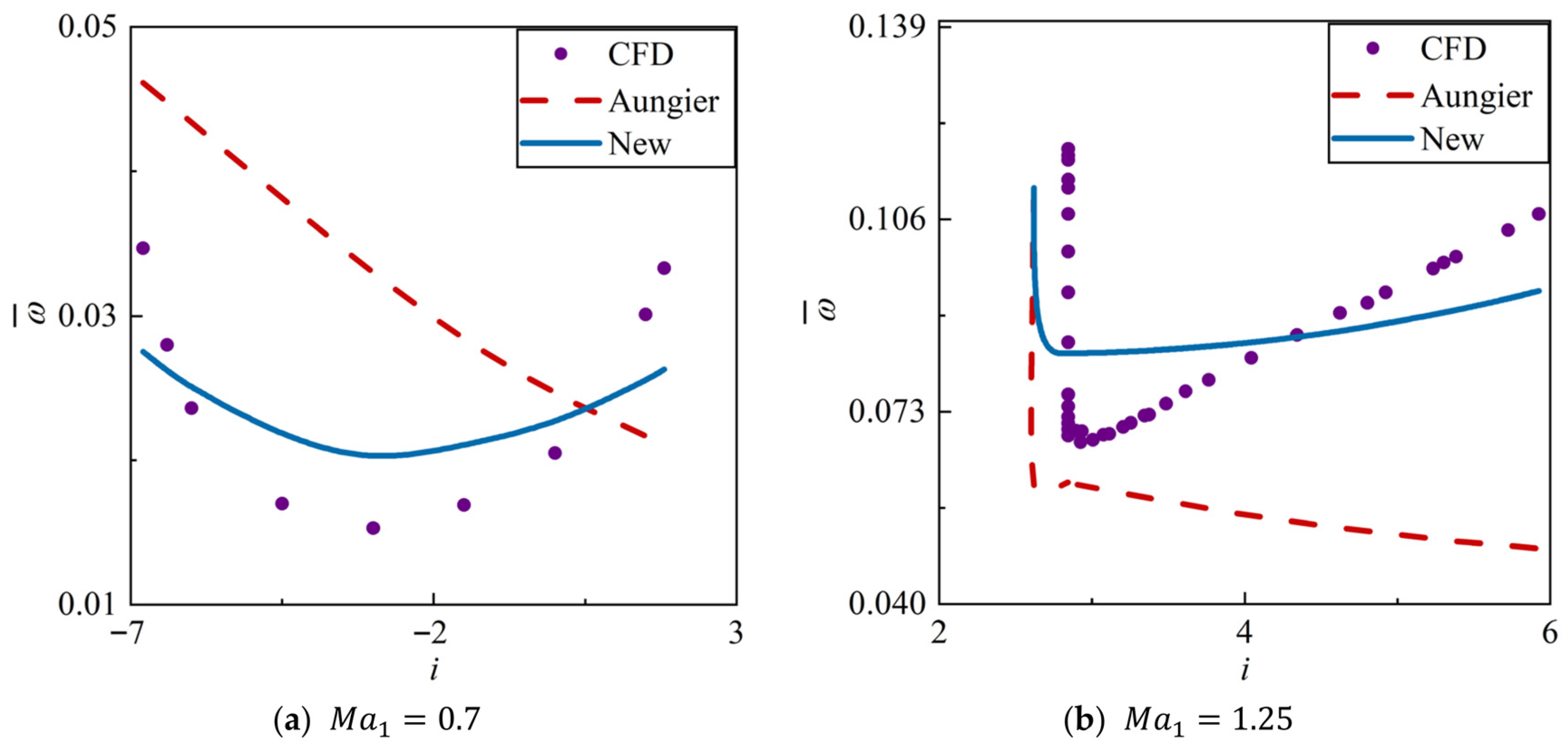
To further ensure the reliability of the numerical method for the database in this study, Computational Fluid Dynamics (CFD) results were validated against experimental data of typical cascades in this database. Figure 2 compares the i -total loss coefficient ( ω ¯ ) characteristic lines from CFD and experiments. For subsonic conditions ( M a 1 = 0.4 / 0.7 ), CFD accurately predicts the trend of ω ¯ variation with i , with all prediction errors within ±0.01. For the supersonic condition ( M a 1 = 1.25 ), characterized by a narrow stable operating range and complex flow field, experimental data were only available near the minimum loss condition due to measurement limitations. Nonetheless, the numerical method maintained acceptable prediction accuracy for the loss at this point with an error of 0.01. In conclusion, the numerical simulation method employed in this study demonstrates sufficient accuracy across various geometric and aerodynamic conditions, providing a solid data foundation for subsequent loss model system research.

3. Development of the Loss Model System for 2D CDA Cascades

This section details the development of the loss model system for 2D CDA cascades based on the database training set. It begins by overviewing the model system structure and summarizing the development approach for all sub-models, followed by detailed descriptions of the development process and results for each sub-model.

3.1. Model System Structure

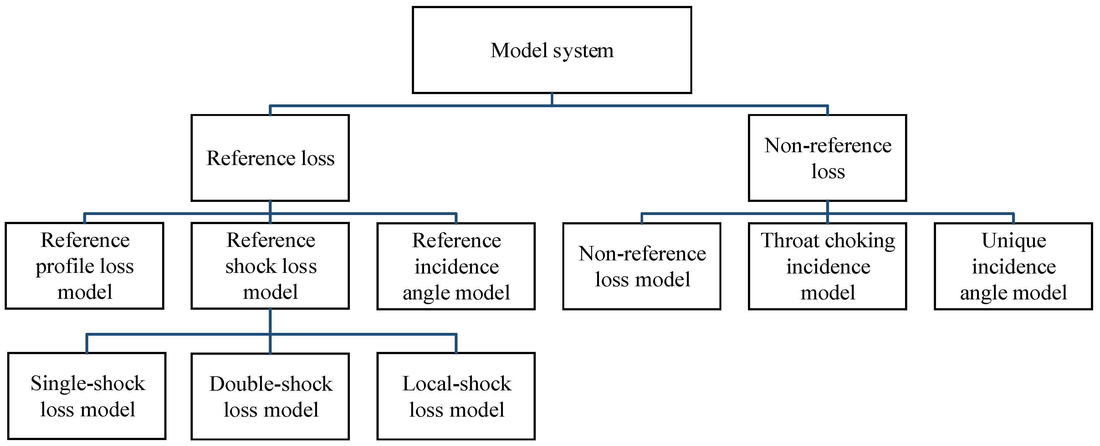
The overall structure of the proposed model system is shown in Figure 3. Since the system covers subsonic, transonic, and supersonic profiles, the 2D cascade loss consists of two parts: profile loss and shock loss. The profile loss mainly originates from blade surface boundary layer friction effects and wake mixing, while the shock loss is mainly caused by shock structures.
The system predicts the loss at reference points and non-reference points separately. The reference point is chosen as the minimum loss point, denoted by the superscript *. The cascade loss at reference points is predicted using the models for reference incidence angle ( i * ), reference profile loss ( ω ¯ p r o * ), and reference shock loss ( ω ¯ s h * ). The losses at other operating points are then modeled based on the reference data using the non-reference loss model. The reference shock loss model further includes sub-models for single-wave shock loss ( ω ¯ s h , s i n g l e * ), double-wave shock loss ( ω ¯ s h , d o u b l e * ), and local shock loss ( ω ¯ s h , l o c a l * ), targeting different shock wave structures. Additionally, because for high-speed profiles, the incidence angle cannot be less than the throat choking incidence angle ( i t h r o a t ) and the unique incidence angle ( i u n i q u e ), models for i t h r o a t and i u n i q u e are introduced to restrict the minimum incidence angle ( i m i n ), ensuring consistency with physical principles.
For each sub-model, a combined strategy of theoretical analysis and data-driven methods is employed: (1) Traditional models with solid physical foundations are selected as baselines based on theoretical analysis; (2) The GBM method is employed to guide baseline model optimization, by identifying the primary mechanisms responsible for the model prediction errors.

3.2. Reference Profile Loss Model

3.2.1. Baseline Model Formulation of Reference Profile Loss Model

The reference profile loss model in this paper is centered on the theoretical formula from the physically well-founded Lieblein model [6]:
ω ¯ p r o = 2 σ c o s β 2 c o s β 1 c o s β 2 2 · f w a k e
f w a k e * = θ w a k e * c 1 θ w a k e * c σ H w a k e * c o s β 2 * 3 ( 2 H w a k e * 3 H w a k e * 1 )
This formulation is derived by analyzing and modeling the blade wake velocity distribution at the reference point. However, the wake term f w a k e contains the unknown wake momentum thickness ( θ w a k e ) and shape factor ( H w a k e ), making the modeling of f w a k e the core challenge in predicting ω ¯ p r o .
Previous studies commonly correlate f w a k e with the diffusion factor ( D ) or equivalent diffusion factor ( D e q ) using polynomial relationships. Both D and D e q characterize blade load. The polynomial order can be as high as eight. D is generally calculated using Lieblein’s method, while Wright [11], Koch [7], and Lieblein [6] each proposed their own D e q calculation methods. To identify the most suitable f w a k e modeling approach for CDA profiles, a comprehensive evaluation of 1st- to 8th-order polynomial correlations was conducted based on the training set, using different load parameters ( D , D e q W r i g h t , D e q L i e b l e i n , and D e q K o c h ) as function arguments. The results (Table 2) indicate that the optimal choice is a 1st-order polynomial with D e q K o c h as the function argument:
f w a k e = 0.017 + 0.017 D e q K o c h
Its Root Mean Square Error (RMSE) is only 0.6% higher than that of the 8th-order polynomial, demonstrating that the lowest model complexity is sufficient to achieve accuracy comparable to high-order polynomials.
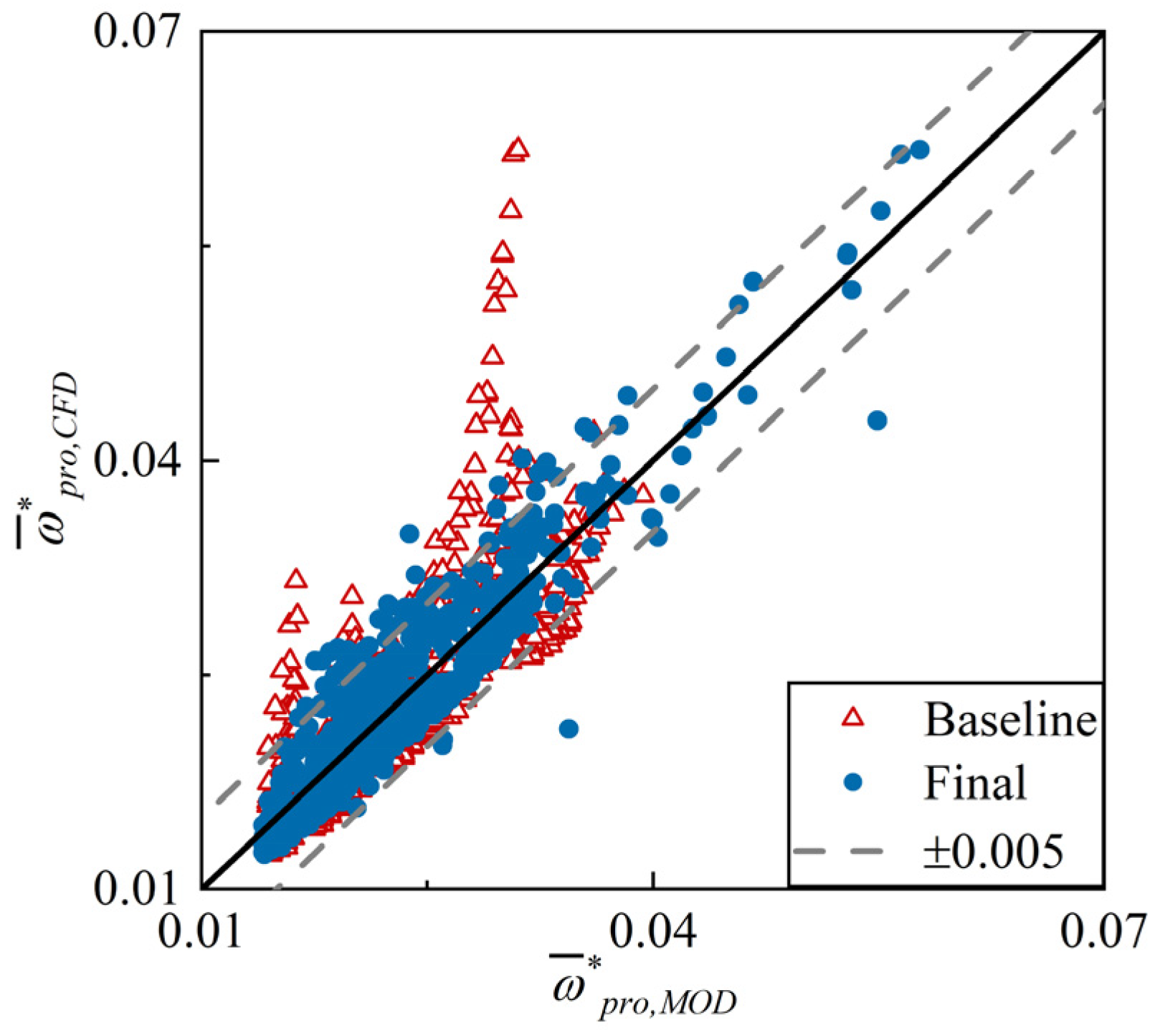
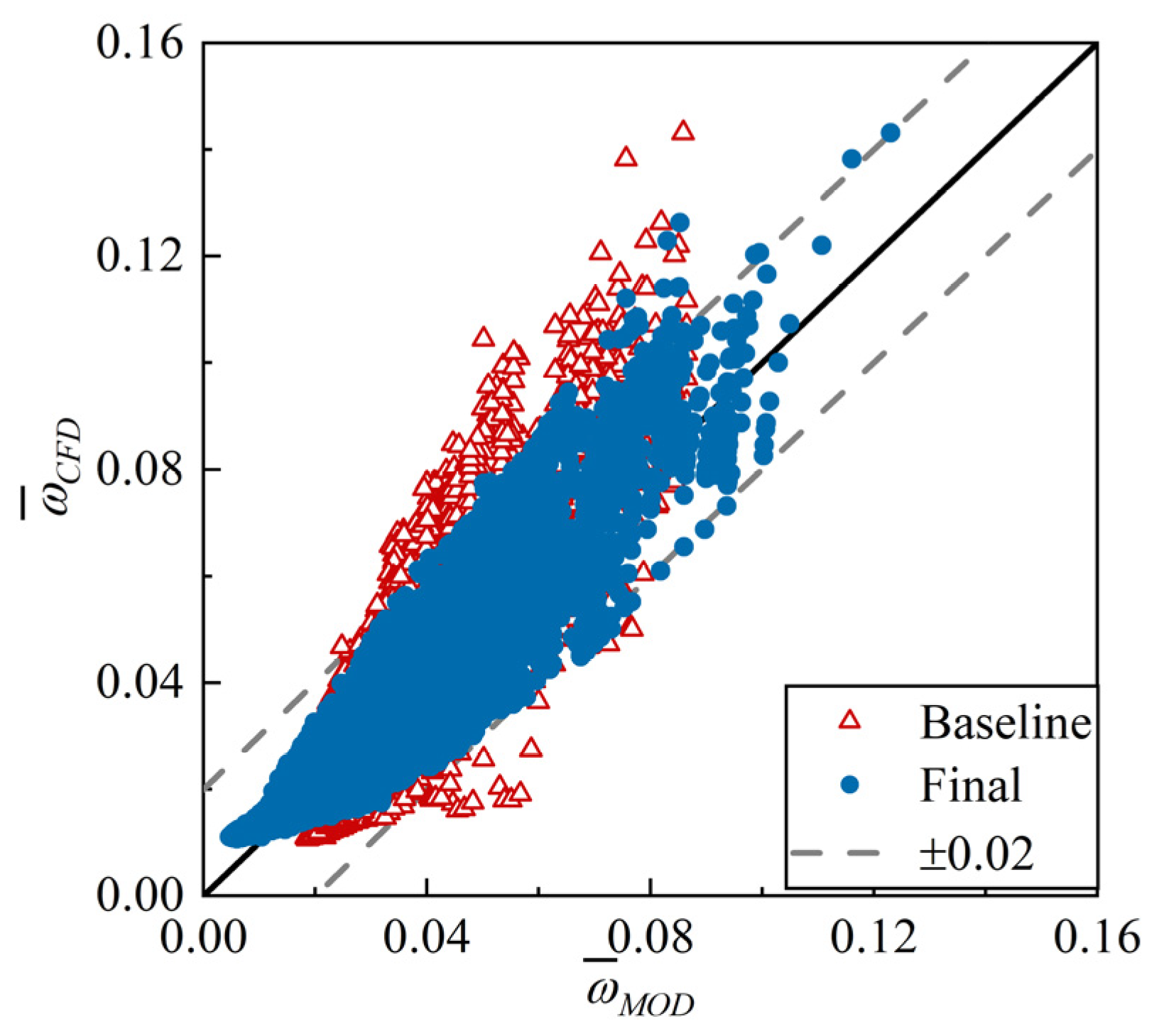
Equations (1) and (3) form the baseline ω ¯ p r o model. Figure 4 compares this baseline model (triangular markers) against CFD results. Table 3 quantitatively analyzes the model’s prediction accuracy using RMSE and the 95% Confidence Interval (95% CI) of the errors. The simple linear correlation is adequate for the majority of 2D cascades in the training set. For 95% of the samples, the absolute prediction error is less than 0.008 and the Pearson correlation coefficient between f w a k e and D e q K o c h is 0.82. These results prove a strong linear correlation between f w a k e and D e q K o c h for most CDA profiles, sufficient to support high-precision prediction of ω ¯ p r o .

3.2.2. Error Attribution Analysis for Baseline Model of Reference Profile Loss Model

However, 25 sample points still exhibit absolute errors ϵ r e s > 0.01 , with a relatively concentrated distribution (Figure 4), suggesting that certain important physical mechanisms are still not captured by the baseline model. Based on the database parameter space (Table 1), the potential influencing factors are listed as:
ϵ r e s = f ( M a 1 , β M 1 , β M 2 , σ , t m a x c , x t m a x c , w m a x c , x w m a x c , γ , r l e )
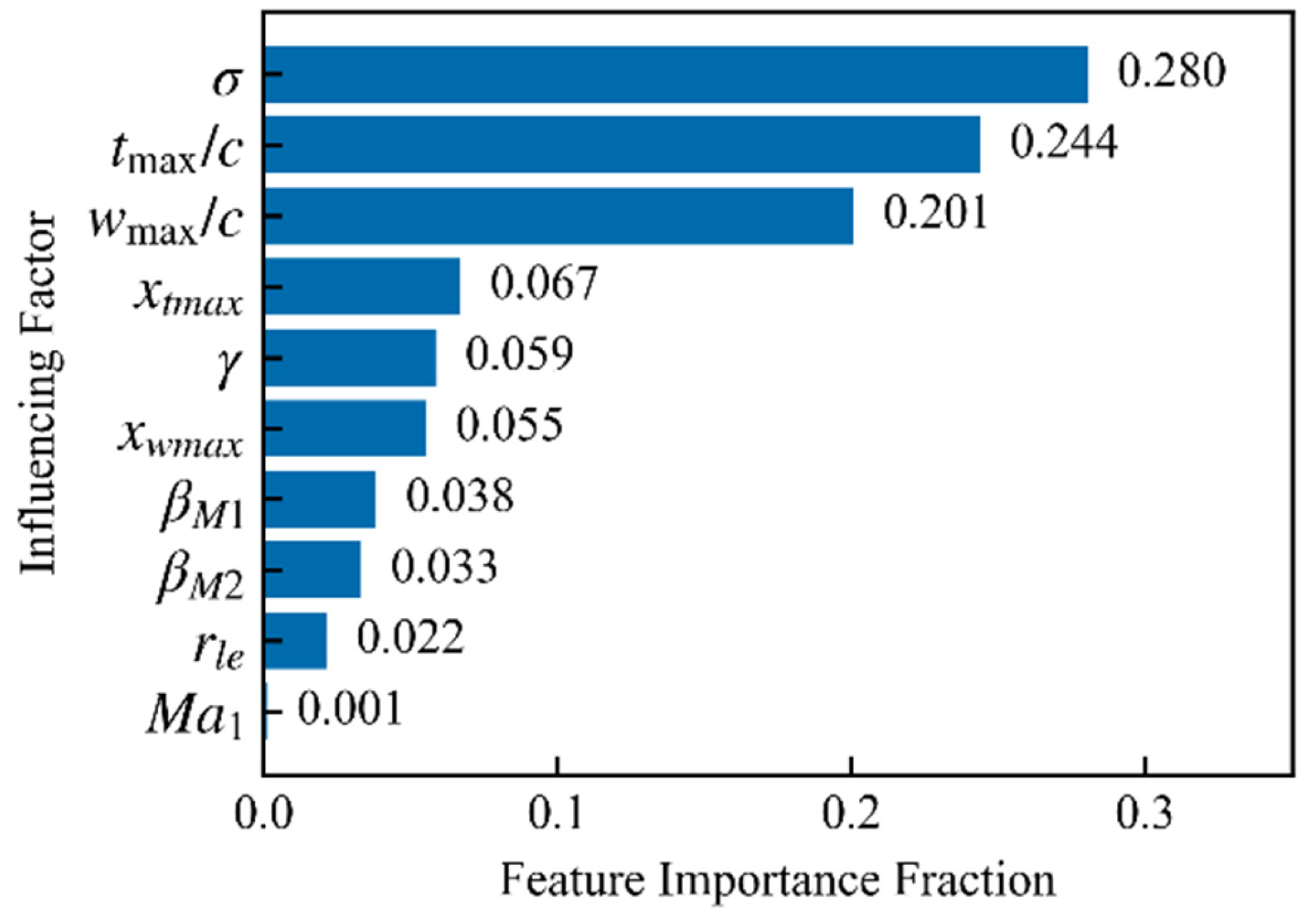
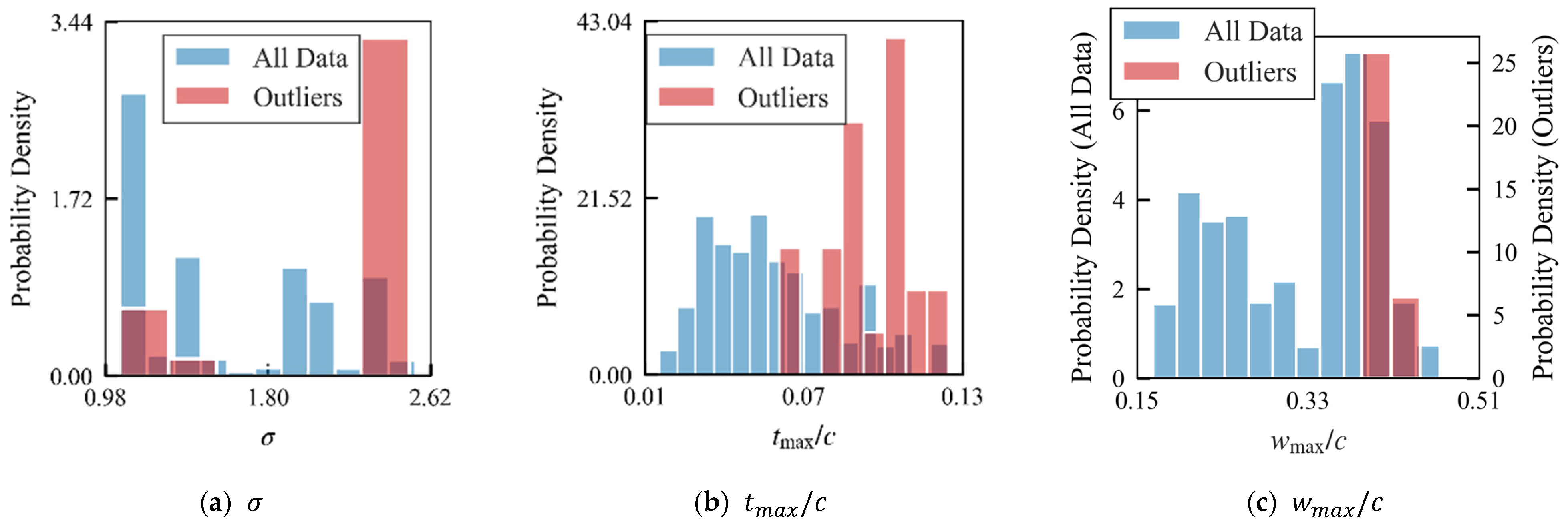
Quantitative attribution analysis on the errors of these outliers ( ϵ r e s > 0.01 ) was performed using the GBM method. The analysis revealed (Figure 5) that the effects of t m a x c , σ , and w m a x c are significantly higher than that of other parameters, collectively explaining over 78% of the prediction errors. Furthermore, it is observed that the values of t m a x c , σ , and w m a x c for these outliers are mostly concentrated at the edges of the parameter space (Figure 6). Specifically, t m a x c and w m a x c tend to approach their maximum values, while σ tends to approach either its maximum or minimum values. This suggests that relying solely on the blade load to model f w a k e is insufficient under some edge design conditions.
Excessively large t m a x c and w m a x c values increase geometric blockage, intensify flow turning, and consequently lead to increased local loading on the latter rear of the blade. This causes a stronger adverse pressure gradient, leading to rapid boundary-layer growth or even separation and thus significantly increases the blade wake loss. Excessively small σ weakens the flow diversion capability due to the wide blade passage, possibly inducing blade surface boundary layer separation and significantly increasing the blade wake loss. Excessively large σ increases the blade surface friction area, significantly increasing the blade surface boundary layer friction loss. However, Equation (3), modeled based only on the overall cascade load, fails to account for the changes in the axial distribution of the blade load, nor does it model blade surface boundary layer separation and friction effects. These limitations are the main reasons why the baseline model underestimates the ω ¯ p r o of some cascades.

3.2.3. Optimization and Validation of Reference Profile Loss Model

The formulation for f w a k e was adapted by incorporating the three critical influencing factors:
f w a k e = ( 0.01 + 0.01 + 5.36 × 10 4 t m a x c 3.02 σ 2.39 w m a x c 12.36 · D e q K o c h )
Combining Equation (5) with the theoretical part (Equation (1)) yields the final ω ¯ p r o model. The final model significantly enhances the applicability to edge designs (circular markers, Figure 4), with the number of outliers reduced by 88%. Around 95% of the absolute errors are less than 0.005, which means the model achieved a high prediction accuracy (Table 3). These results demonstrate that, by centering on a theoretical formula and identifying critical influencing factors, a concise yet physically meaningful model has been successfully constructed, accurately predicting ω ¯ p r o for 2D CDA cascades across a wide design space.

3.3. Reference Shock Loss Model

3.3.1. Baseline Model Formulation of Reference Shock Loss Model

The structure of the reference shock loss model in this paper is as follows:
ω ¯ s h = ω ¯ s h , l o c a l                                                                                                                   M a 1 < 1 k t r a n · ω ¯ s h , s i n g l e + ( 1 k t r a n ) · ω ¯ s h , d o u b l e           M a 1 > 1
For subsonic conditions, the local shock loss model is applied. For supersonic conditions, k t r a n is introduced to weight the single and double wave losses, modeling the complex shock wave structures within the cascade passage.
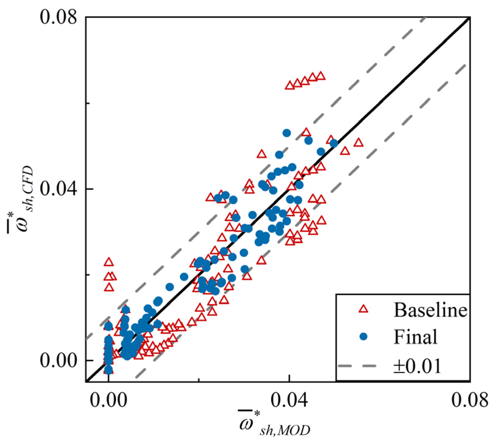
Modeling schemes with solid physical foundations were firstly selected from the literature for ω ¯ s h , l o c a l * , ω ¯ s h , s i n g l e * , ω ¯ s h , d o u b l e * , and k t r a n (Table 4). Different combinations of these schemes were then evaluated based on the database test set (Table 5). Results indicated that the combination of the Creveling ω ¯ s h , l o c a l * model [21], Aungier ω ¯ s h , s i n g l e * model [8], Koch ω ¯ s h , d o u b l e * model [7], and Hu k t r a n model [22] performed best (lowest RMSE) and was thus selected as the baseline ω ¯ s h * model. However, comparison with CFD results (Figure 7 and Table 6) showed that this baseline model still exhibited large errors for several sample points, suggesting the potential for further improvement in its prediction accuracy.

3.3.2. Optimization and Validation of Reference Shock Loss Model

Quantitative attribution analysis on the errors of the baseline ω ¯ s h * model was performed using the GBM method, showing that M a 1 is the most important influencing factor. During the model optimization process, it was found that the theoretical core of the predominantly theoretically-derived Creveling ω ¯ s h , l o c a l * model [21], Aungier ω ¯ s h , s i n g l e * model [8], and Koch ω ¯ s h , d o u b l e * model [7] remained applicable to CDA profiles. Significant performance improvement could be achieved merely by modifying the empirical estimation of the Mach number at the shock wave front ( M a s ) in these three models.
The modified wavefront Mach number of the Creveling ω ¯ s h , l o c a l * model [21] ( M a s , l o c a l ) decreases as M a 1 decreases:
M a s , l o c a l = m a x ( 3.5 M a 1 1 + M a b , l o c a l , M a 1 = 1 , 0 )
where M a b , l o c a l , M a 1 = 1 is the Mach number after the inlet flow (assumed to be sonic) expands isentropically to the wavefront location along the suction surface.
The wavefront Mach number of the Aungier ω ¯ s h , s i n g l e * model [8] ( M a s , l o c a l ) was slightly reduced:
M a s , s i n g l e = 0.95 M a b · M a 1
where M a b is the Mach number after the inlet flow expands isentropically to the wavefront location along the suction surface.
The wavefront Mach number in the Koch ω ¯ s h , d o u b l e * model [7] ( M a s , d o u b l e ) was slightly increased:
M a s , d o u b l e = 0.21 M a 1 + 1.21 M a m a x
where M a m a x is the peak Mach number on the suction surface.
However, the Hu k t r a n model [22], which simply distinguishes between single and double shocks with a Mach number boundary at M a 1 = 1.2 , causes an abrupt change in ω ¯ s h near this Mach number. This discontinuity is inconsistent with the smooth physical transition between different shock structures in the real flow. Consequently, a continuous function of M a 1 was introduced for modeling k t r a n :
k t r a n = 8.63 M a 1 2 20.86 M a 1 + 12.80
to achieve a smooth transition between different shock structures.
Integrating these four modified sub-models yields the final ω ¯ s h model. The final model no longer has excessively large prediction errors ( ϵ r e s m a x = 0.014 ), and the 95% confidence interval for error is [−0.0094, 0.0095] (Figure 7 and Table 6). These results indicate that for the shock models grounded on solid physical foundations, simply correcting the wavefront Mach number estimation successfully extends their applicability to CDA profiles. For empirical models, however, optimizing their algorithm is necessary to enhance their consistency with physical principles.

3.4. Throat Choking and Unique Incidence Angle Models

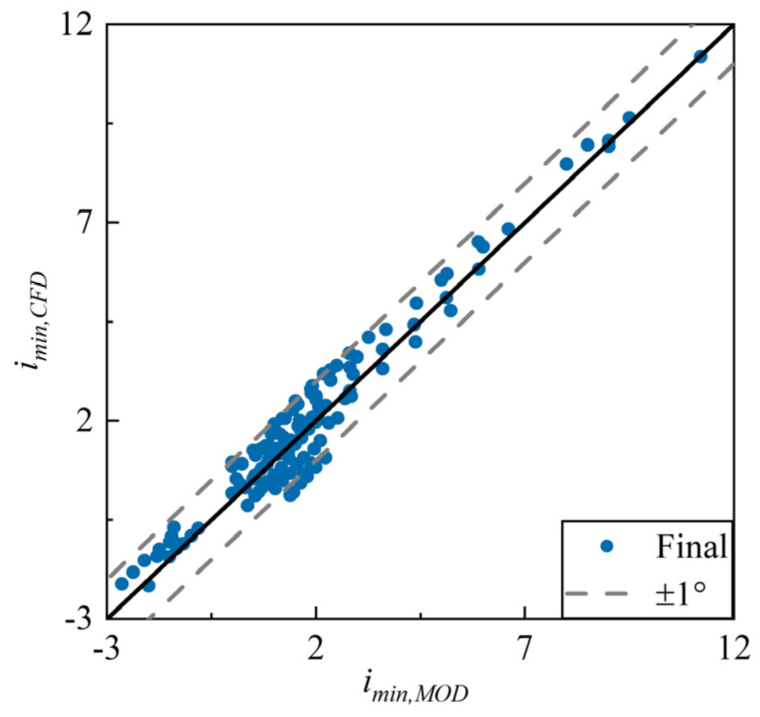
The study found that the Aungier throat choking incidence model [8] and the Levine unique incidence model [23], which are dominated by theoretical derivation with minimal reliance on empirical parameters, demonstrate good applicability to high-speed CDA profiles covering a wide design range. Accurate prediction of the minimum incidence angle ( i m i n ) was achieved without additional modifications:
i m i n = m i n ( i t h r o a t , i u n i q u e )
Validation results based on the training set (Figure 8 and Table 7) show a maximum prediction error of 1.28°, and approximately 95% of the prediction errors fall within the interval [−0.97°, 1.21°].

3.5. Reference Incidence Angle Model

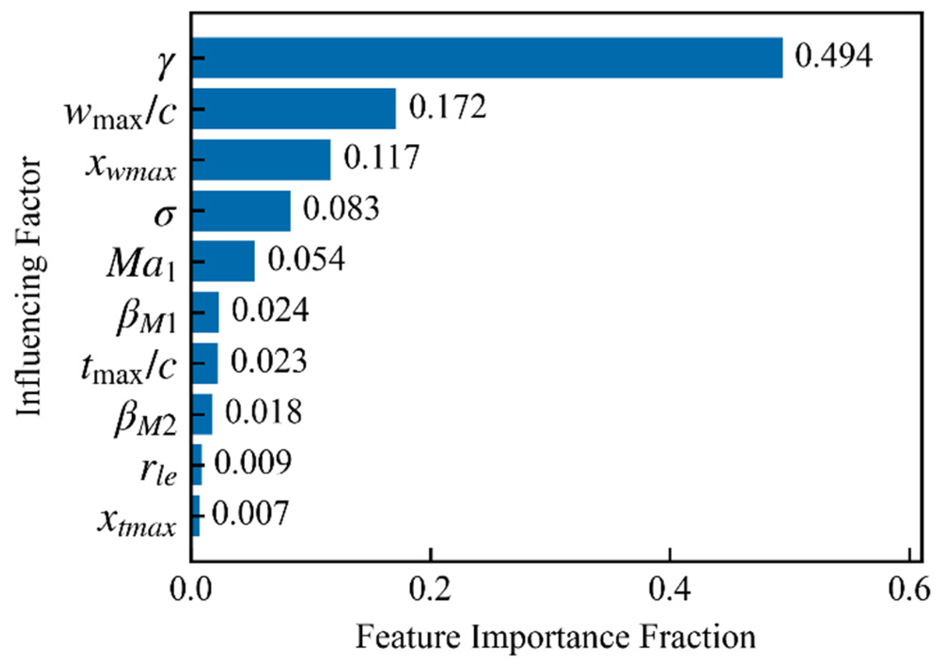
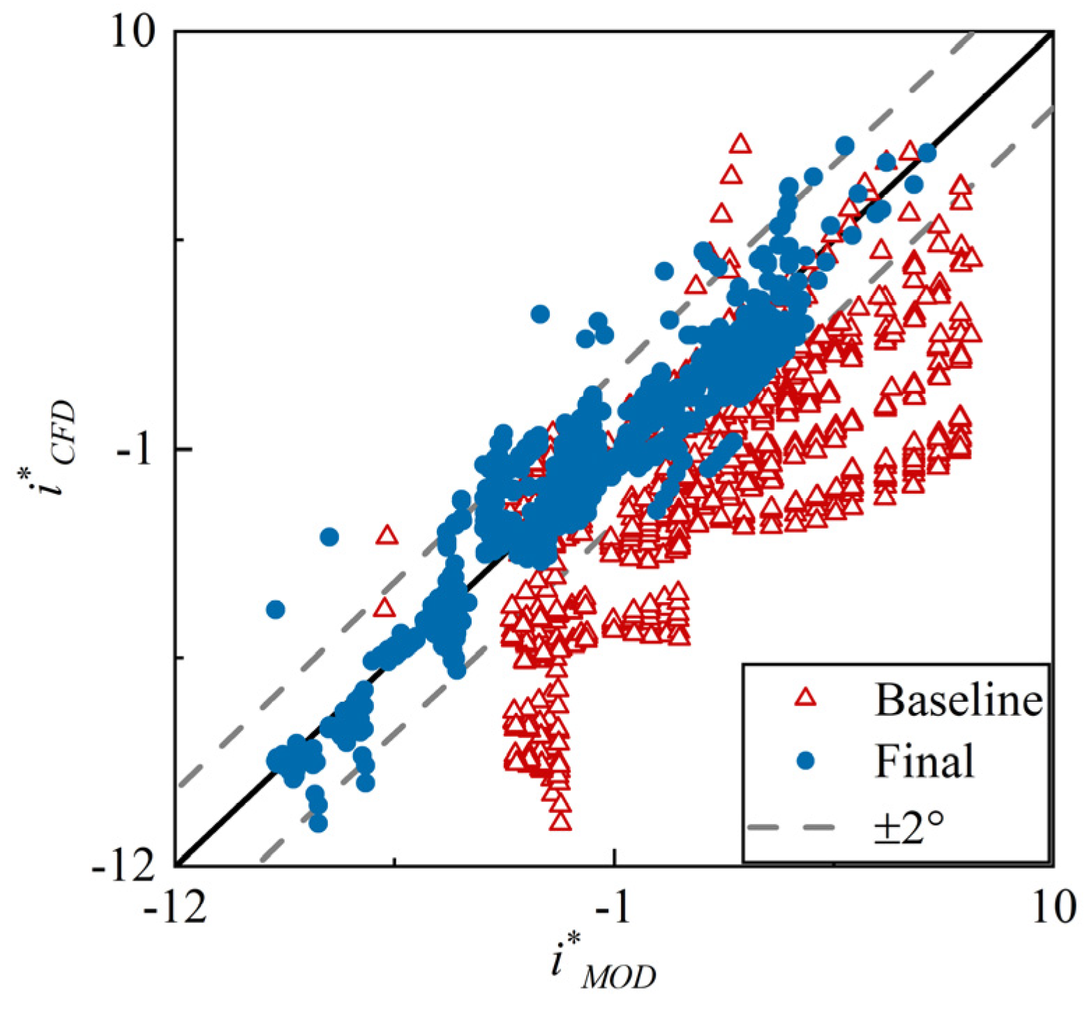
This study uses the widely adopted Lieblein i * model [24] as the baseline model and optimizes it for modern 2D CDA cascades. γ and x w m a x c are identified as the two most important parameters by the GBM method, collectively explaining 66% of the prediction error (Figure 9). γ is one of the core parameters determining the geometric shape of the cascade passage, directly affecting key flow field characteristics such as blade load distribution, shock position, and shock strength. x w m a x c significantly influences the blade loading type (front/mid/aft loading), thereby changing the blade load distribution and shock structure. These effects all influence the locations of reference points.
The baseline model was then corrected using these two parameters to obtain the final i * model:
i = 0.45 k t i 0 10 + n θ + 0.23 γ 0.10 0.36 x w m a x c 4.96 + 2.13
where k t , i 0 10 , and n are parameters from the Lieblein model [24]. As shown in Figure 10 and Table 8, the final model improves the prediction accuracy by over 60% compared to the baseline model, with 95% of the absolute errors being less than 2 degrees. The results indicate that by identifying key influencing factors and introducing a concise correction term using only two geometric parameters, the new model significantly enhances its applicability to 2D CDA cascades. Subsequent validation (Section 4) will confirm that the accuracy of this model meets the requirements of loss prediction in modern 2D CDA cascades.

3.6. Non-Reference Loss Model

In traditional model systems, the non-reference point losses generally follow a quadratic function with respect to incidence angle, which is adopted as the baseline model in this paper. The critical factors influencing the error were then identified using the GBM method, leading to the final ω ¯ model:
ω ¯ = ω ¯ p r o + ω ¯ s h + 6.14 M a 1 + 5.96 i i 2 0.03 + 0.13 M a 1 σ + 4.12 × 10 4 β M 1
For independently evaluating the performance of this non-reference loss model, the reference point variables (including ω ¯ p r o * , ω ¯ s h * , and i * ) used for validation in this section are taken directly from CFD results rather than from the other sub-model predictions. The synergy among sub-models will be verified in Section 4. Figure 11 and Table 9 show that the final model improves accuracy by approximately 30% compared to the baseline model, with about 95% of the errors falling within ±0.015.

4. Validation of the Loss Model System for 2D CDA Cascades

This section presents a systematic validation of the entire loss model system for 2D CDA cascades developed in Section 3, using bothtraining and test set of the database. The performance of the new model system is also compared with that of the classical Aungier model system [8]. In the Aungier system [8], the reference profile loss model is based on the Lieblein theoretical formula [6] (the same as in the new system), but its wake term was developed using low-speed experimental data of traditional profiles such as NACA65 and C4; the reference shock loss model includes only a single-wave model [9] and does not consider variations in shock structures; the reference incidence angle model employs the original Lieblein correlation based on low-speed experimental data of traditional profiles [24]; the unique-incidence and throat-choking models [8,23] are identical to those in the new system; the non-reference loss model consists of three empirical sub-models—the stall incidence angle model [8], the choke incidence angle model [8], and the loss-incidence-variation model [8]—resulting in a much more complex formulation compared with the single correlation used in the new model system.

4.1. Validation on the Training Set

Section 3 only independently evaluated each sub-model using the database training set. Therefore, this section validates the integrated model system to assess the synergy between the sub-models.
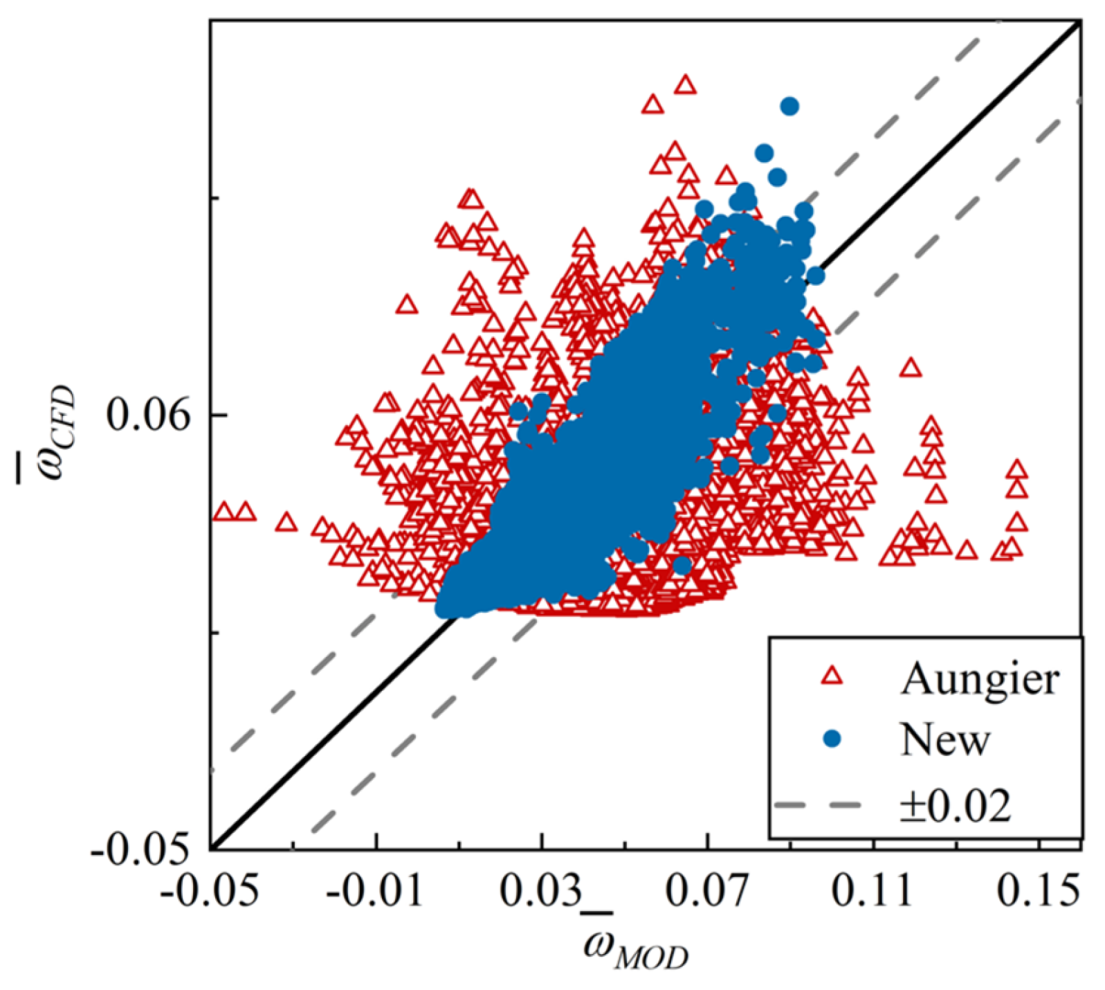
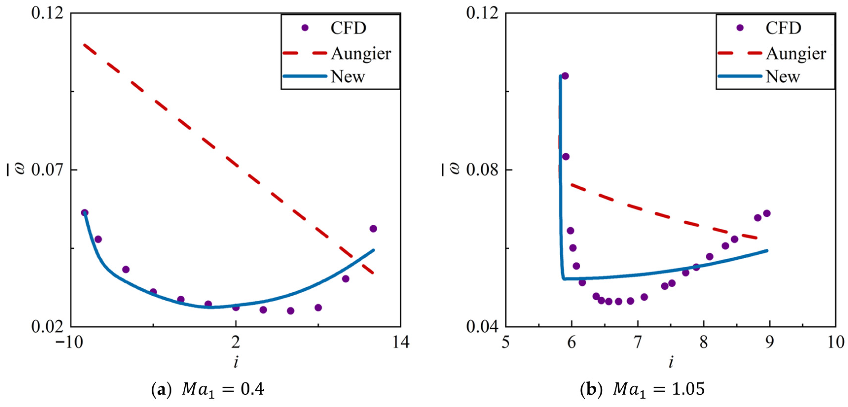
Figure 12 compares the predictions of the Aungier [8] and the new model systems against CFD results. Table 10 provides quantitative evaluation for the prediction accuracy of both systems, employing Mean Absolute Error (MAE), Root Mean Square Error (RMSE), Coefficient of Determination (R2), and the 95% Confidence Interval (CI) of the error. The results indicate that the new model system is more suitable for modern CDA profiles. The RMSE is improved by 75%. Approximately 95% of the absolute errors are less than 0.016. Furthermore, as shown in Figure 13, for subsonic, transonic, and supersonic CDA cascades, the predicted loss trends with incidence angle agree well with the CFD results, including the boundary of minimal incidence angles for high-speed cascades, while the Aungier system does not [8].
The above results demonstrate that all sub-models work well together, exhibiting better applicability and accuracy than the Aungier model system [8] for 2D CDA cascades across a wide design space.

4.2. Validation on the Test Set

This section further validates the extrapolation capability of the new loss model system using the database test set.
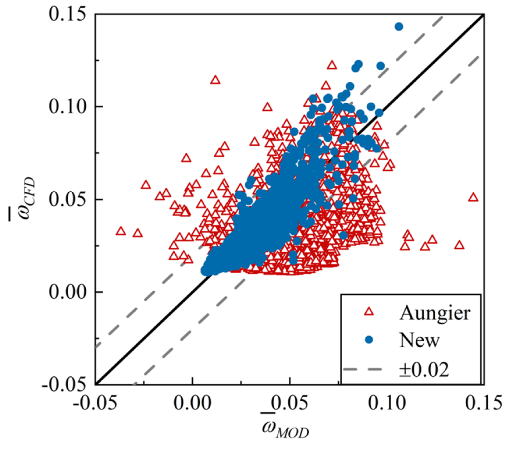
Figure 14 and Table 11 compare the Aungier [8] and the new model systems. The new system achieves a prediction accuracy on the test set comparable to that on the training set, and is much more accurate than the Aungier model system. The R2 value is 0.76, and 95% of the prediction errors fall within the interval [−0.018, 0.018]. Furthermore, Figure 15 presents the incidence-loss characteristic lines for typical subsonic, transonic, and supersonic cascades in the test set. The new model system successfully predicts the loss trend with incidence angle, including the minimum incidence boundary for high-speed profiles.
These results confirm that the new model system exhibits good extrapolation capability and accuracy when applied to unseen CDA profiles.

4.3. Validation Against Experimental Data

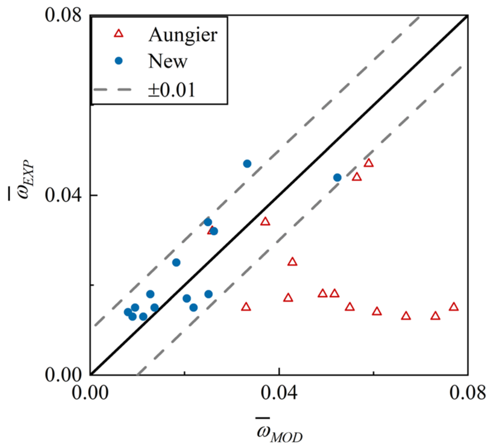
To further evaluate the accuracy and reliability of the new loss model system in real cascade flow environments, additional validation was conducted using the available experimental data of 2D CDA cascades, which have been presented in Figure 2. Figure 16 compares the predicted loss of both Aungier [8] and new model systems against experimental measurements, and Table 12 provides quantitative comparison of their prediction accuracy. The new model system shows significantly improved accuracy over the Aungier system for the three experimental cascades, with 93% of absolute errors below 0.01.
Figure 17 illustrates the capability of both model systems in predicting the variation of loss with incidence angle. For subsonic cascades ( M a 1 < 1 ), the new model system accurately captures the trend, while the Aungier system [8] fails. For the supersonic cascade ( M a 1 = 1.25 ), due to the limitations in experimental measurement techniques, the available data only cover operating conditions near the minimum-loss point (as discussed in Section 2.2). Although this data cannot fully represent the entire variation trend of loss across the incidence range, it remains valuable for validating model accuracy near the design condition of the supersonic cascade. At this measured point, the new model system provides a more accurate loss prediction.
In summary, the new model system exhibits significantly improved prediction accuracy compared to the Aungier system [8], further confirming its applicability for 2D CDA cascades.

5. Conclusions

Based on traditional loss models, this paper develops a more comprehensive loss model system for two-dimensional (2D) cascades with modern Controlled Diffusion Profile (CDA) by combining physical analysis with data-driven methods. The new model system demonstrates good prediction accuracy across wide design spaces and the entire operating range, providing an efficient and reliable loss-prediction tool for the design and analysis of modern compressor profiles. The main conclusions are as follows:
  • A wide-range numerical simulation database for 2D CDA cascades was constructed. The database contains 920 cascade configurations and 9426 operating points, covering flow states from subsonic to supersonic (inlet Mach number 0.4–1.4), the full operating range from stall to choke (incidence angle −23° to 19°), and various profile designs, from low to high loading, front-loaded to aft-loaded, and so on. This provides a solid data foundation for the development and validation of the new model system.
  • New models were obtained by applying data-driven techniques to optimize traditional models with solid physical foundations. The study found that the theoretical core of the traditional models remains applicable to CDA profiles, but their empirical correlations are generally inadequate. The Gradient Boosting Machine method was introduced to perform quantitative attribution analysis on the model errors, identifying critical influencing factors for targeted optimization. Employing this method, significant accuracy improvement was achieved merely through simple modifications to the formulas.
  • Important mechanisms influencing the modeling of reference profile loss for 2D CDA cascades were revealed. For the majority of CDA cascades in the database, a distinct linear correlation exists between the equivalent diffusion factor and the critical wake term in the reference profile loss model. Additionally, variations in the axial load distribution, as well as blade surface boundary layer separation and friction effects, have a non-negligible influence on the loss prediction for part of the profiles located at the edges of the parameter space.
  • An all-operation loss model system for 2D CDA cascades was developed. The system is composed of a series of explicit expressions with clear physical significance. Across all the data, about 95% of the absolute prediction errors are less than 0.018. The new model reduces the RMSE by over 77% compared to the classical Aungier model system [8], demonstrating its superior accuracy.

Author Contributions

Conceptualization, X.Y. (Xianjun Yu) and B.L.; methodology, X.Y. (Xiang Yan); investigation, X.Y. (Xiang Yan); writing—original draft preparation, X.Y. (Xiang Yan); writing—review and editing, G.A. and R.W.; supervision, B.L. All authors have read and agreed to the published version of the manuscript.

Funding

This research was supported by the China Space Foundation (No. KDJJ20240202004).

Institutional Review Board Statement

Not applicable.

Informed Consent Statement

Not applicable.

Data Availability Statement

The data presented in this study is available on request from the corresponding author.

Conflicts of Interest

The authors declare no conflicts of interest.

Nomenclature

Symbols
c Chord length
D Diffusion factor
D e q Equivalent diffusion factor
f w a k e Blade wake term in the reference profile loss model
H w a k e Blade wake shape factor
i Incidence angle
i 0 10 Reference incidence angle of NACA65 profile with 0° camber angle and 10% maximum relative thickness
i m i n Minimum incidence angle
i t h r o a t Throat choking incidence angle
i u n i q u e Unique incidence angle
k t Correction factor for maximum relative thickness
k t r a n Weighting factor for reference shock loss
M a Mach number
M a b Mach number after isentropic expansion to the shock wave front along the suction surface
M a m a x Peak Mach number on the suction surface
M a s Mach number at the shock wave front
n Correction factor for camber angle
r l e Leading edge radius
t m a x Maximum thickness
w m a x Maximum deflection
x t m a x Chordwise position of maximum thickness
x w m a x Chordwise position of maximum deflection
β Flow angle
β M Metal angle
γ Stagger angle
θ M Camber angle
θ w a k e Blade wake momentum thickness
σ Solidity
ω ¯ Total pressure loss
ω ¯ p r o Profile loss
ω ¯ s h Shock loss
ω ¯ s h , d o u b l e Double-wave shock loss
ω ¯ s h , l o c a l Local shock loss
ω ¯ s h , s i n g l e Single-wave shock loss
ϵ r e s Model prediction error
Subscripts
1Inlet
2Outlet
d e Parameter at the design point
CFDNumerical result
EXPExperimental result
MODModel prediction result
Superscripts
*Parameter at the reference point

References

  1. Senior, A.C.; Miller, R. Improving Compressor Preliminary Design with Physically Decomposed Loss Models. J. Turbomach. 2026, 148, 021007. [Google Scholar] [CrossRef]
  2. Guo, Z. The Study of Transition on Controlled Diffusion Airfoils Using Large Simulations; Shanghai Jiao Tong University: Shanghai, China, 2020. [Google Scholar]
  3. Hobbs, D.; Weingold, H. Development of controlled diffusion airfoils for multistage compressor application. J. Eng. Gas Turbines Power 1984, 106, 271–278. [Google Scholar] [CrossRef]
  4. Rechter, H.; Steinert, W.; Lehmann, K. Comparison of controlled diffusion airfoils with conventional NACA 65 airfoils developed for stator blade application in a multistage axial compressor. J. Eng. Gas Turbines Power 1985, 107, 494–498. [Google Scholar] [CrossRef]
  5. Behlke, R. The development of a second generation of controlled diffusion airfoils for multistage compressors. J. Turbomach. 1986, 108, 32–40. [Google Scholar] [CrossRef]
  6. Lieblein, S. Loss and stall analysis of compressor cascades. J. Basic Eng. 1959, 81, 387–397. [Google Scholar] [CrossRef]
  7. Koch, C.C.; Smith, L.H. Loss sources and magnitudes in axial-flow compressors. J. Eng. Gas Turbine. Power 1976, 98, 411–424. [Google Scholar] [CrossRef]
  8. Aungier, R.H. Axial-Flow Compressors: A Strategy for Aerodynamic Design and Analysis; American Society of Mechanical Engineers: New York, NY, USA, 2003. [Google Scholar]
  9. Miller, G.R.; Lewis, G.W., Jr.; Hartmann, M.J. Shock losses in transonic compressor blade rows. J. Eng. Power. 1961, 83, 235–241. [Google Scholar] [CrossRef]
  10. Boyer, K.M.; O’Brien, W.F. An improved Streamline Curvature Approach for Off-Design Analysis of Transonic Axial Compression Systems. J. Turbomach. 2003, 125, 475–481. [Google Scholar] [CrossRef]
  11. Wright, P.I.; Miller, D.C. Improved compressor performance prediction model. In Proceedings of the European Conference on Turbomachinery, London, UK, 19–20 March 1991; pp. 69–82. [Google Scholar]
  12. Sun, X.; Yang, S.; Zhao, Q. Shock loss model and blade profile optimization design of a supersonic cascade. Proc. Inst. Mech. Eng. Part G J. Aerosp. Eng. 2015, 229, 1325–1329. [Google Scholar] [CrossRef]
  13. Banjac, M.; Savanovic, T.; Petkovic, D.; Petrovic, M.V. A comprehensive analytical shock loss model for axial compressor cascades. J. Turbomach. 2022, 144, 091003. [Google Scholar] [CrossRef]
  14. Hearsey, R.M. Program HT0300 NASA 1994 Version; The Boeing Company: Seattle, WA, USA, 1994. [Google Scholar]
  15. Tao, H.Q.; Xu, N.; Li, R.Z.; Jiang, B. Research on Loss and Deviation Angle Model based on Multivariate Nonlinear Regression. Therm. Energy Power Eng. 2022, 37, 38–46. [Google Scholar]
  16. Tao, C.; Du, X.; Ding, J.; Luo, Y.; Wang, Z. Maximum thickness location selection of high subsonic axial compressor airfoils and its effect on aerodynamic performance. Front. Energy Res. 2021, 9, 791542. [Google Scholar] [CrossRef]
  17. Fei, T. Investigation on through-flow analysis framework and empirical model improvement of high-load compressors. Ph.D. Thesis, Beijing Institute of Technology, Beijing, China, 2020. [Google Scholar]
  18. Yue, Z.; Zhou, C.; Jin, D.; Gui, X. A spanwise loss model for axial compressor stator based on machine learning. Chin. J. Aeronaut. 2022, 35, 74–84. [Google Scholar] [CrossRef]
  19. Shi, H. Study on Design Method of Super/Transonic Compressor Airfoil and Application; Beihang University: Beijing, China, 2019. [Google Scholar]
  20. Ning, F.F. Numerical Simulation of Internal Flows in Transonic Compressors with Actual Geometric Fidelity; Beihang University: Beijing, China, 2002. [Google Scholar]
  21. Creveling, H.F.; Carmody, R.H. Axial Flow Compressor Computer Program for Calculating off Design Performance (Program IV); NASA-CR-72427; NASA: Washington, DC, USA, 1968. [Google Scholar]
  22. Zhao, Y.; Hu, J. Analysis of the influence of inlet flow distortion on the off-design performance of fan/booster. J. Aerosp. Power 2007, 22, 1087–1092. [Google Scholar] [CrossRef]
  23. Levine, P. Two-dimensional inflow conditions for a supersonic compressor with curved blades. J. Appl. Mech. 1957, 24, 165–169. [Google Scholar] [CrossRef]
  24. Lieblein, S. Incidence and deviation-angle correlations for compressor cascades. J. Basic Eng. 1960, 82, 575–584. [Google Scholar] [CrossRef]
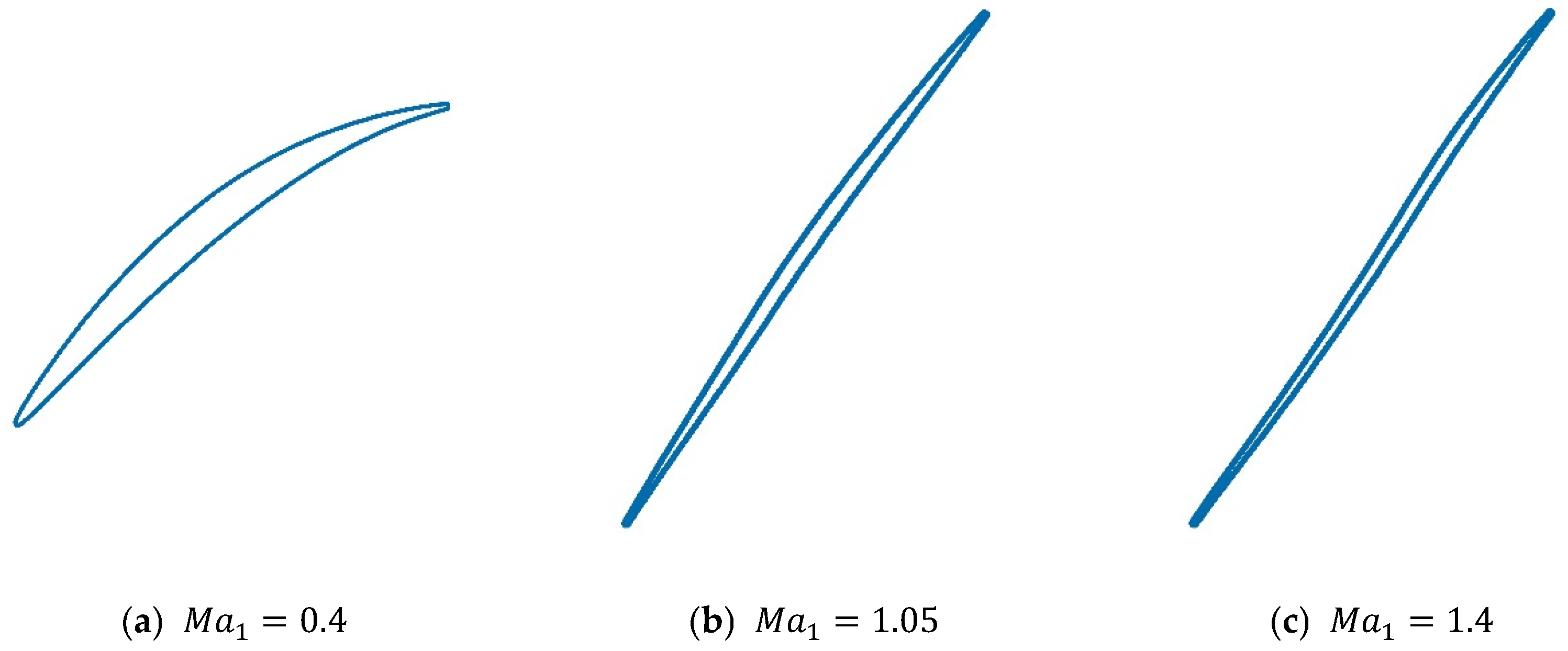
Figure 1. Typical subsonic, transonic, and supersonic CDA profiles.
Applsci 15 11759 g001
Figure 2. Validation of the numerical method against experimental data.
Applsci 15 11759 g002
Figure 3. Structure of the loss model system for 2D CDA Cascades.
Applsci 15 11759 g003
Figure 4. Comparison of baseline and final ω ¯ p r o models with CFD results.
Applsci 15 11759 g004
Figure 5. Quantitative attribution analysis of the baseline ω ¯ p r o model error.
Applsci 15 11759 g005
Figure 6. Location of critical factors for the outlier points within the database parameter range.
Applsci 15 11759 g006
Figure 7. Comparison of baseline and final ω ¯ s h * models with CFD results.
Applsci 15 11759 g007
Figure 8. Comparison of i t h r o a t and i u n i q u e models with CFD results.
Applsci 15 11759 g008
Figure 9. Quantitative attribution analysis of the baseline i model error.
Applsci 15 11759 g009
Figure 10. Comparison of baseline and final i models with CFD results.
Applsci 15 11759 g010
Figure 11. Comparison of baseline and final ω ¯ models with CFD results.
Applsci 15 11759 g011
Figure 12. Comparison of the Aungier and the new model systems for the training set [8].
Applsci 15 11759 g012
Figure 13. Comparison of loss variation with incidence angle for typical cascades in the training set [8].
Applsci 15 11759 g013
Figure 14. Comparison of the Aungier and the new model systems for the test set [8].
Applsci 15 11759 g014
Figure 15. Comparison of loss variation with incidence angle for typical cascades in the test set [8].
Applsci 15 11759 g015
Figure 16. Comparison of the Aungier and the new model systems on the experimental data [8].
Applsci 15 11759 g016
Figure 17. Comparison of loss variation with incidence angle for typical cascades for experimental cascades [8].
Applsci 15 11759 g017
Table 1. Parameter space of the numerical simulation database for 2D CDA cascades.
ParameterRange
i /(°)−23–19
M a 1 0.4–1.4
D d e 0.36–0.63
β M 1 /(°)32–75
β M 2 /(°)0–57
γ /(°)16–61
σ 1.05–2.55
t m a x / c 0.02–0.12
x t m a x / c 0.17–0.68
w m a x / c 0.18–0.50
x w m a x / c 0.35–0.78
r l e /(mm)0.24–1.63
Table 2. RMSE values for f w a k e modeling methods with different function arguments and polynomial orders.
Polynomial Order1278
D e q K o c h 2.43 × 10−32.43 × 10−32.42 × 10−32.42 × 10−3
D e q L i e b l e i n 2.73 × 10−32.73 × 10−32.66 × 10−32.61 × 10−3
D e q W r i g h t 2.45 × 10−32.45 × 10−32.42 × 10−32.42 × 10−3
D 2.79 × 10−32.79 × 10−32.70 × 10−32.70 × 10−3
Table 3. Quantitative analysis of prediction accuracy for the baseline and final ω ¯ p r o models.
Baseline   ω ¯ p r o * Model Final   ω ¯ p r o * Model
RMSE0.00430.0026
95% CI of errors[−0.0083, 0.0084][−0.0050, 0.0051]
Table 4. Candidate sub-models for ω ¯ s h * .
ω ¯ s h , l o c a l * ω ¯ s h , s i n g l e * ω ¯ s h , d o u b l e * k t r a n
Aungier [8]
Creveling [21]
Wright [11]
Miller [9]
Aungier [8]
Koch [7]Hu [22]
Table 5. Comparison of prediction accuracy for different ω ¯ s h * sub-model combinations.
Aungier [8]Miller [9]
Aungier [8]8.71 × 10−39.45 × 10−3
Creveling [21]8.71 × 10−39.44 × 10−3
Wright [11]8.81 × 10−39.67 × 10−3
Table 6. Quantitative analysis of prediction accuracy for the baseline and final ω ¯ s h * models.
Baseline   ω ¯ s h * Model Final   ω ¯ s h * Model
RMSE0.00890.0048
95% CI of errors[−0.017, 0.018][−0.0094, 0.0095]
Table 7. Quantitative analysis of prediction accuracy for i t h r o a t and i u n i q u e models.
i t h r o a t  and   i u n i q u e Models
RMSE0.57
95% CI of errors[−0.97°, 1.21°]
Table 8. Quantitative analysis of prediction accuracy for the baseline and final i models.
Baseline   i * Model Final   i * Model
RMSE3.851.01
95% CI of errors[−1.90°, 7.81°][−1.99°, 1.97°]
Table 9. Quantitative analysis of prediction accuracy for the baseline and final ω ¯ models.
Baseline   ω ¯ Model Final   ω ¯ Model
RMSE0.0110.0074
95% CI of errors[−0.021, 0.021][−0.015, 0.014]
Table 10. Quantitative analysis of prediction accuracy for the Aungier and the new model systems on the training set [8].
AungierNew
MAE0.0290.0064
RMSE0.0330.0083
R2−2.380.78
95% CI of errors[−0.027, 0.071][−0.016, 0.016]
Table 11. Quantitative analysis of prediction accuracy for the Aungier and the new model systems on the test set [8].
AungierNew
MAE0.0290.0066
RMSE0.0330.0088
R2−2.550.76
95% CI of errors[−0.023, 0.069][−0.018, 0.018]
Table 12. Quantitative analysis of prediction accuracy for the Aungier and the new model systems on the experimental data [8].
AungierNew
MAE0.0290.0066
RMSE0.0330.0088
R2−2.550.76
95% CI of errors[−0.023, 0.069][−0.018, 0.018]
Disclaimer/Publisher’s Note: The statements, opinions and data contained in all publications are solely those of the individual author(s) and contributor(s) and not of MDPI and/or the editor(s). MDPI and/or the editor(s) disclaim responsibility for any injury to people or property resulting from any ideas, methods, instructions or products referred to in the content.