Article

Constructing Emission-Intensive Driving Cycles for an Extended-Range Electric Vehicle via Dynamic Programming Guided by Real-World Trip Dynamics and Road Terrain

1
College of Mechanical and Vehicle Engineering, Chongqing University, Chongqing 400044, China
2
China Automotive Engineering Research Institute Co., Ltd., Chongqing 401122, China
3
Chongqing Changan Automobile Co., Ltd., Chongqing 400023, China
*
Author to whom correspondence should be addressed.
Appl. Sci. 2025, 15(21), 11762; https://doi.org/10.3390/app152111762
Submission received: 26 September 2025 / Revised: 24 October 2025 / Accepted: 31 October 2025 / Published: 4 November 2025

Abstract

Reproducing severe emission driving scenarios on a chassis dynamometer enables the systematic calibration of real driving emissions (RDE) under laboratory conditions. Accordingly, a dynamic programming (DP) method is proposed to construct emission-intensive driving cycles for an extended-range electric vehicle. The DP approach transforms the driving cycle construction problem into one of multi-stage decision optimization within a time control domain. Assembling a real driving emission model and a multi-stage decision optimization model, a DP algorithm was developed. Guided by real-world trip dynamics and road terrain, the DP algorithm optimizes instantaneous vehicle driving conditions at every time step, thereby reconstructing vehicle speed and road gradient profiles to maximize pollutant emissions within the time control domain. Analysis demonstrates that the DP algorithm favors constructing emission-intensive driving cycles using high-frequency, low-intensity acceleration and deceleration maneuvers, in addition to the high-aggression driving typically assumed to cause the severest emissions. Furthermore, the DP algorithm also effectively utilizes the impact of road terrain on emissions to construct these driving cycles. Verification confirms that the constructed emission-intensive driving cycles not only exhibit severe emission characteristics but also conform to the mandatory RDE test requirements in trip dynamics and road terrain conditions.

1. Introduction

Historically, vehicle emission control has been guided by a series of regulations established by governments and international organizations [1,2,3]. In compliance with these standards, a test vehicle is typically placed on a chassis dynamometer and subjected to emission testing according to a specified driving cycle. The driving cycle defines a speed profile, including idling, acceleration, constant speed, and deceleration, to approximate real-world driving conditions. The development of a representative driving cycle involves synthesizing real-world driving data into a standardized velocity-time profile. The process begins by extracting characteristic short-trips, often via clustering analysis of real-world driving data. These characteristic short-trips are then sequentially assembled into a complete cycle using methods such as Markov chain Monte Carlo (MCMC) for state transition simulation, with the χ2 test used to validate that the statistical properties of the constructed cycle (e.g., average speed, idle times) align with those observed in the real-world datasets [4,5,6,7]. However, driving conditions in actual use are diverse and complex. The speed profile of the driving cycle is only a statistical average of the actual driving data and lacks complete representativeness of the driving conditions in the vehicle’s actual use [8,9,10]. In response, the Euro 6 emission standard incorporates a real-world driving emission (RDE) test procedure [11].
The RDE test uses a portable emissions measurement system (PEMS) to measure a vehicle’s emissions and energy consumption performance under real-world driving conditions [12]. During the RDE test, vehicle speed and acceleration may cover a wide range of operating conditions, and environmental temperature, terrain, and altitude may also randomly affect pollutant emissions [13,14,15,16]. Due to the random nature of driving conditions, a vehicle’s compliance with regulatory emission not-to-exceed (NTE) limits in one RDE test does not guarantee it will pass regulatory assessment in another RDE test. To ensure vehicle RDE test results meet the NTE limits specified in emissions regulations, development engineers must design complex test plans that cover all possible real driving emissions test scenarios, which significantly increases the workload of calibration engineers and the demand for testing resources [17]. However, it should be noticed that only a few severe emission time series in the RDE tests are relevant to improved emission calibration in the development of vehicle products [18]. If it is possible to reconstruct severe emission scenarios on a chassis dynamometer, systematic emission calibration can be performed under laboratory conditions, enabling the achievement of emission targets at an early stage of vehicle development [19,20,21,22,23].
However, numerous factors influence real-world driving emissions, and the underlying mechanisms are complex. As is known, aggressive driving tends to result in severe real-world driving emissions, but the trip dynamics related to the severe emissions are complex to measure accurately. Trip dynamics Characteristics do not always show good correlation with pollutant emissions [24]. Other driving conditions, coupled with trip dynamics, also significantly impact the RDE test [25]. Especially, road terrain in the actual driving conditions should not be neglected. Moreover, divergences in technical attributes mean that different types of vehicles can exhibit substantially different emission characteristics under the same driving conditions. More importantly, the regulatory RDE tests involve substantial workload and high costs, making it difficult to conduct large-scale real-world driving emission investigations. Consequently, test data resources for the same vehicle model remain quite limited. The limited number of test data samples makes it difficult to obtain statistically meaningful data for deriving parameters under short-trip driving conditions associated with stringent emissions. It also complicates the use of the previous approaches, such as clustering plus MCMC simulation, to construct driving cycles that capture severe emissions characteristics.
Real-world driving emissions are influenced by a multitude of factors and governed by complex underlying mechanisms. While it is widely recognized that aggressive driving tends to exacerbate emissions, accurately quantifying the trip dynamics responsible for severe emission events remains challenging. Trip dynamics characteristics do not always exhibit strong correlations with pollutant emissions [24]. In addition, other driving conditions, combined with trip dynamics, significantly affect the regular RDE tests [25]. Among these, the influence of road terrain under actual driving conditions is particularly noteworthy and should not be overlooked. Furthermore, differences in vehicle technologies mean that various types of vehicles can display substantially different emission behaviors, even under identical driving conditions. More importantly, conducting regular RDE tests entails considerable workload and high costs, which hinder large-scale investigations into real-world driving emissions. As a result, test data for a given vehicle model are often scarce. The limited sample size makes it challenging to derive statistically meaningful parameters for short-trip driving conditions linked to severe emissions. This limitation also impedes the application of previous methodologies, such as clustering combined with MCMC simulation, to construct driving cycles that accurately reflect severe emission characteristics.
To this end, this study proposes a dynamic programming (DP) method to construct emission-intensive driving cycles for an extended-range electric vehicle. The DP approach transforms the driving cycle construction problem into one of multi-stage decision optimization within a time control domain. To ensure that the actions selected by the DP algorithm approximate the operation of human drivers and comply with the real-world road topography, trip dynamics and routine terrain from a benchmark RDE test route is used to guide the action optimization. Ultimately, these resulting states and actions in the time control domain were utilized to assemble the targeted driving cycles that increase the pollutant emissions from the extended-range electric vehicle by approximately 200–300%, while meeting the trip dynamics and terrain gradient requirements specified in the RDE test regulations. The results offer the distinctive insights that stringent driving emissions are produced not only through aggressive overall driving styles, but also through frequent low-intensity acceleration and deceleration maneuvers adapted to road topography. The resulting emission-intensive driving cycles provide new tools for testing, evaluating, and controlling real-world driving emissions of the extended-range electric vehicle. Indeed, the same method can also be applied to other vehicles, including full-hybrid electric vehicles and plug-in hybrid electric vehicles.

2. Materials and Methods

2.1. Real Driving Emission Model

The RDE tests for this extended-range electric vehicle follow the Type II test specifications in Appendix D of GB18352.6-2016 [26]. According to the RDE test procedures, the RDE tests for the off-vehicle charging hybrid electric vehicle were conducted in charge-sustaining mode. Figure 1 shows the instantaneous CO, NOx, and PN emissions of the extended-range electric vehicle in an RDE test. Usually, the engine of a hybrid electric vehicle tends to start and stop frequently in real-world driving, and the instantaneous extreme changes in engine operating conditions tend to result in abnormal pollutant emissions [27]. In the figure, a large number of abnormal pulses appear on the instantaneous emission curves. As can be confirmed, these abnormal pulses are synchronized with the sudden changes in engine speed in engine start-stop processes, and these extreme changes in the instantaneous engine operating conditions easily induce the abnormal instantaneous emissions [27]. In the figure, the abnormal CO and PN emissions are prone to occur during urban, rural, and motorway trips. The abnormal NOx emissions primarily occur during high-speed driving and are relatively rare in urban and rural driving conditions. Figure 1 also shows the cumulative CO, PN, and NOx emissions in the RDE test. In the figure, the cumulative PN pollutant emission curves show a vertical staircase pattern, which corresponds to the sudden, sharp pluses in the transient PN emissions.
On the other hand, instantaneous pollutant emissions under engine not-start-stop conditions are correlated with instantaneous engine operating conditions. It is possible to obtain the pollutant emissions under engine non-start-stop operating conditions by interpolating the steady-state performance test data of the engine under laboratory conditions [28]. However, the traditional emission model based on interpolation calculations of steady-state engine performance test data cannot accurately predict abnormal pollutant emissions caused by engine start-stop events. In Figure 1, there are significant discrepancies between the accumulated pollutant emissions obtained from the interpolation model and those measured in the RDE test, with relative errors of 32.2%, 86.2%, and 38.4%, respectively. Thus, the instantaneous pulses in pollutant emissions caused by engine start-stop events account for a significant proportion of total trip emissions, particularly for PN emissions. To measure the pollutant emissions from engine start-stop during the real-world driving process of the range-extended electric vehicle, an engine start-stop model was constructed. The model integrates the instantaneous pollutant emissions from engine start-up to 5 s thereafter, then subtracts the cumulative pollutant emissions calculated by the interpolation model during the same period to obtain the increase in pollutant emissions caused by the engine start-stop events.
However, the impact of engine start-stop events on real-world driving pollutant emissions from extended-range electric vehicles is random. For example, the abnormal emissions associated with engine start-stop events only occur in some engine start-stop events, and engine start-stop events do not necessarily lead to an abnormal increase in pollutant emissions. Additionally, the abnormal emissions generated by engine start-stop events vary significantly depending on the type of pollutant emissions. An engine start-stop event may cause a pulse in CO emissions, but perhaps have little effect on PN and NOx emissions. There are also engine start-stop events that cause a pulse in PN emissions but do not induce abnormal CO and NOx emissions. In the study, the average pollutant emission increment associated with engine start-stop events was considered as the pollutant emission increment of an engine start-stop event. If an engine start-stop event is identified, the start-stop emission increment should be added to the sum of real-world driving emissions. As can be seen, the real-world driving emission model of the range-extended electric vehicle includes the engine start-stop emissions and non-start-stop emissions. Under engine non-start-stop operating conditions, instantaneous pollutant emissions are approximated using the traditional interpolation model. Additionally, the criteria for determining an engine start-stop event are that the engine speed change rate is greater than 700 r/min/s and the engine speed in the last second is zero. Since the abnormal NOx emissions associated with start-stop events occur mainly during motorway driving, it is approximated that the start-stop events in urban and rural trips do not induce abnormal emissions. This makes the NOx start-stop emission model constructed using the simple statistical averaging method more consistent with the data characteristics observed in the RDE test. Ultimately, the statistical characteristics of the incremental emissions resulting from the start-stop event were expressed as the mean ± interquartile range: 0.021359 ± 0.013364 g, 18,870,796,461 ± 9,692,736,355 #, and 0.000600 ± 0.00023 g, corresponding to CO, PN, and NOx emissions, respectively. Figure 1 also shows the estimated cumulative CO, PN, and NOx emissions for the RDE test trip based on the constructed real driving emission model. The relative errors between the model estimates and the test values are 5.2%, 6.6%, and 8.0%, respectively. Additionally, since CO2 emissions are not sensitive to engine start-stop events, real driving CO2 emissions are still calculated entirely according to the traditional interpolation model, whose relative errors between the model estimates and the test values are less than 5%. The errors between the constructed real-driving emission models and actual RDE measurement data are undoubtedly partly attributable to the neglect of driving factors such as ambient temperature, humidity, and altitude.
In charge-sustaining mode, the extended-range electric vehicle follows a power-following strategy. In real-world driving scenarios, the engine-driven generator system converts mechanical energy into electrical energy. Then, the electrical energy is converted back into mechanical energy by the motor to drive the wheels. Under the power-following strategy, the power generated by the range extender system is approximately equal to the vehicle’s driving power. The driving power can be calculated using the vehicle’s longitudinal dynamics equation, and the engine output power can be estimated based on the vehicle’s demand-driven power. In the vehicle’s longitudinal dynamics equation, the road load constant coefficient and the first-order and second-order road load were measured using the bidirectional road sliding method. In addition, the power-following strategy selects the optimal operating condition of the engine based on the principle of minimum specific fuel consumption. Using the performance test data of the engine, constant power contours and constant specific fuel consumption contours on the engine speed-torque operating plane can be plotted by the marching squares algorithm [29]. Based on the intersection of the constant power contours and the constant specific fuel consumption contours, the operating point with the lowest specific fuel consumption at a given engine power can be identified. Connecting these operating points yields an optimal fuel economy operating curve for the engine under different output power requirements, thereby determining the engine’s operating state.
However, the variation in the vehicle’s demand-driven power during actual vehicle operation is quite complex. If a strict power-following strategy is applied, the engine would shut down during negative demand-driven power (braking) and zero demand-driven power (sliding) conditions; even a slight positive drive power demand would immediately trigger engine restart. Consequently, a strict power-following strategy would result in more frequent engine start-stop events. To prevent excessive engine start-stop events in the range-extended electric vehicles during operation, the power-following strategy establishes a lower limit power value for engine operation. When the vehicle’s driving demand power is lower than the threshold value, the engine does not operate, and the drive motor is powered by stored energy from the battery pack. In this case, the electrical energy is consumed to be compensated by regenerative braking, and the state of charge of the battery remains approximately constant. The threshold value for engine operation is set by the minimum output power that can be found during non-start-stop driving conditions in the RDE test. This value is then adjusted based on the start-stop event patterns observed in the RDE test to ensure that the estimated start-stop events closely match those in the RDE test. Based on the above energy flow model, the engine transient operating point can be determined by vehicle transient speed and road terrain.

2.2. Multi-Stage Decision Optimization Model

The problem of constructing emission-intensive driving cycles can be converted into a multi-stage decision optimization problem in a time control domain. Firstly, the proposed driving cycle is divided into discrete time control domains with a time step of 1 s; meanwhile, the state variable is defined as vehicle speed, the action variables are defined as vehicle acceleration and road gradient, and the state transition equation is defined as follows:
v k + 1 = f v k , a k , i k , k = 1 , 2 , , N
where v(k) is the state vector at time k, a(k) is the acceleration action vector at time step k, i(k) is the road gradient at time k, k represents the current discrete time, and N denotes the length of the time control domain. The objective of constructing the emission-intensive driving cycles for emission testing is to select the optimal speed, acceleration, and road gradient from the state and action spaces so that the vehicle state v(k) is updated to the next time state v(k + 1), while maximizing the value loss function on the time control domain:
J = max k = 1 N L v k , a k , i k
where J is the value loss function in the time control domain, and L[v(k), a(k), i(k)] is the stage value function. Referring to the real driving emission calculation method for the off-vehicle charging hybrid electric vehicle in China 6, the value loss function can be broken down as follows:
J C O = max k = 1 N m C O k k = 1 N m C O 2 k × M W L T C , C O 2
J P N = max k = 1 N m P N k k = 1 N m C O 2 k × M W L T C , C O 2
J N O x = max k = 1 N m N O x k k = 1 N m C O 2 k × M W L T C , C O 2
where JCO, JPN, and JNOx represent the value loss functions with CO, PN, and NOx as optimization targets, respectively, in g/km or #/km; mCO(k), mNOx(k), mPN(k), and mCO2(k) represent the CO, NOx, PN, and CO2 emission mass or particle number at the time step k, respectively, in g or #; MWLTC,CO2 denotes the specific-distance CO2 emissions in the WLTC test condition for the vehicle under the charge-sustaining mode, in g/km.
Restricted by the extended-range power structure, energy transfer paths, vehicle operating conditions, and road terrain characteristics, the state space and action space in the time control domain should be subject to the following physical constraints:
v min v k v max
a min a k a max
i min i k i max
P e _ min P e k P e _ max
n e _ min n e k n e _ max
where vmin and vmax represent the minimum and maximum vehicle speeds, respectively; amin and amax represent the minimum and maximum vehicle accelerations, respectively; imin and imax represent the minimum and maximum road gradients, respectively; Pe_min and Pe_max represent the minimum and maximum engine output powers, respectively; and ne_min and ne_max represent the minimum and maximum engine speeds, respectively.
The RDE test procedure imposes a considerable number of restrictions on the RDE test conditions. For example, the speed limit in urban trips is below 60 km/h, between 60 km/h and 90 km/h in rural trips, and above 90 km/h on motorways. Accordingly, the speed upper limits in Equation (6) for the urban, rural, and motorway trip sections are set at 60 km/h, 90 km/h, and 120 km/h, respectively. Additionally, rural driving can be interrupted by urban driving (very short distances), and motorway driving can also be interrupted by urban or rural driving (very short distances). Thus, the speed lower limits in Equation (6) for urban, rural, and motorway trip sections are set to zero. However, the driving route, trip dynamics, and road terrain restrictions in the RDE test procedure involve numerous provisions that are intricately interrelated, which cannot be represented solely through the definition in Equations (7) and (8). To ensure that the proposed emission-intensive driving cycles for emission testing meet the requirements of the RDE test procedure on test conditions, this study directly uses the trip dynamics and terrain characteristics of a benchmark RDE test as a guide to determine the range of acceleration and road gradient changes at each time step in the time control domain:
α min k a k a max k
i min k i k i max k
where amin(k) and amax(k) are the lower and upper limits of the discrete acceleration action vector at time step k, respectively, while imin(k) and imax(k) are the lower and upper limits of the discrete gradient action vector at time k, respectively. These upper and lower limits are set based on the trip dynamics and terrain gradient of the benchmark RDE test:
a min k = a exp k Δ a
a max k = a exp k + Δ a
i min k = i exp k Δ i
i max k = i exp k + Δ i
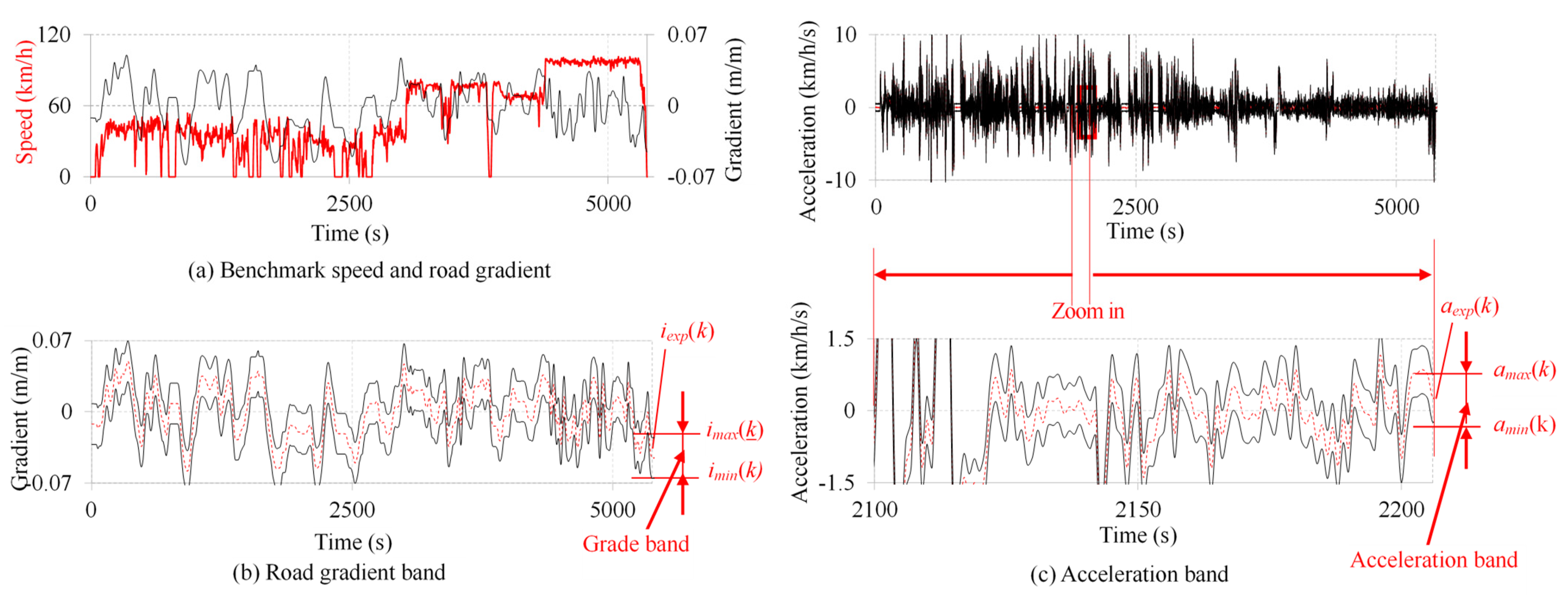
where Δa and Δi are the change bandwidths for the acceleration and road gradient actions, respectively; aexp(k) and iexp(k) are the acceleration and road gradient actions at time step k in the RDE test, respectively. Figure 2 shows the action control domain guided by the vehicle acceleration and terrain gradient of the benchmark RDE test. In the figure, Δa is set to 0.5 km/h/s, and Δi is set to 0.02 m/m.
The benchmark RDE test was selected from an RDE test conducted in the city district of Chongqing. The RDE test route has been certified and registered by the Chinese Ministry of Ecology and Environment. The section composition and terrain topography of the test route comply with the requirements of the RDE test procedure, and the traffic conditions on the test route are also suitable for the driver’s operation to satisfy the trip dynamics required by the RDE test procedure. Using the trip dynamics of the RDE test as a guide, the acceleration characteristics of the constructed driving cycles can be adjusted to approximate those of human drivers, thereby avoiding unrealistic operating behaviors, such as frequent and violent acceleration and braking actions. Similarly, using the road gradient from the RDE test as a guide in the gradient action optimization, the real-world road gradient and its continuous change characteristics can be emphasized, thereby avoiding sudden steps and potholes on the driving road that may arise in gradient action optimization. In addition, since the benchmark RDE test complies with all requirements of the RDE test procedure, minor changes in acceleration and gradient actions are unlikely to cause the trip dynamics and road terrain in the optimal solution to exceed the scope permitted by the RDE test procedure.

2.3. DP Algorithm

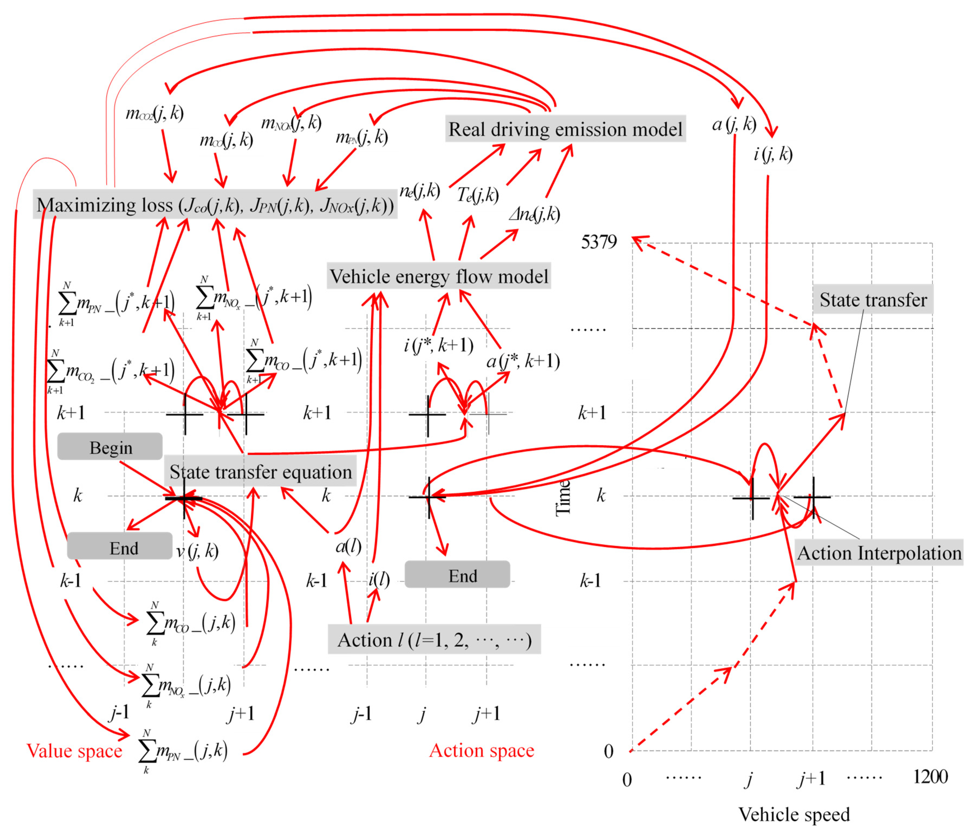
The benchmark RDE test was discretized into a series of time grids with a time step of 1 s and a total duration of 5379 s. Referring to the route composition of the benchmark RDE test, the period from 0 to 3050 s was set to be the urban trip section, the period from 3051 to 4393 s was set to be the rural trip section, and the period from 4394 to 5379 s was set to be the motorway trip section. To facilitate the state and action optimization, the vehicle speed was discretized at a resolution of 0.1 km/h. Additionally, the action space was finely discretized: acceleration actions were discretized with a step size of 0.02 km/h/s, while road gradient actions were discretized with a step size of 0.0005 m/m. Based on the Bellman optimization decision principle, A DP algorithm was developed to solve the multi-stage decision optimization model, which includes a backward and a forward solution process [30].
The DP backward solution algorithm sets the value loss of the Nth time step to zero, then step by step calculates the value loss of all states at each time step starting from the (N − 1)th time step, searching for the action strategy within the action control domain so that the value loss is maximized. For the jth state in the kth time step, there must exist an optimal action strategy in the action control domain that maximizes the value loss of the multi-stage decision with the kth time step as the initial stage and the jth state as the initial state:
J C O j , k = max k N m C O _ j , k k N m C O 2 _ j , k × M W L T C , C O 2
J P N j , k = max k N m P N _ j , k k N m C O 2 _ j , k × M W L T C , C O 2
J N O x j , k = max k N m N O x _ j , k k N m C O 2 _ j , k × M W L T C , C O 2
where JCO(j, k), JPN(j, k), and JNOx(j, k) are the value loss functions for CO, PN, and NOx emissions at the (j, k) grid node, respectively; k N m C O _ ( j , k ) , k N m P N _ ( j , k ) , k N m N O x _ ( j , k ) , k N m C O 2 _ ( j , k ) represent the cumulative CO, PN, NOx, and CO2 emissions from the kth time step and the jth state to the Nth time step:
k N m C O _ j , k = m C O j , k + k + 1 N m C O _ j , k + 1
k N m P N _ j , k = m P N j , k + k + 1 N m P N _ j , k + 1
k N m N O x _ j , k = m N O x j , k + k + 1 N m N O x _ j , k + 1
k N m C O 2 _ j , k = m C O 2 j , k + k + 1 N m C O 2 _ j , k + 1
where mCO(j, k), mPN(j, k), mNOx(j, k), mCO2(j, k) represent the transient CO, PN, NOx, and CO2 emissions due to the selected action at (j, k) grid node; k + 1 N m C O _ ( j , k + 1 ) , k + 1 N m P N _ ( j , k + 1 ) , k + 1 N m N O x _ ( j , k + 1 ) , k + 1 N m C O 2 _ ( j , k + 1 ) represent the cumulative CO, PN, NOx, and CO2 emissions from the stage (k + 1)th and the state j*th to the final stage Nth; j* denotes the state coordinate at the stage (k + 1)th due to the action selected at the grid node (j, k), which is determined by the state transition equation. The state transition equation indicates the state transition at the (k + 1)th time step caused by the selected acceleration action on the state at the (j, k) grid node:
v j , k + 1 = v j , k + a j , k
where v(j*, k + 1) denotes the vehicle speed at the next time step due to the action strategy a(j, k) at the (j, k) grid node. v(j*, k + 1) obtained by Equation (24) can be used to interpolate the coordinate position of j* on the state coordinate axis. If v(j*, k + 1) calculated using Equation (24) under the selected action exceeds the predetermined vehicle speed limit, the action should be excluded from the optimization process. After determining the coordinates of j*, the DP backward solution algorithm can obtain k + 1 N m C O _ ( j , k + 1 ) , k + 1 N m P N _ ( j , k + 1 ) , k + 1 N m N O x _ ( j , k + 1 ) , and k + 1 N m C O 2 _ ( j , k + 1 ) in the (k + 1)th time step through linear interpolation of neighboring grids, thereby calculating the value loss at the (j, k) grid node, as shown in Figure 3.
In the multi-stage decision process, calculating the maximum value loss at the (j, k) grid node requires determining the pollutant emissions under all the discretized actions in the action control space. For the lth action at the (j, k) grid node, the engine operating parameters (i.e., speed and torque) can be calculated by the state (vehicle speed) and action (acceleration and terrain gradient) at the state-time grid node based on the vehicle energy flow model. Then, the real driving emission model can calculate the transient CO, PN, NOx, and CO2 emissions at the (j, k) grid node, which are mCO(j, k), mPN(j, k), mNOx(j, k), and mCO2(j, k) in Equations (20)–(23). As mentioned above, if the lth action causes an engine start-stop event, the pollutant emissions generated by the action selection will be adjusted by adding a start-stop emission amount. The determination of engine start-stop events is based on engine speed and the rate of change in speed. The engine speed change rate is:
Δ n e j , k = n e j , k + 1 n e j , k
where Δne(j, k) is the change rate in engine speed at the grid node (j, k); ne(j, k) is the engine speed at the grid node (j, k); and ne(j*, k + 1) is the engine speed at the grid node (j*, k + 1), which is calculated by interpolating the engine speed data stored at adjacent points [31]. ne(j, k) and ne(j*, k + 1) can also be calculated using the state (vehicle speed) and action (acceleration and terrain gradient) at the respective state-time grid node. When Δne(j, k) is greater than the threshold value and ne(j, k) is zero, an engine start-stop event is identified. Then, Equations (17)–(23) can be used to calculate the value loss at the current time step, current state, and current action. Next, the DP backward solution algorithm selects another action from the action control domain, then repeats the above process until the value losses have been calculated for all possible actions in the action control domain at the (j, k) grid node. Then, the action that causes the most significant value loss at the (j, k) grid node can be identified in the action control domain. Accordingly, k N m C O _ ( j , k ) , k N m P N _ ( j , k ) , k N m N O x _ ( j , k ) , and k N m C O 2 _ ( j , k ) under the optimal action, as well as the optimal actions denoted as a(j, k) and i(j, k), are stored in the (j, k) grid node. Then, the optimization process at the current grid node is terminated. The action optimization process at the (j, k) grid node during the DP backward solution is illustrated in Figure 3.
Subsequently, the action optimization continues for the next grid node in the kth time step until the action optimization at 1201 grid nodes in the kth time step is completed. Then, the above action optimization process is repeated at the (k − 1)th, (k − 2)th, … time steps until the action optimization has been conducted for all the 1201 × 5379 state-time grid nodes. Next, the DP forward solution proceeds. Starting from the initial state (vehicle speed), the DP forward solution algorithm interpolates the optimal action (acceleration and slope) from the optimal action strategies stored in the state-time grid nodes, then obtains the state at the next time step using the state transition equation. Based on the state at the next time step, the DP forward solution algorithm interpolates the optimal action at the next time step from the action strategies stored in the state grid at the next time step, then uses the state transition equation to obtain the state at the second-next time step. In the forward step-by-step process, the DP forward solution algorithm completes the calculation of states and actions at all the time steps in the time control domain by alternating action interpolation and state transitions, as shown in Figure 3. The resulting status (vehicle speed) and actions (acceleration and terrain gradient) constitute the emission-intensive driving cycles for emission testing. The DP algorithm’s logic is shown in Algorithm 1. This DP algorithm was implemented using MATLAB programming. The computation time for the algorithm to generate one driving cycle was approximately 11,881 s (about 3 h and 20 min), running on a workstation equipped with an Intel Core i7-8750H processor and 16 GB of DDR4 memory.
Algorithm 1. DP algorithm for Generating High-Emission Driving Cycle
Input: vehicle parameters, time step Δt, total stages N, baseline speed vexp(k), acceleration aexp(k), road grade iexp(k), real driving emission model.
1  Initialize grids of speed v ∈ [vmin, vmax], acceleration a, and road grade i.
2  for k = N − 1 to 1 do
3    for each discrete speed v do
4      for each action [a, i] around baseline do
5        Compute next speed vnext = v + a·Δt
6        Compute demanded power Pdem = f(v, a, i)
7        Map Pdemne, Te → current emissions (CO2, CO, PN, NOx)
8        Compute cumulative emissions: current emissions + future optimal emissions (from the value matrix at vnext)
9        Evaluate emission metric J(v, a, i)
10      end
11      Select (a*, i*) = arg max J(v, a, i)
12    end
13  end
14  Forward simulate with policy [a*(k), i*(k)] to generate cycle
Output: optimized action sequence [a*(k), i*(k)] and the corresponding high-emission driving cycle.

3. Results and Discussions

3.1. Characteristics of Emission-Intensive Driving Cycles

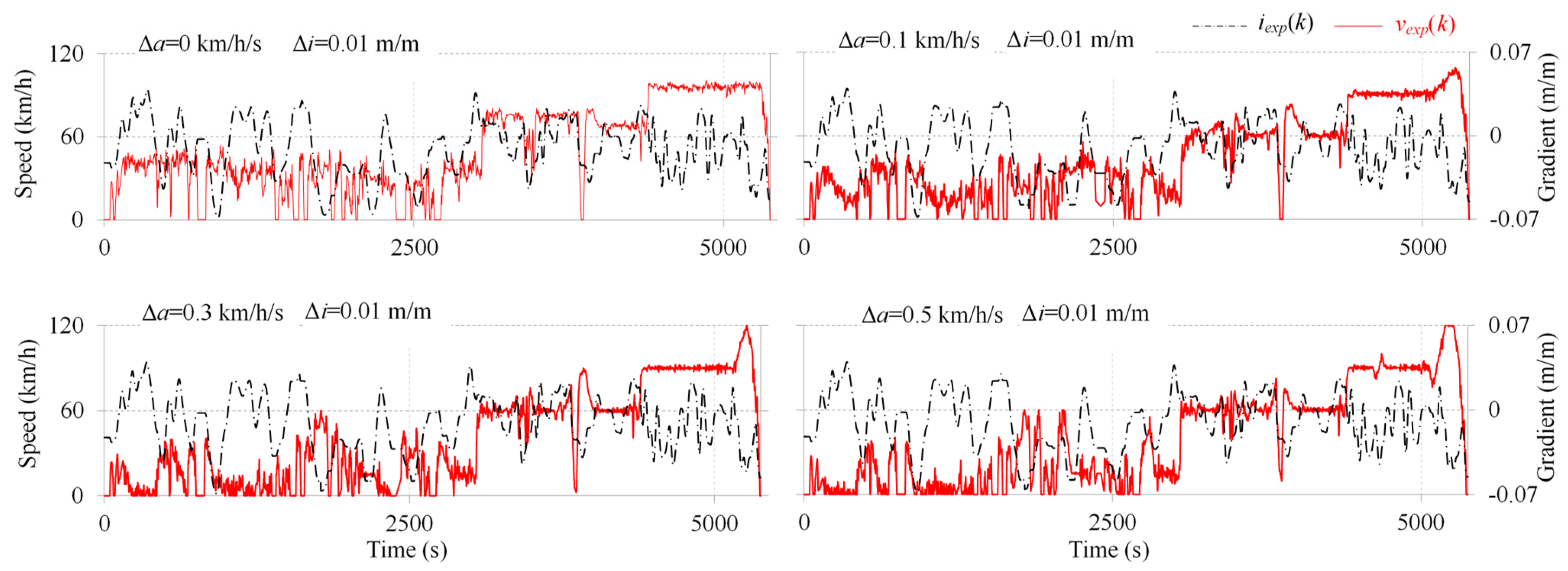
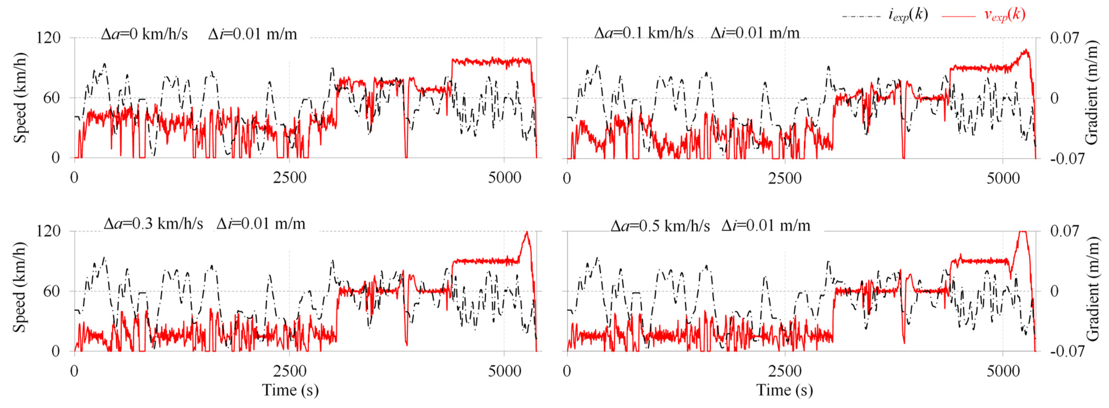
Figure 4 shows the constructed driving cycles targeting CO emissions with the acceleration adjustment bandwidths of 0, ±0.1, ±0.3, and ±0.5 km/h/s, respectively, and the gradient adjustment bandwidth of ±0.01 m/m. In the urban section, the vehicle drives at approximately 40 km/h, with occasional stops, when the acceleration adjustment bandwidth is set to zero. As the acceleration adjustment bandwidth increases, the vehicle tends to drive around the upper limit speed of 60 km/h or the near-zero low speed. When the acceleration adjustment bandwidth increases to ±0.5 km/h/s, high-frequency events alternating between low-speed driving, stopping, and restarting can be observed, resembling driving conditions in congested urban traffic. In the rural section, the vehicle drives at about 80 km/h when the acceleration adjustment bandwidth is set to zero. As the acceleration adjustment bandwidth increases, the vehicle tends to drive closer to the lower speed limit of 60 km/h. Still, there are also instances where the vehicle accelerates to the upper limit of 90 km/h. In the motorway section, the vehicle speed maintains a relatively constant approximately 95 km/h when the acceleration adjustment bandwidth is set to zero. After increasing the acceleration adjustment bandwidth, the vehicle drives at a speed close to the lower limit of 90 km/h in the latter part of the trip section, then gradually accelerates to the upper limit of 120 km/h. As can be seen, the DP algorithm tends to control the vehicle at the lower limit speed and adopts high-frequency but low-intensity acceleration and deceleration actions to worsen CO emissions. Secondly, acceleration to the upper speed limit can also be occasionally observed, indicating that aggressive driving behavior affects pollutant emissions to some degree. In addition, comparing the terrain profile in the benchmark RDE test and that in the constructed driving cycle with the acceleration adjustment bandwidths of zero, it is found that the latter selects the actions closer to the lower limit of the gradient adjustment bandwidth. The DP algorithm tends to utilize the lower bounds in the action control domain, potentially relating to the CO2 emission corrections involved in the pollutant emission normalization method specified in the RDE test procedure (see Equations (7)–(9)).
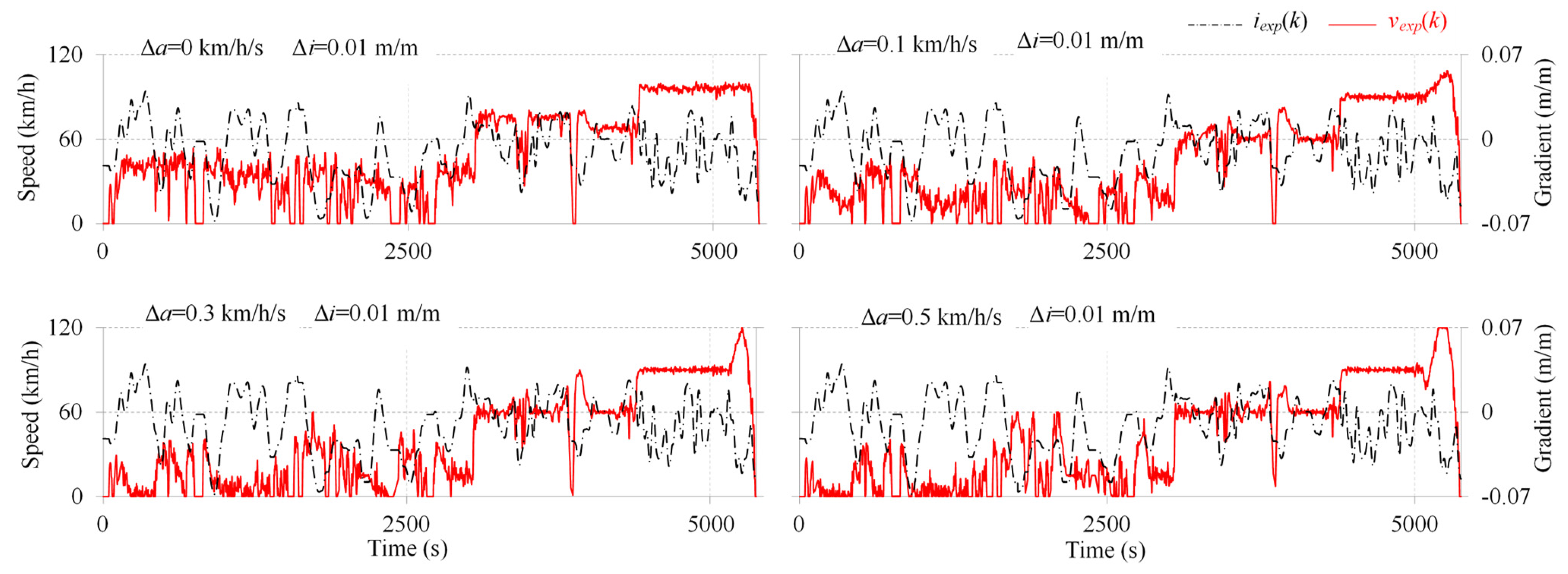
CO and PN emissions both originate from the localized enrichment of the in-cylinder mixture and are similarly affected by engine start-stop events. Thus, the DP solutions targeting PN emissions are very close to those targeting CO emissions, as shown in Figure 5. However, NOx emissions differ from CO and PN emissions in the in-cylinder formation mechanism and are primarily affected by engine start-stop events only during motorway driving conditions. Therefore, the constructed driving cycles targeting NOx emissions differ from those targeting CO and PN emissions. Figure 6 shows the constructed driving cycles targeting NOx emissions. In the urban section, when the acceleration adjustment bandwidth is set to ±0.5 km/h/s, the constructed driving cycle will be centered on a speed of 20 km/h, allowing for moderate acceleration and deceleration around that speed. Overall, the vehicle speed remains relatively stable throughout the urban section and does not exhibit the frequent stopping, acceleration, and deceleration as those seen in constructed driving cycles targeting CO and PN emissions. In the rural section, the vehicle still mainly adheres to the lower limit of 60 km/h. In the motorway section, the constructed driving cycle targeting NOx emissions tends to drive the vehicle near the lower limit speed of 90 km/h and accelerate it to the upper limit speed of 120 km/h in the latter part of the trip section.
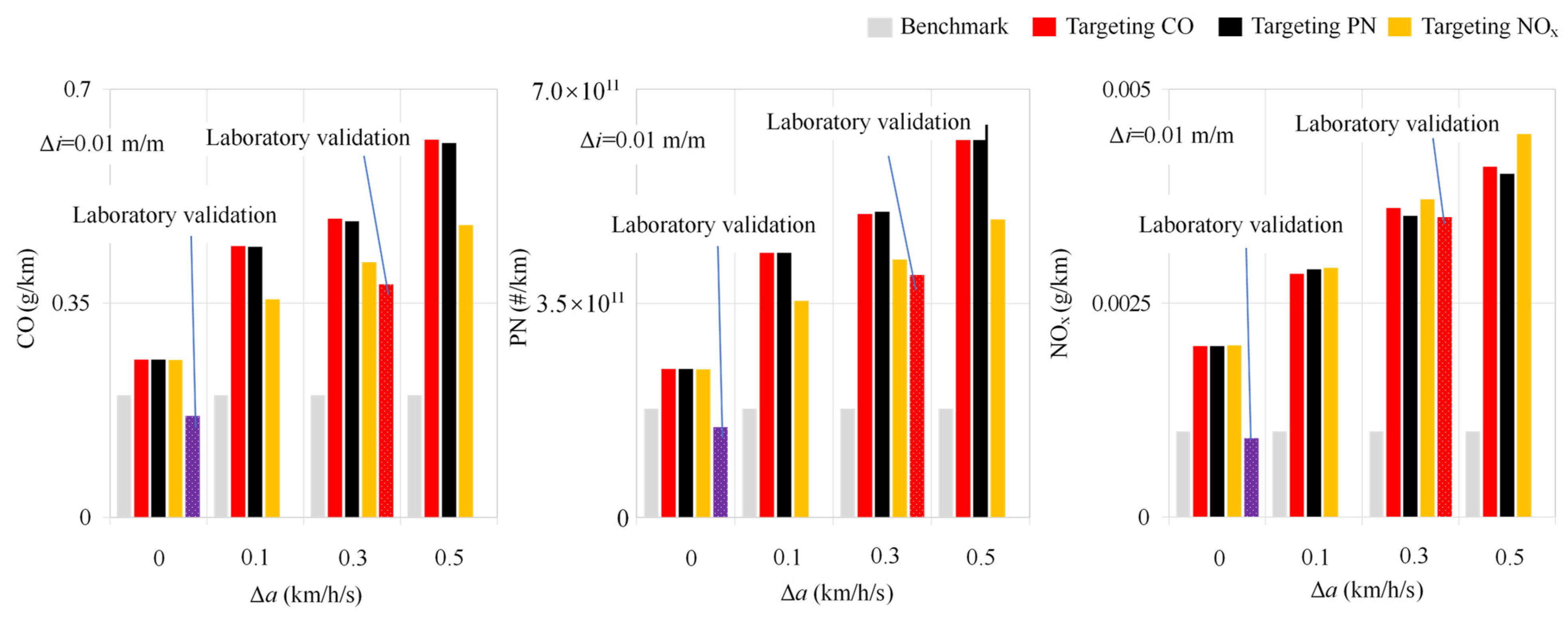
Figure 7 shows the specific-distance emissions generated by the DP algorithm for the 12 driving cycles and the benchmark RDE test cycle. When the acceleration adjustment bandwidth increases to ±0.5 km/h/s, the specific-distance CO emissions of the constructed driving cycles targeting CO emissions increase to 0.617 g/km, the specific-distance PN emissions increase to 6.372 × 10¹¹ #/km, and the specific-distance NOx emissions increase to 0.00409 g/km, which are 3.09, 3.59, and 4.08 times those of the benchmark RDE test, respectively. The constructed driving cycles targeting PN emissions are almost the same as those targeting PN emissions in terms of the specific-distance emissions. However, the constructed driving cycles targeting NOx emissions enable higher specific-distance NOx emissions, but lower specific-distance CO and PN emissions, whose specific-distance CO, PN, and NOx emissions are 2.40, 2.74, and 4.46 times of the benchmark RDE test, respectively. It can be seen that the constructed driving cycles have significantly stringent emission characteristics. Additionally, road terrain optimization is essential for constructing emission-intensive driving cycles. When the acceleration adjustment bandwidth is set to zero and the gradient adjustment bandwidth is set to ±0.01 m/m, the CO emissions generated by the constructed driving cycle increase to approximately 1.30 times that of the benchmark RDE test, the PN emissions increase to approximately 1.37 times, and the NOx emissions increase to approximately 1.99 times. At the same time, the gradient adjustment does not significantly alter the cumulative positive altitude gain of the constructed driving cycle. For example, when Δa is 0.5 km/h/s, the cumulative positive altitude gains of the constructed driving cycle targeting CO, PN, and NOx emissions are, respectively, 610 m/100 km, 606 m/100, and 547 m/100 km, which are significantly lower than the regulatory limit of 1200 m/100 km. The DP algorithm does not consistently pursue steep gradients, likely due to CO2 normalization in emission calculations. While steeper gradients increase CO, PN, and NOx emissions, they also sensitively elevate CO2 emissions. Thus, the DP algorithm strikes a compromise between these two trends.

3.2. Verification of Emission-Intensive Driving Cycles

As mentioned earlier, this study directly uses the compliant trip dynamics and terrain characteristics of a benchmark RDE test as a guide to determine the acceleration and road gradient changes at each time step in the time control domain. Consequently, the limited adjustments in acceleration and gradient actions are less likely to cause the speed profiles in the optimal solutions to exceed the scope permitted by the RDE test procedure. As shown in Figure 4, when Δa is 0.5 km/h/s, the average speeds for the urban, rural, and motorway trips of the stringent CO emission target driving cycle are 27.77 km/h, 72.17 km/h, and 98.25 km/h, respectively; urban stopping time accounts for 23.99%. Figure 5 shows that for the emission-intensive driving cycle targeting PN emissions when Δa is 0.5 km/h/s, the average speeds for urban, rural, and motorway trips are 28.19 km/h, 72.95 km/h, and 98.07 km/h, respectively; urban stopping time accounts for 24.08%. Figure 6 shows the emission-intensive driving cycle targeting NOx emissions when Δa is 0.5 km/h/s, with average speeds of 23.35 km/h, 72.30 km/h, and 98.09 km/h for urban, rural, and motorway trips, respectively; urban stop time accounted for 9.67%. It is evident that the average speeds across all road sections and the proportion of urban stop time fully comply with the requirements of the RDE regulation procedure. Under conditions of narrower acceleration adjustment bandwidth (Δa is 0.1 or 0.3 km/h/s), the aforementioned compliance of the generated driving cycles would be even more assured.
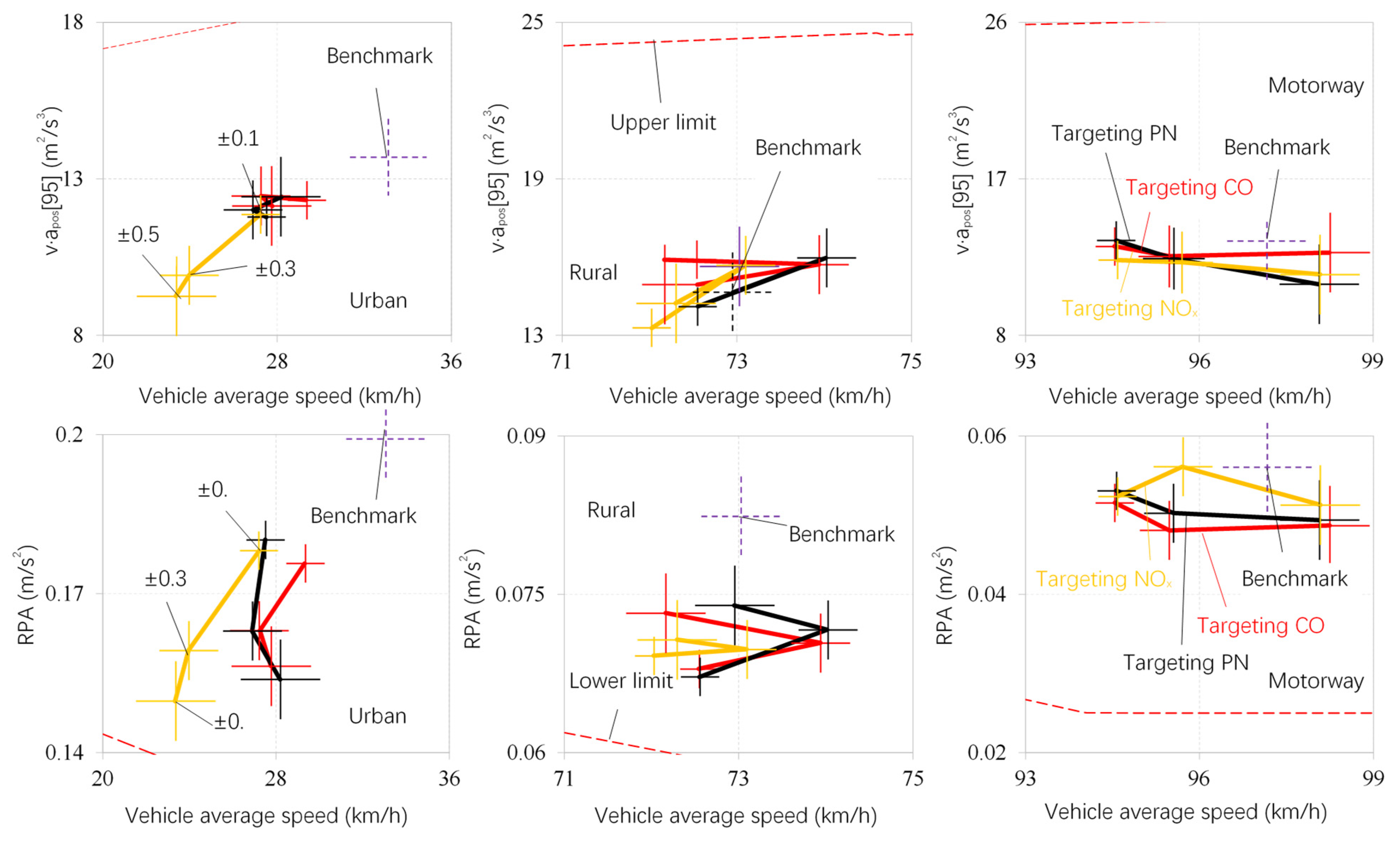
Figure 8 shows the trip dynamics verification for the constructed 12 driving cycles and the benchmark RDE test. Currently, v·apos [95] (the 95th percentile of the product of the vehicle speed and positive acceleration greater than 0.1 m/s2) and related positive acceleration (RPA) are used to characterize the trip dynamics in the RDE test procedure.
In the figure, the case of the constructed driving cycles with the acceleration control bandwidth of zero is identical to the case of the benchmark RDE test. As can be seen, none of the constructed driving cycles exhibits excessive or insufficient trip dynamics characteristics. v·apos [95] of each road section in the constructed driving cycle is almost lower than that under the benchmark RDE test, showing a downward trend with increasing the acceleration control bandwidth in most cases. There is no evidence to suggest that increasing the acceleration adjustment bandwidth will result in more aggressive trip dynamics in the constructed driving cycles. In addition, the RPA of each road section in the constructed driving cycles is above the regulatory lower limit and lower than that of the benchmark RDE test. As the acceleration adjustment bandwidth increases, the RPA exhibits a slight downward trend, thereby increasing the risk of insufficient dynamic characteristics in the constructed driving cycles. Although the vehicle accelerates to 120 km/h in the later stage of the motorway section can be observed, the overall aggressive trip dynamics of the constructed driving cycle are not exhibited. The DP-based strategy for constructing emission-intensive driving cycles of the extended-range electric vehicle is inconsistent with those widely favored in existing research, which tends to worsen pollutant emissions by aggressive trip dynamics.
To verify the feasibility and effectiveness of reproducing the constructed emission-intensive driving cycles under laboratory conditions, emissions testing was conducted at a chassis dynamometer using the benchmark RDE test driving cycle and the emission-intensive driving cycle targeting CO emissions with the acceleration adjustment bandwidth of ±0.3 km/h/s. As shown in Figure 7, the PN and NOx emission factors generated under their emission-intensive driving cycle are well below the regulatory NTE limits, indicating a substantial margin for compliance. In contrast, CO emissions present a certain compliance risk, making the emission-intensive driving cycle targeting CO emissions a priority concern. During the tests, road gradient resistance was included as part of road driving resistance in the simulated loading. The specific-distance pollutant emissions under the benchmark RDE test driving cycle and the emission-intensive driving cycle are also presented in Figure 7, which are compared with those obtained using the DP algorithm. As can be seen, the specific-distance NOx emissions resulting from running the emission-intensive driving cycle targeting CO emissions on the chassis dynamometer do not differ significantly from those given by the DP algorithm, but the specific-distance CO and PN emissions are about 20% lower than those provided by the DP algorithm. The reason may lie in the fact that the constructed real driving emissions model over-measures the effect of engine start-stop on pollutant emissions, or the driver cannot follow the target speed profile exactly on the chassis dynamometer, causing the actual speed profile to deviate from the constructed emission-intensive driving cycle. However, in any case, the severe emission properties of the emission-intensive driving cycles given by the DP algorithm can be verified on the laboratory chassis dynamometer.

4. Conclusions

The DP approach builds the value function using the normalized specific-distance pollutant emissions, treats vehicle speed and road gradient as actions, and searches for the optimal actions within the possible action domain to maximize the value loss over the vehicle’s driving cycle. Utilizing the DP approach, the problem of constructing an emission-intensive driving cycle can be transformed into a multi-stage decision optimization problem in a time control domain. Assembling the real driving emission model and the multi-stage decision optimization model, the DP algorithm is proven to efficiently generate severe emission driving scenarios in the action control domain, thus enabling the construction of emissions-intensive driving cycles.
The RDE test procedure imposes complicated restrictions on trip dynamics and road terrain that cannot be used directly to outline the action control domain in the multi-stage decision optimization model. In this regard, the trip dynamics and road terrain of a benchmark RDE test were used as guidance to carve out the action control domains. This ensures the trip dynamics of the constructed driving cycle align with the operating styles of human drivers and also avoids unrealistic road terrain in the solution of the DP problem. Introducing the benchmark RDE test to aid in defining the action domain and time control domain in the DP approach is efficient in keeping the multi-stage decision optimization compliant with the RDE regulatory test boundary conditions.
The DP algorithm tends to construct emission-intensive driving cycles using high-frequency, low-intensity acceleration and deceleration actions, in addition to violently aggressive driving, which is generally considered to be most closely related to severe emissions. The decoupling of engine speed from vehicle speed and the significant impact of engine start-stop on emissions determine the unique characteristics of pollutant emissions from range-extended electric vehicles. Additionally, the effect of road terrain on real driving emissions should not be overlooked. Introducing coordinated optimization between trip dynamics and road terrain into the construction of emission-intensive driving cycles can more realistically reproduce the severe emissions scenarios encountered during real-world driving.
However, this study is currently limited to a single vehicle operating in charge-sustaining mode, with an action space guided by a single route and a lack of extensive experimental validation. Future research should therefore aim to validate the approach across a wider variety of vehicle types and more diverse action bandwidths. It should also incorporate more emission data from laboratory chassis dynamometer tests to verify the algorithm’s accuracy and general applicability. Additionally, further refinement is needed to guide the DP algorithm toward better approximating human driving behavior and to prevent it from selecting abnormal terrain (e.g., unrealistically steep gradients). These will enhance the practical relevance and applicability of the constructed emission-intensive driving cycles for RDE calibration.

Author Contributions

Conceptualization, L.Z. and Q.Z.; methodology, Y.C. and L.Z.; software, Y.C., H.X. and C.J.; validation, Y.C., H.X. and Q.Z.; formal analysis, Y.C., H.X. and C.J.; investigation, Y.C., H.X. and Q.Z.; resources, L.Z. and Q.Z.; data curation, Y.C., H.X. and C.J.; writing—original draft preparation, Y.C.; writing—review and editing, L.Z.; visualization, Y.C., H.X. and C.J.; supervision, L.Z. and Q.Z.; project administration, L.Z.; funding acquisition, L.Z. All authors have read and agreed to the published version of the manuscript.

Funding

This research was funded by the Chongqing Technology Innovation and Application Development Project (Grant Numbers: CSTB2022TIAD–KPX0139 and CSTB2022TIAD-KPX0050), the Chongqing research institution performance incentive guidance special program (Grant Number: CSTB2023JXJL–YFX0037), and the Natural Science Foundation of Chongqing (Grant Numbers: CSTB2022NSCQ-MSX1359).

Institutional Review Board Statement

Not applicable.

Informed Consent Statement

Not applicable.

Data Availability Statement

The data presented in this study are available on request from the corresponding author. The data are not publicly available due to the protection of data privacy and intellectual property rights.

Conflicts of Interest

Author Qing Zhang was employed by the company Chongqing Changan Automobile Co., Ltd. The remaining authors declare that the research was conducted in the absence of any commercial or financial relationships that could be construed as a potential conflict of interest.

References

  1. Hooftman, N.; Messagie, M.; Van Mierlo, J.; Coosemans, T. A review of the European passenger car regulations-Real driving emissions vs local air quality. Renew. Sustain. Energy Rev. 2018, 86, 1–21. [Google Scholar] [CrossRef]
  2. Ribeiro, C.B.; Rodella, F.H.C.; Hoinaski, L. Regulating light-duty vehicle emissions: An overview of US, EU, China and Brazil programs and its effect on air quality. Clean Technol. Environ. 2021, 24, 851–862. [Google Scholar] [CrossRef] [PubMed]
  3. Wallington, T.J.; Anderson, J.E.; Dolan, R.H.; Winkler, S.L. Vehicle emissions and urban air quality: 60 years of progress. Atmosphere 2022, 13, 650. [Google Scholar] [CrossRef]
  4. Tutuianu, M.; Bonnel, P.; Ciuffo, B.; Haniu, T.; Ichikawa, N.; Marotta, A.; Pavlovic, J.; Steven, H. Development of the world-wide harmonized light duty test cycle (WLTC) and a possible pathway for its introduction in the European legislation. Transp. Res. Part D Transp. Environ. 2015, 40, 61–75. [Google Scholar] [CrossRef]
  5. Bishop, J.D.K.; Axon, C.J. Using natural driving experiments and Markov chains to develop realistic driving cycles. Transp. Res. Part D Transp. Environ. 2024, 137, 104507. [Google Scholar] [CrossRef]
  6. Liu, G.F.; Yang, X.H.; Pei, B.; Xu, H.M.; Wu, B.Y.; Su, W.H. Development of a representative transient cycle for evaluating real driving emissions of heavy-duty diesel engines. Atmos. Pollut. Res. 2025, 16, 102520. [Google Scholar] [CrossRef]
  7. Cui, Y.P.; Zou, F.M.; Xu, H.; Chen, Z.H.; Gong, K.M. A novel optimization-based method to develop representative driving cycle in various driving conditions. Energy 2022, 247, 123455. [Google Scholar] [CrossRef]
  8. Huzayyin, O.A.; Salem, H.; Hassan, M.A. A representative urban driving cycle for passenger vehicles to estimate fuel consumption and emission rates under real-world driving conditions. Urban Clim. 2021, 36, 100810. [Google Scholar] [CrossRef]
  9. Yang, D.P.; Liu, T.; Zhang, X.M.; Zeng, X.H.; Song, D.F. Construction of high-precision driving cycle based on Metropolis-Hastings sampling and genetic algorithm. Transp. Res. Part D Transp. Environ. 2023, 118, 103715. [Google Scholar] [CrossRef]
  10. Rahman, S.M.A.; Fattah, I.M.R.; Ong, H.C.; Ashik, F.R.; Hassan, M.M.; Murshed, M.T.; Imran, M.A.; Rahman, M.H.; Rahman, M.A.; Hasan, M.A.; et al. State-of-the-art of establishing test procedures for real driving gaseous emissions from light- and heavy-duty vehicles. Energies 2021, 14, 4195. [Google Scholar] [CrossRef]
  11. EC. Commission Regulation (EU) 2016/646 of 20 April 2016 amending Regulation (EC) No 692/2008 as regards emissions from light passenger and commercial vehicles (Euro 6). Off. J. Eur. Union 2016, L 109, 1. [Google Scholar]
  12. Varella, R.A.; Faria, M.V.; Mendoza-Villafuerte, P.; Baptista, P.C.; Sousa, L.; Duarte, D.O. Assessing the influence of boundary conditions, driving behavior and data analysis methods on real driving CO2 and NOx emissions. Sci. Total Environ. 2019, 658, 879–894. [Google Scholar] [CrossRef] [PubMed]
  13. Shahariar, G.M.H.; Bodisco, T.A.; Zare, A.; Sajjad, M.; Jahirul, M.I.; Van, T.C.; Bartlett, H.; Ristovski, Z.; Brown, R.J. Impact of driving style and traffic condition on emissions and fuel consumption during real-world transient operation. Fuel 2022, 319, 123874. [Google Scholar] [CrossRef]
  14. Jiang, Z.W.; Niu, H.M.; Jia, Z.Y.; Wu, L.; Zhang, Q.J.; Zhang, Y.J.; Mao, H.J. Comparison of vehicular emissions at different altitudes: Characteristics and policy implications. Environ. Pollut. 2025, 367, 125679. [Google Scholar] [CrossRef]
  15. Du, B.C.; Zhang, L.; Geng, Y.T.; Zhang, Y.; Xu, H.L.; Xiang, G. Testing and evaluation of cold-start emissions in a real driving emissions test. Transp. Res. Part D Transp. Environ. 2020, 86, 102447. [Google Scholar] [CrossRef]
  16. Xu, H.L.; Zhang, L.; Chang, H.; Han, J.L.; Wu, D.M.; Gong, X.K.; Fu, M.M. Measuring the route topography impact on real driving emissions based on neural network models. Environ. Res. 2023, 231, 116072. [Google Scholar] [CrossRef]
  17. Classen, J.; Pischinger, S.; Krysmon, S.; Sterlepper, S.; Dorscheidt, F.; Doucet, M.; Reuber, C.; Gorgen, M.; Scharf, J.; Nijs, M.; et al. Statistically supported real driving emission calibration: Using cycle generation to provide vehicle-specific and statistically representative test scenarios for Euro 7. Int. J. Engine Res. 2020, 21, 1783–1799. [Google Scholar] [CrossRef]
  18. Krysmon, S.; Classen, J.; Pischinger, S.; Trendafilov, G.; Duezguen, M.; Dorscheidt, F. RDE calibration-evaluating fundamentals of clustering approaches to support the calibration process. Vehicles 2023, 5, 404–423. [Google Scholar] [CrossRef]
  19. Lee, S.Y.; Andert, J.; Neumann, J.; Querel, C.; Scheel, T.; Aktas, S.; Ehrly, M.; Schaub, J.; Kotter, M. Hardware-in-the-loop-based virtual calibration approach to meet real driving emissions requirements. SAE Int. J. Engines 2018, 11, 1479–1504. [Google Scholar] [CrossRef]
  20. Classen, J.; Krysmon, S.; Dorscheidt, F.; Sterlepper, S.; Pischinger, S. Real driving emission calibration-review of current validation methods against the background of future emission legislation. Appl. Sci. 2021, 11, 5429. [Google Scholar] [CrossRef]
  21. Wasserburger, A.; Didcock, N.; Hametner, C. Efficient real driving emissions calibration of automotive powertrains under operating uncertainties. Eng. Optim. 2023, 55, 140–157. [Google Scholar] [CrossRef]
  22. Hu, R.; Zhang, F.; Peng, Z.J.; Pei, Y.Q. The NOx emission characteristics of gasoline vehicles during transient driving cycles. Transp. Res. Part D Transp. Environ. 2022, 109, 103386. [Google Scholar] [CrossRef]
  23. Guo, D.D.; Ge, Y.S.; Wang, X.; Liu, H.X.; Su, S.; Li, C.B.; Tao, T.H. Evaluating the filtration efficiency of close-coupled catalyzed gasoline particulate filter (cGPF) over the WLTC and simulated RDE cycles. Chemosphere 2022, 301, 134717. [Google Scholar] [CrossRef] [PubMed]
  24. Fernandes, P.; Tomas, R.; Ferreira, E.; Bahmankhah, B.; Coelho, M.C. Driving aggressiveness in hybrid electric vehicles: Assessing the impact of driving volatility on emission rates. Appl. Energy 2021, 284, 116250. [Google Scholar] [CrossRef]
  25. Du, B.C.; Zhang, L.; Zou, J.; Han, J.L.; Zhang, Y.; Xu, H.L. Investigating the impact of route topography on real driving emission tests based on large data sample at data window level. Sci. Total Environ. 2022, 809, 151133. [Google Scholar] [CrossRef]
  26. GB18352.6-2016; Limits and Measurement Methods for Emissions from Light-Duty Vehicles. China Environmental Science Press: Beijing, China, 2016.
  27. Xu, H.L.; Chen, Y.; Zhang, L.; Chen, G.L.; Han, J.L.; Zhang, Q.; Li, C.K. Energy management strategies for extended-range electric vehicles with real driving emission constraints. Appl. Sci. 2025, 15, 142. [Google Scholar] [CrossRef]
  28. Giakoumis, E.G.; Alafouzos, A.I. Study of diesel engine performance and emissions during a Transient Cycle applying an engine mapping-based methodology. Appl. Energy 2010, 87, 1358–1365. [Google Scholar] [CrossRef]
  29. Mantz, H.; Jacobs, K.; Mecke, K. Utilizing Minkowski functionals for image analysis: A marching square algorithm. J. Stat. Mech. Theory Exp. 2008, 12, 12015. [Google Scholar] [CrossRef]
  30. Bellman, R.E.; Dreyfus, S.E. Applied Dynamic Programming; Princeton University Press: Princeton, NJ, USA, 1962. [Google Scholar]
  31. Wang, Y.Z.; Zhang, L.; Chen, Y.; Li, C.K.; Du, B.C.; Han, J.L. Energy management strategies for hybrid diesel vehicles by dynamic planning embedded in real-world driving emission model. Case Stud. Therm. Eng. 2025, 65, 105643. [Google Scholar] [CrossRef]
Figure 1. Performance of the real-world driving emission model taking into account engine start-stop emissions.
Applsci 15 11762 g001
Figure 2. Action adjustment bandwidths guided by the trip dynamic and road gradient of the benchmark RDE test.
Applsci 15 11762 g002
Figure 3. Action optimization in the inverse solution process and optimal solution reconstruction in the forward solution process.
Applsci 15 11762 g003
Figure 4. Resulting emission-intensive driving cycles with CO emissions as the optimization target.
Applsci 15 11762 g004
Figure 5. Resulting emission-intensive driving cycles with PN emissions as the optimization target.
Applsci 15 11762 g005
Figure 6. Resulting emission-intensive driving cycles with NOx emissions as the optimization target.
Applsci 15 11762 g006
Figure 7. Specific-distance pollutant emissions of the extended-range electric passenger car under the resulting emission-intensive driving cycles.
Applsci 15 11762 g007
Figure 8. Trip dynamics verification for the emission-intensive driving cycles.
Applsci 15 11762 g008
Disclaimer/Publisher’s Note: The statements, opinions and data contained in all publications are solely those of the individual author(s) and contributor(s) and not of MDPI and/or the editor(s). MDPI and/or the editor(s) disclaim responsibility for any injury to people or property resulting from any ideas, methods, instructions or products referred to in the content.