Abstract
The current development in computer vision highlights the significance of comprehending the semantic features of images. However, the spatial front-back relationships between objects, which constitute a fundamental semantic feature, have received limited attention. To address this gap, we propose a novel neural network termed Spatial Front-Back Relationship Partition Sorting Network (SFBR-PSortNet), specifically designed for recognizing spatial front-back relationships among objects within images. SFBR-PSortNet is an end-to-end deep convolutional neural network that systematically generates a set of triples representing the spatial front-back relationships between every pair of objects in an input image. The key technical innovations of SFBR-PSortNet include the utilization of bottom keypoints of objects, which serve a dual purpose of enabling object category recognition and providing implicit depth information to enhance spatial front-back relationship reasoning, and the introduction of a Partition Sorting mechanism to construct a comprehensive spatial front-back relationship graph among all objects. Extensive experiments conducted on data derived from the KITTI dataset demonstrate the effectiveness of our network for spatial front-back relationship recognition, achieving a Precision of 0.876 and a Recall of 0.856, respectively. The results validate the practical applicability and robustness of our network in real-world road scenarios, underscoring its potential to enhance the accuracy of computer vision systems in complex environments.
1. Introduction
One of the most significant ongoing discussions in the field of computer vision revolves around object recognition and scene understanding, technologies that have found extensive applications in various domains such as security, medicine, and transportation. It involves the use of machines to process, analyze, and comprehend images based on their distinctive features (including texture, shape, and color patterns), enabling the identification of different objects and scenes with varying patterns. To achieve more profound understanding of the relationships among objects within an image, there is a growing trend towards extracting semantic relationships among objects during the recognition process. Among various spatial relationships, the spatial front-back relationship between objects emerges as a fundamental semantic feature, playing a crucial role in helping machines comprehend the positions, behaviors, and interactions of identified elements. Therefore, developing efficient methods for recognizing spatial front-back relationships holds considerable value, as this will significantly enhance scene understanding capabilities in computer vision systems. However, despite its fundamental importance, spatial front-back relationship detection has rarely been addressed as an independent and dedicated research focus, with existing approaches either incorporating it as a secondary component within broader visual understanding frameworks or deriving it indirectly from other primary tasks.
Over the past decade, the forefront of research within the field of computer vision has consistently been occupied by the development of image classification models and object detection models, both constructed with the framework of Convolutional Neural Networks (CNNs). As a prevalent deep learning architecture, CNNs originated in the 1990s, specifically with the work of [1], which formulated the LeNet-5 network for the classification of handwritten numerals based on the hierarchical processing mechanisms observed in the human visual cortex. Since 2012, a plethora of refined CNN architectures have emerged to address a diverse spectrum of visual tasks effectively. CNN-based classification models, ranging from AlexNet [2], VGGNet [3], GoogleNet [4], ResNet [5], DenseNet [6], to EfficientNet [7], have progressively improved, achieving remarkable accuracy rates that approach human-level performance on the ImageNet dataset by 2020. These models hierarchically extract features through convolution operations and transform them into classification results via pooling, fully connected, and softmax layers. Similarly, object detection algorithms based on CNNs have demonstrated excellent performance, with state-of-the-art models achieving mean Average Precision (mAP) scores of approximately 50% on the Microsoft Common Objects in Context (MS COCO) dataset as of 2022. Notable examples include the R-CNN [8] series, YOLO [9,10,11] series, CornerNet [12], and EfficientDet [13]. Modern detection algorithms generally employ a multi-stage structure: a backbone network for hierarchical feature extraction, a feature enhancement network for multi-scale information fusion, and a detection head that performs object classification and bounding box regression.
Although CNN-based recognition and detection methods have achieved remarkable success in visual tasks, these accomplishments are primarily confined to the low-level vision stage. An image typically consists of background and foreground elements, with the latter further categorized into various object classes, all of which coexist densely within a single image frame. Low-level vision methods often decouple these elements for recognition or detection purposes but tend to overlook the interrelationships among objects and their corresponding deeper semantic information. In contrast, spatial front-back relationships, as a representative form of mid-level vision, provide a more comprehensive understanding of scene layouts and positional relationships between objects. These relationships facilitate the perception of depth and distance among objects within a scene, thereby enhancing the overall comprehension of three-dimensional space. However, the attention this field has received is not commensurate with its importance.
Fortunately, in recent years, researchers have begun to explore methods that enable machines to perceive spatial front-back relationships between objects. This exploration primarily involves two key research directions: Visual Relationship Detection (VRD) [14] and depth estimation. VRD can be implemented through various computational frameworks including CNN-based approaches [15], graph-based spatial modeling [16], and transformer-based vision models [17]. Additionally, methods from related fields such as relational networks [18] (originally developed for visual reasoning) have also been adapted for VRD tasks. Spatial front-back relationship recognition represents a specialized category within VRD, focusing specifically on depth-aware spatial understanding between objects. Among the various computational frameworks for VRD, CNN-based approaches have shown particular promise for this task due to their ability to extract hierarchical depth-aware features. Consequently, many CNN-based VRD algorithms, such as those proposed by [19,20], incorporate front-back spatial features to enhance depth-aware perception in VRD. Building on this approach, Gan et al. [21] proposed an adaptive depth spatial location network which uses regional information variance to measure information relevance in each small region within an object bounding box, thereby generating a more accurate depth representation when locating object spatial front-back positions. Beyond the traditional CNN-based approaches, graph-based methods have emerged as another important paradigm for spatial relationship modeling. Graph Neural Networks (GNNs) represent objects as nodes and their spatial relationships as edges, enabling explicit modeling of complex spatial interactions through message passing and graph convolutions [22]. Similarly, relational networks and relation modules have been specifically designed to learn pairwise object relationships through dedicated architectural components [23]. In addition to these explicit relationship modeling approaches, recent advances in transformer-based vision models have also contributed to spatial reasoning capabilities. Chen et al. [24] propose an automatic three-dimensional (3D) spatial Visual Question Answering (VQA) data generation framework that creates 2 billion training examples to enhance vision language models’ spatial reasoning capabilities in both qualitative and quantitative tasks.
While these existing VRD approaches have made significant progress in general spatial reasoning, they share a common limitation: few are specifically designed to address the unique challenges of front-back spatial relationship detection. CNN-based VRD methods, though incorporating depth features, primarily focus on overall relationship classification rather than developing specialized mechanisms for front-back perception. Graph-based and relational approaches treat front-back relationships as merely one type among many spatial relations, lacking dedicated architectural components to capture the nuanced depth cues essential for accurate front-back determination. Similarly, transformer-based vision models excel at global spatial understanding but do not provide targeted solutions for the specific geometric and perceptual challenges inherent in front-back relationship reasoning. This gap highlights the need for a specialized approach that can effectively model the distinct characteristics of front-back spatial relationships, including depth perception, occlusion handling, and perspective-aware reasoning.
As the second major research direction for spatial relationship understanding, depth estimation [25] serves as a more direct approach by explicitly quantifying spatial distances between the camera and objects in visual scenes. Unlike VRD methods that treat front-back relationships as one of many possible spatial relations, depth estimation directly predicts distances from the camera to objects in a scene, providing explicit 3D information that can be leveraged to determine front-back relationships with higher precision. Feng et al. [26] addressed challenges in dynamic scenes through their Dynamic Depth framework, which uses a Dynamic Object Motion Disentanglement module and occlusion-aware components to significantly improve depth prediction accuracy for moving objects. Song et al. [27] proposed an innovative decoder architecture that incorporates the Laplacian pyramid structure, allowing for progressive reconstruction of depth maps from coarse to fine scales and enabling more precise estimation of depth boundaries, which is crucial for accurate front-back relationship detection. Despite these advancements, depth estimation approaches have inherent limitations as they provide pixel-level depth predictions across the entire image without object-level localization or identification. While they can determine the front-back relationships between pixels, they cannot independently identify which objects are present in the scene, thus limiting their ability to establish object-level spatial front-back relationships without integration with object detection methods.
To address the aforementioned issues, we propose a novel neural network for the recognition of spatial front-back relationships between objects, called SFBR-PSortNet. Our network identifies object categories using bottom keypoints and introduces Partition Sorting to arrange these keypoints, thereby constructing a spatial front-back relationship graph between objects. The final output consists of triplets representing pairwise spatial front-back relationships between objects. To evaluate our algorithm, we utilized the publicly available Karlsruhe Institute of Technology and Toyota Technological Institute (KITTI) dataset [28], which provides suitable data for testing spatial front-back relationships between objects in road scenes. Extensive experiments conducted on data derived from the KITTI dataset demonstrate the effectiveness of our network in accurately recognizing spatial front-back relationships in diverse road scenarios. To our knowledge, this work represents the first dedicated neural network designed specifically for spatial front-back relationship detection in computer vision.
In summary, the contributions of this work can be outlined as follows.
- We reframe spatial front-back relationship detection by introducing a triplet representation to characterize spatial front-back relationships between objects, establishing a formal categorization of spatial front-back relationship types.
- We discover that bottom keypoints inherently contain depth information that can effectively indicate relative positions, providing valuable cues for inferring front-back relationships.
- We propose a novel Partition Sorting mechanism integrated into our deep convolutional neural network—SFBR-PSortNet, which effectively predicts front-back ordering between objects, enabling accurate recognition of spatial front-back relationships.
- We conduct comprehensive experiments using data derived from the KITTI dataset to validate our network, demonstrating its effectiveness in recognizing spatial front-back relationships in real-world road scenes with various object types and environmental conditions.
2. Spatial Front-Back Relationship Between Objects in an Image
2.1. Concept and Universality
Understanding spatial relationships between objects in images is a fundamental challenge in computer vision that bridges the gap between visual perception and scene understanding. Spatial relationships encompass various forms of geometric and positional interactions between objects, including directional relationships (left-right, up-down), topological relationships (inside-outside, touching-separate), distance relationships (near-far), orientation relationships (parallel-perpendicular), and depth relationships (front-back). These spatial relationships are readily observable and extractable from visual imagery across diverse scenarios. For instance, in traffic scenes (Figure 1a), we observe vehicles positioned to the left or right of each other, pedestrians standing beside vehicles, buildings situated far from the roadway, road markings running parallel to lane boundaries, and cars placed in front of or behind other vehicles. Similarly, in indoor environments (Figure 1b), we encounter a bookshelf situated to the right side of the room, books contained within the shelf compartments, a desk positioned near the window while the bookshelf stands distant along the wall, window blinds running parallel to the window frame, and a chair placed in front of the desk with the workspace positioned between the seating area and the bookshelf.
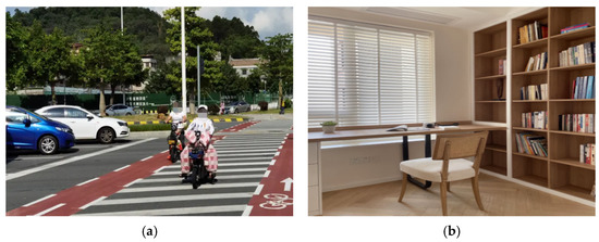
Figure 1.
Spatial relationship examples in different environments. (a) Traffic scene demonstrating spatial relationships between pedestrians, vehicles, and urban infrastructure. (b) Indoor scene showing spatial relationships between furniture and objects.
Spatial front-back relationships describe the relative depth ordering between objects, indicating which objects are positioned nearer or farther in the perceived spatial arrangement. Unlike other spatial relationships that may be scenario-specific (such as inside-outside relationships being more relevant in architectural contexts), front-back relationships are universally present whenever multiple objects coexist within a scene, making them fundamental to comprehensive scene understanding. Figure 2 exemplifies this concept in a typical road scene, where vehicle A (middle, foreground) is positioned closest to the camera, while vehicles B (right, background) and C (left, background) appear at greater depths. This configuration creates distinct front-back relationships: vehicle A is clearly positioned in front of both vehicles B and C. Meanwhile, vehicles B and C demonstrate a more subtle front-back relationship, occupying similar depth planes with only minor depth variations. This comprehensive example illustrates that front-back relationships exist across a spectrum of depth differences—from pronounced disparities (A in front of B/C) to nuanced variations (B versus C).
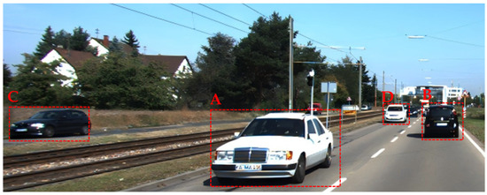
Figure 2.
Spatial front-back relationships in a road scene.
2.2. Formal Definition and Mathematical Framework
Although spatial front-back relationships are intuitively understood, the field lacks a consistent formal definition for computationally determining these spatial relationships between objects in images. The primary obstacle lies in the inherent constraints of two-dimensional (2D) image representation, where pixel coordinates cannot directly encode the three-dimensional (3D) spatial relationships between objects. To establish a formal definition that reflects true spatial front-back positioning, it is necessary to work within a coordinate system that preserves depth information. Therefore, we transform the representation from pixel coordinates to a camera coordinate system. As shown in Figure 3, to determine the spatial front-back relationship between objects, we need to map them to the camera coordinate system to accurately determine this relationship. In this transformation, we define the object that is closer to the camera origin along the depth axis as the “front” object (object A), while the object that is farther from the camera origin along the depth axis is designated as the “back” object (object B, C, or D). These objects together form front-back relationship pairs. This definition aligns with human intuition about depth perception, where objects closer to the camera viewpoint appear in front of those that are more distant. By quantifying spatial relationships in terms of relative distance within a 3D coordinate space rather than 2D image positions, we can more accurately model the true physical arrangement of objects in the scene, despite the dimensional compression that occurs during image capture. We also consider cases where two objects have the same depth relative to the camera coordinate system center, making it impossible to distinguish a front-back relationship between them. We designate this condition as “same depth”, as exemplified by objects B and C in Figure 3.
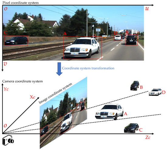
Figure 3.
Transformation from pixel coordinates to camera coordinate system for defining spatial front-back relationships.
Within this camera coordinate system framework, we formalize these spatial front-back relationships by introducing a comparison function R(S, O). We define three types of spatial front-back relationships: F&B (the subject is in front of the object), B&F (the subject is behind the object), and S&D (the subject and object have the same depth with no distinguishable front-back ordering), and established their symbolic representation as follows,
where R(S, O) = −1 indicates that in the camera coordinate system, the subject has a depth less than the object, R(S, O) = +1 signifies that the subject’s depth exceeds that of the object, R(S, O) = 0 denotes that both the subject and object are situated at equivalent depths. Here, “subject” and “object” follow the conventions of human language, where the “subject” is mentioned first and the “object” is mentioned subsequently, both “subject” and “object” are referring to objects. With this framework, the spatial front-back relationship between any pair of objects can be directly represented as a triplet <subject-conf, object-conf, spatial front-back relationship type-conf>, where each element includes its respective confidence score [14,29]. The spatial front-back relationships O between objects across the entire image can be constructed as a set of these triplets,
where Sub Ai, i = 1, 2, …, n, and Obj Bj, j = 1, 2, …, m, are the subjects and the corresponding objects in the image, conf means the corresponding confidence level.
3. Spatial Front-Back Relationship Recognition Framework Design
To accurately identify spatial front-back relationships between objects in images and output results in the form of triplets, we introduce a novel spatial front-back relationship recognition framework called SFBR-PSortNet. The core motivation of our network stems from the observation that bottom keypoints of objects naturally encode relative depth information in the scene. Based on this insight, we design a Partition Sorting mechanism that transforms spatial relationship recognition into a learnable ordering problem, enabling effective spatial reasoning without explicit 3D supervision.
As illustrated in Figure 4, SFBR-PSortNet employs a fully convolutional encoder–decoder architecture that processes visual information through sequential downsampling via convolution operations and upsampling via transposed convolution operations to capture features at multiple scales. The multi-scale feature extraction is crucial for handling objects of varying sizes and ensuring robust spatial relationship detection across different scales. The network then generates multiple prediction heads through convolution layers, predicting category attributes, object width and height in the image, offsets, and front-back ordering values of object bottom keypoints [30,31]. Each prediction head is specifically designed to capture different aspects of spatial relationships: geometric properties for precise localization and front-back ordering values for depth reasoning.

Figure 4.
Architecture overview of SFBR-PSortNet.
Our key technical contribution is the Partition Sorting mechanism, which formulates spatial front-back relationship recognition as an ordering prediction problem by predicting front-back ordering values for each bottom keypoint, effectively determining the front-back relationships between objects. This design enables the network to learn spatial orderings directly from data while maintaining computational efficiency. This mechanism is seamlessly integrated into the neural network through specialized loss functions that guide the learning process. The loss functions are designed to enforce consistent ordering constraints while preserving end-to-end differentiability. By combining bottom keypoint detection with spatial reasoning, SFBR-PSortNet constructs a comprehensive relationship graph and outputs results as triplets, thereby completing the spatial front-back relationship recognition. The complete system architecture diagram and pipeline integration details are provided in Appendix A.
3.1. Bottom Keypoint Detection
Bottom keypoints refer to the points where objects contact the ground or the lowest feature points of objects in an image, which provide unique advantages in spatial front-back relationship reasoning. Unlike traditional center [31,32] points or bounding boxes [9], bottom keypoints naturally encode depth information of objects in three-dimensional space. For objects resting on a common ground plane, perspective projection creates a specific geometric relationship: objects closer to the observer have their bottom keypoints positioned lower in the image frame, while objects farther from the observer have their bottom keypoints positioned higher in the image. This ground-plane perspective principle provides a critical cue for inferring spatial front-back relationships between objects from a single two-dimensional image, without relying on complex depth sensors or multi-view information.
To validate this hypothesis empirically, we analyzed the correlation between bottom keypoint positions and depth values using the KITTI dataset [28]. We observed the relationship between the distance from bottom keypoints to the image bottom and their corresponding ground truth depth values. To quantify this relationship, we initially model a general n-th-order polynomial relationship:
where D(x) represents the depth value, x denotes the distance from the object’s bottom keypoint to the image bottom (in pixels), and ai are the coefficients to be estimated. To determine the optimal polynomial order for modeling the depth-bottom keypoints relationship, we evaluate candidate models ranging from 1st to 6th order polynomials. The optimal is selected to balance model complexity with fitting accuracy while avoiding potential overfitting issues that may arise with higher-order polynomials. The coefficients ai in are estimated using the Ordinary Least Squares (OLS) [33] method, which minimizes the sum of squared residuals:
where N = 36,132 represents the total number of observed objects, Dj is the ground truth depth value for the j-th object, xj is the corresponding distance from bottom keypoint to image bottom, and n ∈ {1, 2, 3, 4, 5, 6} represents the polynomial orders evaluated to determine the optimal model complexity. The selection of optimal polynomial order necessitates a rigorous evaluation framework to ensure robust model performance. We adopt the coefficient of determination (R2) as our principal assessment metric, which provides a quantitative measure of the model’s explanatory power in capturing the underlying depth-bottom keypoints relationship:
where Dj represents the ground truth depth, is the predicted depth value from the polynomial model, and is the mean of all ground truth depth values. Based on the comprehensive evaluation using the coefficient of determination, the 4th-order polynomial demonstrates superior fitting performance with an R2 value of 0.8115. Ultimately, we obtained a fourth-order polynomial relationship between the depth of objects in the image and the distance from their bottom keypoints to the image bottom. The complete analysis, including both the scatter plot of data points and the resulting quartic polynomial fit, is presented in Figure 5.
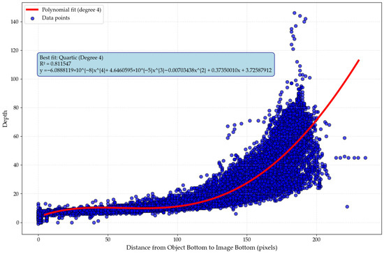
Figure 5.
Scatter plot of bottom keypoint distance to image bottom versus ground truth depth values with fitted quadratic curve.
This strong correlation coefficient demonstrates a robust statistical relationship, validating our hypothesis that objects with bottom keypoints closer to the image bottom are physically closer to the observer, while those with bottom keypoints positioned higher in the image frame are located farther away. Naturally, this assumed relationship is established on the foundation that objects operate within a consistent spatial reference plane, such as terrestrial objects on the ground or maritime objects on the water surface. Objects sharing a common reference plane exhibit predictable spatial front-back relationships, which serves as the theoretical foundation for neural network learning.
However, while this statistical validation confirms the theoretical foundation of our approach, the quartic polynomial fitting with only five parameters has inherent limitations for practical applications. Such a simplified mathematical model cannot capture the complex depth semantics required for real-world spatial relationship reasoning, where factors like object occlusions, varying scales, diverse categories, and changing lighting conditions significantly influence depth perception. For robust front-back relationship reasoning in practical scenarios, deep neural networks with millions of parameters are essential, as they possess the representational capacity to learn intricate non-linear mappings and handle complex factors like occlusions, scale variations, and lighting changes. Importantly, this approach maintains robustness even under moderate camera angle variations or surface irregularities, as deep networks can adapt to these geometric variations through training. This empirical evidence of reliable depth cues, combined with the need for enhanced modeling capacity, motivates our adoption of deep convolutional neural networks for bottom keypoint detection.
Our bottom keypoint detection approach follows the Gaussian distribution-based keypoint detection methodology established in human pose estimation approaches like OpenPose [34], as well as object detection networks such as CornerNet [12], CenterNet [31], and ExtremeNet [35]. For an input image I ∈ RW✕H✕3, features are extracted using a backbone network (e.g., ResNet-50 [5]) followed by consecutive convolutional layers, then processed through a decoder to restore spatial dimensions. The abstract features extracted by the encoder are mapped to a prediction head , which is used for predicting the bottom keypoints of objects, where R = 4 is the output stride and C represents the number of bottom keypoint types. Corresponding to the prediction head B, we generate a ground truth heatmap , where a Gaussian circle [12] is placed at the bottom keypoint of each object. This heatmap is formulated as:
where x and y denote pixel coordinates on the , xb and yb are the ground-truth of the bottom keypoint, and is an adaptive parameter determined by the object’s scale and controls the standard deviation of the 2D Gaussian distribution, with w and h being the width and height of the object bounding box. During training, the ground truth bottom keypoints (xb, yb) are obtained from the bottom-center of manually annotated bounding boxes. These coordinates are used to form Gaussian circles on the supervisory heatmap , which serves as the training signal, whereas during inference, the network directly predict the bottom keypoints from the predicted heatmap B. As shown in Figure 6, Figure 6a is the original input image, while Figure 6b,c visualize the Gaussian circles of the bottom keypoints generated on the ground-truth heatmap .

Figure 6.
Two-dimensional Gaussian distribution of the bottom keypoints of the objects. (a) Input image I; (b) ground truth heatmap of the bottom keypoints for the “boat”; (c) ground truth heatmap of the bottom keypoints for the “persons”. These heatmaps are used as supervision targets during training.
For the prediction head B, we apply focal loss to optimize our network [12,31]. For each location (x, y) on the prediction head, we define the loss function as follows:
where α and β are hyper-parameters of the focal loss, α = 2 and β = 4 in our experiments. N is the number of bottom keypoints in image I. x, y, and c denote the x-axis, the y-axis, and the channel in the heatmap of the pixel.
Additionally, we incorporate auxiliary heads: a localization refinement head and a width-height-ordering prediction head . The localization refinement head predicts the offset of each bottom keypoint from its quantized location in the feature map, compensating for the discretization error introduced by strided convolutions. The training loss for the localization refinement head is formulated as:
where N is the number of bottom keypoints, is the predicted offset of the bottom keypoints along the x-axis, is the ground truth offset along the x-axis, is the predicted offset of the bottom keypoints along the y-axis, is the ground truth offset along the y-axis. The first two dimensions of the width-height-ordering prediction head S aims to directly regress the width and height of the object associated with each bottom keypoint, which is crucial for precise object localization especially in cases with occlusion and scale variations. The corresponding loss function for width and height prediction is defined as:
where N is the number of bottom keypoints, w is the predicted width of the object associated with the k-th bottom keypoint, is the ground truth width, h is the predicted height, and is the ground truth height. For both heads, H(z) is the Smooth L1 Loss [8] defined as:
The width and height prediction, combined with bottom keypoint localization, provides necessary support for spatial front-back relationship recognition.
3.2. Partition Sorting
While bottom keypoints provide 2D localization of objects and contain clues about front-back relationships, exploiting these spatial cues to establish a complete ordering among multiple objects requires a systematic approach. As demonstrated in Section 3.1, these front-back clues originate from the ground-plane perspective principle and the statistically validated polynomial relationship between bottom keypoint positions and depth values. Specifically, the vertical distance of a bottom keypoint from the image bottom encodes depth information, where objects closer to the observer have their bottom keypoints positioned lower in the image frame, while objects farther away have their bottom keypoints positioned higher. This relationship, validated with R2 > 0.9 on the KITTI dataset (Figure 5), provides a reliable ordering cue without requiring explicit 3D reconstruction.
Building upon this foundation, we introduce Partition Sorting, which establishes partial ordering based on relative depth positions rather than challenging absolute depth estimations [27,36]. In Partition Sorting, each detected bottom keypoint receives a front-back ordering value serving as a sorting key, with the process beginning by selecting a pivot object and comparing all other objects’ front-back ordering values against it—those with smaller values are pulled in front while those with larger values are pulled behind. When objects have identical or nearly identical ordering values (within a predefined threshold), they remain in their current positions without repositioning, maintaining spatial stability and avoiding unnecessary computational overhead. This process partitions the object set by repeatedly selecting a pivot object and sorting all other objects relative to it, until a complete spatial ordering is established.
Figure 7 illustrates the Partition Sorting algorithm using a real example from the KITTI autonomous driving dataset. In the initial image, four vehicles (A, B, C, D), are detected with their initial front-to-back order as B → C → A → D. The algorithm iteratively selects pivot objects (highlighted in red) and updates their front-back ordering values, progressively establishing the correct spatial ordering: A → C → B → D from front to back. The final sorting result correctly reflects the front-back relationships observed in the original scene, and the algorithm establishes complete spatial front-back relationships among all objects.
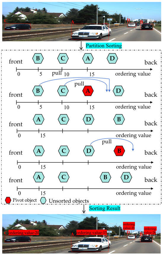
Figure 7.
Schematic diagram of the partition sorting.
Specifically, we extend the architecture of the width-height-ordering head by adding a third channel , to the original width and height channels. This additional channel is dedicated to front-back ordering prediction, where W and H represent the width and height of the input image, respectively, R = 4 denotes the downsampling factor of the network. This detection head is used for predicting the front-back ordering value for each detected object, providing structural support for the Partition Sorting implementation. For each detected bottom keypoint of an object on B, we predict a front-back ordering value at the corresponding position on P. These values serve different purposes depending on the number of objects in the scene. In multi-object scenarios, each front-back ordering value represents a relative numerical value compared to all other objects, reflecting the spatial front-back relationship of this subject relative to other objects. In single-object scenarios, the front-back ordering value serves as a baseline reference for potential multi-object extensions. However, predicting accurate front-back ordering values is non-trivial, as the network must learn to encode complex spatial relationships into numerical rankings. To achieve this, we need to establish a training mechanism that can guide the network to produce ordering values that correctly reflect the actual spatial arrangements in the scene. The iteration mechanism of Partition Sorting can be effectively implemented by constructing a loss function that leverages the backpropagation mechanism of deep convolutional neural networks. As follows:
where N denotes the number of detected bottom keypoints of the objects, and represent the predicted front-back ordering values for the i-th and j-th objects at position (x, y) in P, respectively. R(i, j) indicates the spatial relationship between subject i and object j, where R(i, j) = 0 indicates single-object scenarios (there is no spatial front-back relationship), R(i, j) = F&B indicates subject i is in front of object j, R(i, j) = B&F indicates subject i is behind object j, and R(i, j) = S&D means objects i and j are equivalent depths but are different objects. The loss function uses different formulations for distinct scenarios: logarithmic loss for front-back relationships acts as a smooth ranking loss that encourages correct relative ordering between objects, while squared loss for equivalent depth relationships minimizes prediction differences to ensure consistent values for spatially ambiguous cases. This combination enables meaningful learning of clear spatial relationships while maintaining training stability for ambiguous scenarios.
3.3. Prediction Integration
The SFBR-PSortNet introduces a prediction integration component that fuses information from three detection heads B, S, and L to output spatial front-back relationships between objects in triplet form. The component first determines object detection based on Gaussian distributions predicted by the bottom keypoint detection head B, with peak values indicating detection confidence. Subsequently, width-height-ordering head S directly predicts the width and height of objects at each detected bottom location. Furthermore, an offset head L predicts sub-pixel refinements to compensate for feature map downsampling. Additionally, the additional output dimension P of the S predicts the corresponding front-back ordering value for each object, identifying the spatial front-back relationships R(i, j) between object pairs in the scene,
where Pi represents the front-back ordering values of the subject i, Pj represents the front-back ordering values of the object j, and T = 1.5. The threshold T = 1.5 is designed based on the following considerations: (1) In the driving scenarios studied in this work, front-back ordering differences below 1.5 often fall within the uncertainty range of human depth perception, particularly for objects at similar distances from the camera. (2) Robustness: Given the inherent ambiguity in distinguishing spatial front-back relationships from monocular images, a threshold of 1.5 provides sufficient discriminative power while remaining robust to subtle variations in ordering values.
To quantify the reliability of our spatial front-back relationship predictions, we incorporate a confidence scoring mechanism that reflects the certainty of each predicted front-back relationship. Building upon Equation (12), which determines relationship categories based on Pi and Pj, we calculate a confidence score C(i, j) for each objects pair as:
where T = 1.5 is the same threshold used in Equation (12) for determining S&D spatial front-back relationships, and G = 10 is a normalization factor for spatial front-back relationship categories. This formula assigns higher confidence to object pairs with similar front-back ordering values in the S&D category, while for clear F&B or B&F relationships, larger differences between ordering values receive higher confidence scores. All confidence values are normalized to the range [0, 1] and provide systematic assessment of prediction reliability, enabling more informed interpretation of the spatial relationships, particularly in challenging scenarios with complex object arrangements.
3.4. Architecture Details
The deep convolutional neural network architecture of SFBR-PSortNet is illustrated in Figure 8. The network implements an encoder–decoder framework [37,38,39] with four key components: an encoder for hierarchical feature extraction, a decoder for multi-scale feature reconstruction, parallel prediction heads for spatial relationship prediction, and an integration mechanism for result fusion. This architecture is specifically designed to effectively capture and represent spatial front-back relationships between objects within images, allowing the network to determine which objects are positioned in front of or behind others in the scene.
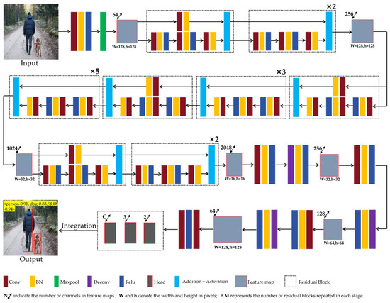
Figure 8.
SFBR-PSortNet architecture Diagram.
The encoder employs ResNet50 [5,40] as the backbone for hierarchical feature extraction. The input image undergoes initial processing through a 7 × 7 convolution and 3 × 3 pooling, producing 64-channel feature maps. Four subsequent residual stages progressively extract multi-scale features: Stage 1 (256 channels), Stage 2 (512 channels), Stage 3 (1024 channels), and Stage 4 (2048 channels). Each residual block utilizes 1 × 1 and 3 × 3 convolutions with skip connections to capture features at different abstraction levels. Stage 1 expands the features to 256 channels, stage 2 increases them to 512 channels, stage 3 further expands to 1024 channels, and stage 4 finally produces 2048-channel feature maps. This hierarchical structure enables the encoder to capture multi-scale visual patterns with varying levels of abstraction, which are essential for accurately predicting spatial front-back relationships between objects in the image.
The decoder module of SFBR-PSortNet adopts a multi-scale feature reconstruction approach to process the encoder’s output. The decoder begins with the high-level feature maps and progressively upsamples them through three consecutive stages. Each stage combines 3 × 3 convolution operations with 4 × 4 deconvolution (transposed convolution) operations to effectively upsample the feature maps while maintaining spatial information [12,31]. The feature dimensions progressively reduce from 256 channels in the initial decoder stage to 128 channels in the second stage, and finally to 64 channels in the third stage. Concurrently, the spatial resolution of the feature maps increases from 32 × 32 in the first stage to 64 × 64 in the second stage, and finally to 128 × 128 in the third stage. This combination of channel dimension reduction and spatial resolution enhancement enables the decoder to gradually recover detailed spatial information while distilling the semantic features captured by the encoder, which is crucial for the subsequent prediction of front-back relationships between objects in the image.
The prediction module processes decoder outputs through three parallel branches, each comprising a 3 × 3 convolution followed by a 1 × 1 convolution for channel adjustment. These heads generate specialized outputs: B for bottom keypoint detection, L for sub-pixel offset refinement, S for object width/height regression and front-back ordering values. These specialized prediction heads capture complementary information about object relationships and feed into the prediction integration component, which aggregates all information to ultimately produce triplet representations of spatial front-back relationships between objects.
4. Experiments and Analysis
4.1. Datasets and Experiment Environment
We evaluated our network on data derived from the KITTI dataset, which comprises a comprehensive collection of 7481 training images and 7518 test images with detailed annotations for multiple object categories (cars, pedestrians, cyclists, trucks, and other traffic participants). Each annotation provides fifteen attributes including: object class, truncation and occlusion levels, observation angle, 2D bounding box coordinates (left, top, right, bottom pixel coordinates), 3D dimensions (height, width, length in meters), 3D spatial position in camera coordinates (x, y, z), and rotation angle around the y-axis. We utilized the z-axis coordinates from the 3D spatial information to determine ground truth front-back relationships between object pairs for our experimental validation. Figure 9 illustrates a representative example from KITTI dataset, showcasing the complex urban driving scenarios that our network aims to address.
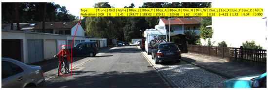
Figure 9.
Representative example from the KITTI dataset.
Since ground truth labels for the official test set are not publicly available and test server submissions are limited, we adopted the standard evaluation protocol used in previous studies. Specifically, we split the original 7481 training samples into three subsets: training (6234 images), testing (623 images), and validation (623 images). We categorize the spatial relationships between object pairs into three classes based on their relative depth positions: F&B, B&F, and S&D. Our training set contains 122,659 object pairs with the following distribution: F&B (84,750 pairs, 69.1%), B&F (24,922 pairs, 20.3%), and S&D (12,987 pairs, 10.6%). This class imbalance reflects the natural distribution of spatial front-back relationships in driving scenarios, and the model is trained on all pairs to learn diverse spatial configurations. For data preprocessing, given the elongated format of KITTI images, which often contain large blank margins without objects, we selectively cropped these empty border regions to focus on areas containing targets, thereby optimizing the input dimensions for regression learning. Additionally, standard data augmentation techniques including image resizing, scaling, and cropping were applied during training to enhance model robustness.
All experiments were performed on a desktop system running Ubuntu 20.04, equipped with an Intel Core i9-10900K CPU (3.7 GHz, 10 cores/20 threads) (Intel, Santa Clara, CA, USA) and dual NVIDIA RTX 3070Ti GPUs (8 GB VRAM each) (NVIDIA, Santa Clara, CA, USA). The software environment included Python 3.8, PyTorch 1.7.0, CUDA 11.1, and cuDNN 8.04. This configuration provided sufficient computational resources for training and evaluating our proposed network.
4.2. Training Configuration
To optimize computational efficiency while maintaining training effectiveness, we implemented a two-stage training strategy. During the initial frozen stage, we preserved the pre-trained ResNet backbone weights while training only the subsequent network layers for 100 epochs with a batch size of 8. This approach significantly reduced memory requirements and computational overhead. In the subsequent fine-tuning stage, we unfroze all network parameters and continued training for an additional 300 epochs. To accommodate the increased memory demands of full network training, we reduced the batch size to 4. Throughout both training stages, we employed the Adam optimizer with an adaptive learning rate scheduling mechanism that dynamically adjusted the learning rate between 5 × 10⁻⁴ and 5 × 10⁻⁶ based on loss progression, ensuring optimal convergence while maintaining computational efficiency. Data augmentation techniques were applied during training to enhance model robustness and generalization capability [41,42]. These included random horizontal flipping (probability = 0.5), random rotation (±10°), and color jittering to increase the diversity of training samples and prevent overfitting.
As illustrated in Figure 10, the training loss curve demonstrates the effectiveness of our two-stage training approach. The curve shows rapid initial convergence during the frozen stage (epochs 0–100), followed by more gradual but steady improvement during the fine-tuning stage (epochs 100–400), ultimately achieving stable convergence with minimal fluctuations.
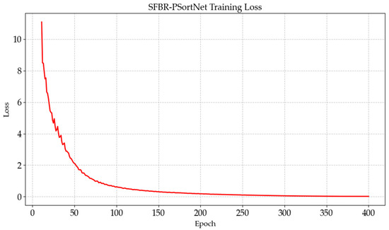
Figure 10.
The training loss curve of the SFBR-PSortNet.
4.3. Metrics and Results
To comprehensively evaluate the performance of our SFBR-PSortNet, we employed multiple standard classification metrics including Accuracy, Precision, Recall, and F1-Score [43,44,45]. These metrics provide multifaceted insights into the model’s capability to correctly determine front-back relationships between object pairs. The performance evaluation was conducted using the following standard metrics:
In these formulas, TP, TN, FP, and FN represent true positives, true negatives, false positives, and false negatives, respectively. For our evaluation, we evaluate spatial front-back relationships for every object pair in the scene, with ground truth relationships determined from actual depth label values. For each relationship category (F&B, B&F, S&D), true positives represent object pairs correctly predicted to have that specific spatial relationship, false positives represent object pairs incorrectly predicted to have that relationship, false negatives represent object pairs that actually have that relationship but were not correctly identified, and true negatives represent object pairs correctly predicted to not have that specific relationship. The metrics are computed based on all pairwise object relationships in the evaluation dataset.
Table 1 presents the detailed performance metrics of our SFBR-PSortNet model on the test set derived from the KITTI dataset across different relationship categories. The model demonstrates strong performance in recognizing both F&B and B&F relationships, achieving high precision and recall values that translate to F1-Score of 0.92 and 0.97, respectively. This indicates that the SFBR-PSortNet model is particularly effective at distinguishing clear front-back relationships between objects. However, the relatively lower performance in the S&D category, with an F1-Score of 0.58, suggests that identifying objects at similar depths presents a more challenging task for the model. This is expected, as subtle depth differences are inherently more difficult to perceive from monocular images. Overall, the SFBR-PSortNet model achieves an impressive Accuracy of 0.93 (93%) across all relationship categories, with overall Precision, Recall, and F1-Score of 0.80, 0.85, and 0.83, respectively. These results validate the effectiveness of our network model in determining spatial front-back relationships between objects.

Table 1.
Performance of SFBR-PSortNet model on the test set.
Additionally, it should be noted that the reported overall accuracy of 0.93 is achieved with the threshold T = 1.5 as specified in Equation (12). To validate this design choice, we conducted comprehensive evaluations on the KITTI validation set using alternative threshold values. As shown in Figure 11 T = 1.5 achieves an accuracy of 0.91 on the validation set, while other thresholds yield lower performance: T = 1.0 (0.89), T = 2.0 (0.87), T = 2.5 (0.88), and T = 3.0 (0.85). These comparative results confirm that T = 1.5 is the optimal threshold choice for spatial front-back relationship recognition.
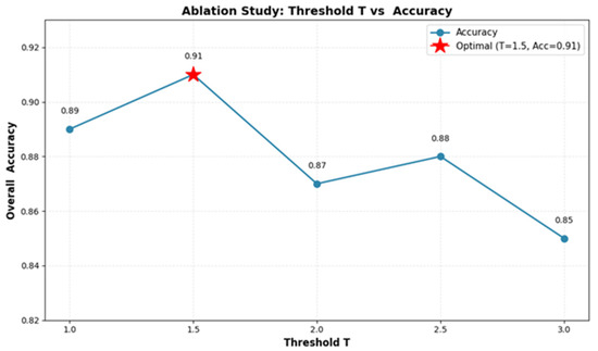
Figure 11.
Statistical analysis of Accuracy vs. threshold T in validation set.
Beyond Accuracy performance, practical deployment requires consideration of computational efficiency. In addition to accuracy metrics, we also evaluate the computational efficiency of our SFBR-PSortNet. Our model contains approximately 33 million parameters and achieves an inference speed of 37.5 ms per image (~27 FPS) on Intel Core i5-11400 @ 2.60 GHz with NVIDIA GeForce RTX 3070 Laptop GPU (8 GB VRAM). The model size is approximately 125 MB, making it suitable for deployment on mainstream gaming laptops, mobile workstations, and edge computing devices with moderate computational resources. These results demonstrate that our approach achieves a good balance between accuracy and computational efficiency.
To visually demonstrate the performance of our SFBR-PSortNet in real-world scenarios, Figure 12 presents several representative qualitative results. A key feature of our visualization approach is the explicit representation of all pairwise spatial relationships in each image using triplets in the form <subject A, object B, SFB> where the relationship is one of F&B, B&F, or S&D. Figure 12a demonstrates SFBR-PSortNet’s capability to accurately identify the front-back relationship between two objects in a simple scenario. More significantly, as shown in Figure 12b, our network model successfully determines and visualizes the complete set of pairwise relationships among all detected objects, even in densely crowded urban traffic scenes with multiple vehicles, proving its robustness in complex multi-object environments. In mixed pedestrian-vehicle scenarios (Figure 12c), the network model correctly recognizes spatial relationships across object categories, with each triplet explicitly annotating the front-back hierarchy.
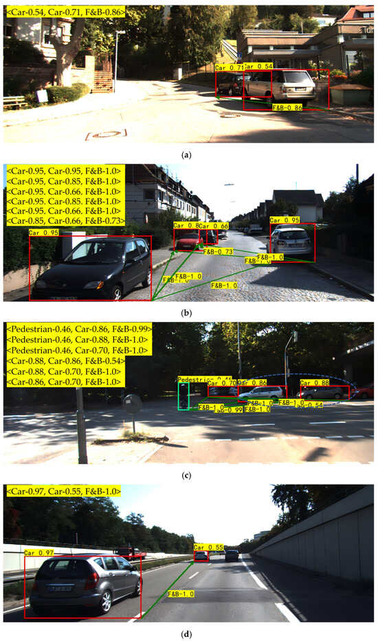
Figure 12.
Several representative qualitative recognition results of SFBR-PSortNet. (a) A simple scenario; (b) Crowded urban traffic scenes; (c) Crowded urban traffic scene with various types of objects included; (d) Scene with darker-colored vehicles and partially occluded objects. Green arrows connect two objects, with the spatial relationship type displayed at the midpoint of the arrow.
While our network model demonstrates strong performance across various scenarios, we have identified areas for potential refinement. In certain cases where objects present near-identical depth with minimal spatial separation (indicated by dashed lines in Figure 12c), the model occasionally misclassifies S&D relationships as F&B or B&F categories, which is consistent with the quantitative results in Table 1 and reflects a common challenge in fine-grained spatial reasoning. Additionally, as our network elegantly combines object detection with relationship recognition, we observe that in scenarios involving partial occlusions or objects with darker visual characteristics (Figure 12d), detection sensitivity for some objects may be affected as the model balances its attention between object localization and higher-level relationship reasoning tasks. This observation highlights an interesting aspect of visual cognition hierarchy where processing resources are distributed across multiple levels of scene understanding. Future work will build upon these insights to further enhance the model by refining its spatial discrimination capabilities for objects at similar depths while maintaining the comprehensive triplet-based visualization framework, and by optimizing the balance between detection sensitivity and relationship reasoning to ensure robust performance across diverse real-world scenarios.
4.4. Comparative Analysis
Since dedicated methods specifically addressing spatial front-back relationship recognition remain scarce in the literature, we needed to identify appropriate approaches for meaningful comparison. We first considered several related computer vision tasks that might potentially address spatial relationships. While visual relationship detection [46] methods focus on identifying various types of visual relationships between objects, current approaches primarily object semantic relationships (such as “person riding bicycle” or “cup on table”) rather than spatial geometric relationships like front-back positioning. Similarly, general object detection methods [47] excel at localizing objects but lack inherent spatial relationship reasoning capabilities. Semantic segmentation [48] approaches, though providing detailed pixel-level understanding, do not explicitly model inter-object spatial relationships.
We observed that spatial front-back relationships and depth estimation are inherently interconnected, as the relative depth positioning of objects directly determines their front-back ordering in a scene. In principle, if accurate depth information is available for each object, their spatial relationships can be systematically derived. This fundamental connection makes depth estimation the most theoretically sound and practically viable approach for comparison, providing the necessary foundation for inferring spatial relationships. Based on this rationale, we establish a comparative framework by benchmarking SFBR-PSortNet against state-of-the-art monocular depth estimation algorithms which can indirectly infer spatial front-back relationships through additional processing steps. For this comparison, we selected several top-performing and representative depth estimation methods from recent years that consistently rank among the leading approaches across major benchmark datasets: LapDepth [27], which uses Laplacian pyramid decomposition for effective feature utilization; Monodepth [38], a widely adopted self-supervised model with auto-masking for handling static regions; DFFNet++ [49], which employs multi-scale feature fusion with enhanced attention mechanisms; and AdaBins [50], a transformer-based approach that adaptively bins depth ranges for state-of-the-art performance. These methods represent diverse paradigms including pyramid-based decoding, self-supervised learning, attention-enhanced fusion, and adaptive binning strategies. To ensure fair comparison, all methods utilize pre-trained models trained on the KITTI dataset and are evaluated on identical data splits, eliminating biases from different training conditions and ensuring reliable performance assessment.
However, these depth estimation models present a fundamental challenge: while they provide pixel-wise depth predictions, they lack the capability to identify and localize specific objects in the scene. To bridge this gap and enable meaningful comparison, we designed a comprehensive evaluation pipeline as illustrated in Figure 13. The pipeline processes each input image through two parallel paths: one path utilizes the depth estimation model to generate a pixel-wise depth map, while the other employs an object detection model to identify objects of interest and extract their bounding boxes. For each detected object, we then map its bounding box to the corresponding region in the depth map and compute the average depth value from the central area of the bounding box. This central-area averaging strategy provides a robust depth estimate for each object while minimizing the influence of boundary artifacts and potential detection inaccuracies. The resulting object-level depth values are then ranked to determine spatial front-back relationships, creating a systematic approach that allows depth estimation methods to address the same task as our SFBR-PSortNet. This pipeline ensures that the comparison focuses purely on the core capability of understanding spatial relationships rather than auxiliary tasks like object detection.

Figure 13.
A comprehensive pipeline for spatial front-back relationship recognition integrating depth estimation and object detection models.
Our comparative experiments reveal significant advantages of our proposed SFBR-PSortNet over depth estimation-based approaches. As shown in Table 2, we compare our method against four representative depth estimation methods (Monodepth + Detection, LapDepth + Detection, DIFFNet++ +Detection, and AdaBins + Detection) that are augmented with object detection to enable spatial relationship inference. The results demonstrate that SFBR-PSortNet achieves superior performance with a Precision of 0.80, Recall of 0.85, and F1-Score of 0.83. These results validate the effectiveness of our end-to-end approach specifically designed for spatial front-back relationship recognition, compared to the indirect pipeline combining depth estimation and object detection.

Table 2.
Comparison with depth estimation methods combined with object detection for spatial relationship recognition.
The key technical advantage of our network lies in its unified end-to-end framework that seamlessly integrates object detection and spatial front-back relationship recognition within a single network architecture. Unlike depth estimation methods that require a multi-stage pipeline involving separate object detection, depth map extraction, and post-processing steps, SFBR-PSortNet directly learns to identify objects and their spatial front-back relationships simultaneously. This integzrated design eliminates error propagation between separate modules, enables joint optimization where object detection and relationship recognition mutually reinforce each other during training, and provides computational efficiency by avoiding redundant feature extraction across multiple independent networks. Beyond technical performance, our network offers substantial practical advantages in annotation requirements and training efficiency. Depth estimation methods typically require dense supervision from specialized sensors such as Light Detection and Ranging (LiDAR), Radio Detection and Ranging (radar), or stereo camera systems to generate ground truth depth maps during training. This dependency creates significant barriers including expensive equipment acquisition, complex calibration procedures, and massive pixel-level annotation datasets. In contrast, SFBR-PSortNet operates with lightweight binary annotations of front-back relationships between object pairs, which can be efficiently created by human annotators using standard images without specialized hardware. This fundamental difference dramatically reduces annotation costs and data collection complexity while eliminating dependence on sensor-based ground truth, making our network more accessible and scalable for practical deployment scenarios.
4.5. Robustness Analysis
4.5.1. Visual Condition Variations
In real-world applications, spatial front-back relationship recognition systems must operate reliably under various challenging visual conditions. Two critical factors that significantly impact the performance of computer vision algorithms are image noise and illumination variations. Image noise, commonly introduced by camera sensors, transmission channels, or environmental interference, can degrade feature extraction and keypoint detection accuracy. Similarly, varying lighting conditions—from overcast environments to intense illumination—present substantial challenges for maintaining consistent recognition performance. Therefore, evaluating the robustness of our SFBR-PSortNet under these conditions is essential to validate its practical applicability and deployment readiness in diverse real-world scenarios.
Noise Robustness Evaluation. To evaluate the robustness of our proposed spatial front-back relationship recognition network under noisy conditions, we conducted a comprehensive noise robustness experiment by adding Gaussian white noise with different intensities to the images of the test set. Specifically, we applied Gaussian noise with standard deviations σ of 5, 10, and 15, following the formulation:
where I represents the original input image and N(0, σ2) denotes a Gaussian distribution with zero mean and variance σ2. As illustrated in Figure 14, our SFBR-PSortNet demonstrates remarkable robustness across different noise levels, with relatively modest performance degradation even under strong noise interference. The performance curves clearly show that recall exhibits the most stable performance, decreasing only from 0.85 to 0.82 (a 3.5% drop) as noise intensity increases from σ = 0 to σ = 15, indicating that our network maintains high recognition rates for true front-back relationships even in noisy environments. Precision shows a moderate decline from 0.80 to 0.77 (3.8% reduction), while the F1-Score drops from 0.83 to 0.78 (6.0% decrease), demonstrating the overall stability of the network. Although Accuracy decreases from 0.93 to 0.90, it remains at a high level above 90%, confirming the practical applicability of our network model. It should be noted that as noise intensity increases, there is a gradual increase in miss bottom keypoints detection rates, with some object’s bottom keypoints becoming undetectable under stronger noise interference. This suggests that while the network maintains good spatial front-back relationship classification accuracy for successfully detected object bottom keypoints, the object bottom keypoint detection itself becomes less sensitive in noisy conditions. Despite some challenges in keypoint detection under high noise conditions, our network maintains stable performance for spatial front-back relationship recognition, confirming its practical applicability in real-world scenarios.
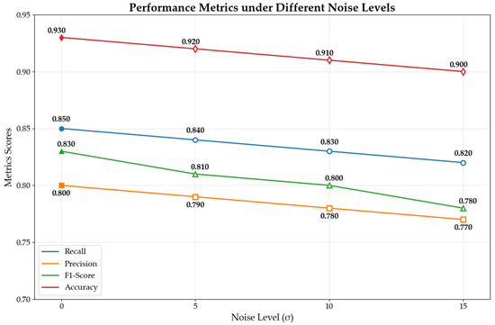
Figure 14.
SFBR-PSortNet performance under different noise conditions.
Illumination Variation Robustness. In addition to noise interference, illumination variation represents another critical challenge for robust spatial front-back relationship recognition. We further examined the performance stability of our network under different lighting scenarios by adjusting the brightness of test images to simulate four illumination conditions: −20% (simulating overcast), 0% (standard), +20% (bright), and +40% (intense lighting). As shown in Figure 15, our network demonstrates good robustness across different brightness conditions, with accuracy maintaining stable performance between 91% and 93% and recall ranging from 83% to 85%. While precision shows some fluctuation, particularly dropping to 73% under +20% lighting conditions, the overall performance remains acceptable. An important point to clarify is that illumination changes, particularly lighting reduction, also affect keypoint detection success rates. When lighting is reduced by 20%, our bottom keypoint detection misses 4.50% of the keypoints, primarily due to reduced visibility of texture features in darker regions. Despite some challenges in keypoint detection under varying illumination conditions, our network maintains stable performance for spatial front-back relationship recognition across different brightness conditions.
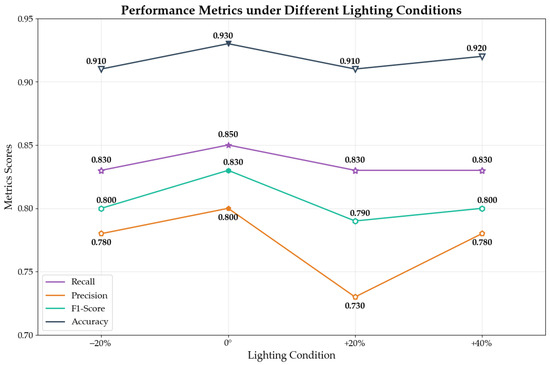
Figure 15.
SFBR-PSortNet performance under different lighting conditions.
4.5.2. Scene Complexity Robustness
Beyond basic visual condition variations, real-world spatial front-back relationship recognition systems must also handle scene complexity challenges. Two particularly demanding scenarios commonly encountered in urban environments are occlusion and multiple overlapping instances. To evaluate the robustness of our SFBR-PSortNet under these challenging conditions, we conduct additional experiments focusing on these two scenarios. For occlusion scenarios, we define the occlusion ratio as the percentage of background object area covered by foreground objects. We compile a specialized test set by collecting images from our dataset that contain occlusion and multiple overlapping instances, where many images are cropped to focus on local regions specifically capturing occlusion scenarios, to conduct qualitative evaluation. Figure 16 shows some representative examples with front-back ordering values and ranking numbers for each detected object. Our qualitative analysis reveals that SFBR-PSortNet demonstrates remarkable robustness when the occlusion ratio remains below 50% (as shown in Figure 16a–c), successfully detecting all target objects and accurately predicting their spatial front-back relationships including cases involving multiple overlapping instances (as shown in Figure 16d–f). However, when the occlusion ratio exceeds 50%, we observe that heavily occluded background objects are missed, which represents a current challenge of our approach, as shown by the white “truck” in Figure 16g and the distant objects in Figure 16h,i. This limitation is partly attributed to insufficient visible features available for heavily occluded objects, suggesting that future work could explore attention mechanisms specifically designed for occluded object detection or incorporate temporal information to improve robustness under severe occlusion conditions.
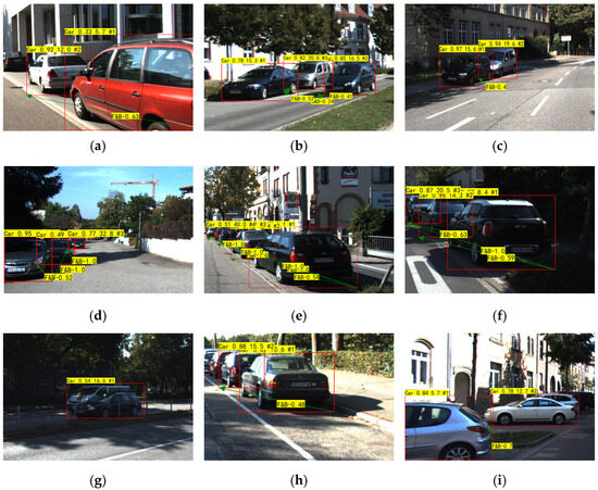
Figure 16.
Spatial front-back relationship recognition results of SFBR-PSortNet under occlusion and multiple overlapping instances. (a) Mild occlusion two-vehicle scenario; (b) Mild occlusion three-vehicle scenario; (c) Mild occlusion two-vehicle scenario; (d) Multiple vehicle overlapping scenario; (e) Complex multi-vehicle overlapping scenario; (f) Dark-colored vehicle overlapping scenario; (g) Heavy occlusion scenario with missed detection; (h) Scene with distant occluded objects; (i) Side-view scene with distant occluded vehicles. Each detected object is labeled with its category, confidence, front-back ordering value, and ranking number (indicated by #). The front-back ordering value represents the relative depth position of each object, where smaller values indicate objects closer to the front. The ranking number (#1, #2, etc.) denotes the sequential order from front to back based on these ordering values. Green arrows connect each pair of objects and indicate the type and confidence of their spatial front-back re.
Furthermore, to demonstrate the effectiveness of our sorting algorithm (Section 3.2) in complex multi-object scenarios, we present a representative case in Figure 17, showing the front-back ordering relationships of 14 objects across different categories (this presentation format is more concise and clear when dealing with numerous objects, compared to displaying detailed spatial relationships for all object pairs). The algorithm successfully processes all objects and establishes correct spatial ordering from the nearest (Pedestrian) to the farthest (Car). This also validates that our SFBR-PSortNet maintains robust performance in high-density scenes with numerous spatial relationships.
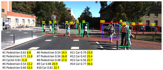
Figure 17.
Front-back ordering results on a multi-object scene. Each object is labeled with #X representing its front-back spatial order (smaller numbers indicate closer objects). To maintain visual clarity with numerous objects, only ordering indices are displayed in the image, while detailed information—object category, confidence score, and front-back ordering value (highlighted in yellow)—is listed below the figure.
Given that our model’s exploration of spatial front-back relationships is predicated on the fundamental assumption that objects reside within a consistent spatial reference plane, it becomes imperative to validate the model’s performance on images exhibiting significant perspective distortions or floor-plane deviations that transcend the assumed reference framework. To comprehensively assess the model’s robustness beyond idealized geometric conditions, we conducted a systematic qualitative evaluation employing strategically designed geometric transformations. Specifically, we performed the following operations on the test set constructed in the occlusion experiment: (1) rotation transformations of 15° and 30° to simulate camera roll movements around the optical axis, representing different degrees of camera tilting that commonly occur in practical deployment scenarios; (2) perspective transformations designed to simulate ground plane tilting effects, including pitch transformations to emulate forward-backward ground plane deviations and yaw transformations to simulate lateral ground plane variations, both creating floor-plane deviations that challenge the planar assumption; and (3) combined affine transformations incorporating rotation, scaling, and shearing to simulate complex camera angle variations under real-world conditions. Figure 18 uses an original image as an example to demonstrate the effects of these transformations.
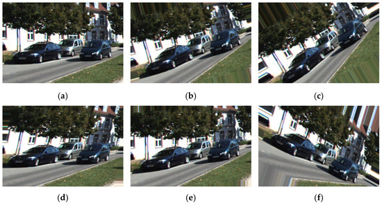
Figure 18.
Geometric transformation results for camera pose and ground plane robustness. (a) Original image I; (b) Image I rotated 15 degrees; (c) Image I rotated 30 degrees; (d) Image I with 15-degree pitch transformation; (e) Image I with 15-degree yaw transformation; (f) Image I with combined geometric transformations.
Figure 19 presents representative experimental results obtained from these transformed images, demonstrating the model’s performance under various geometric distortions. Specifically, Figure 19a–c illustrates the recognition results under 15° rotation transformations, while Figure 19d–f shows the recognition outcomes for 30° rotation transformations, both simulating different degrees of camera roll around the optical axis. Figure 19g–i displays the model’s behavior under 15° pitch transformations that emulate forward-backward ground plane deviations, and Figure 19j–l presents the results for 15° yaw transformations simulating lateral ground plane variations. Finally, Figure 19m–o demonstrates the model’s performance under combined affine transformations incorporating rotation and scaling effects, representing complex real-world camera angle variations. Notably, the model demonstrates promising and encouraging performance on images subjected to pitch and yaw transformations (Figure 19g–l), suggesting that the model maintains decent spatial front-back relationship recognition capabilities when confronted with ground plane deviations. However, the model exhibits significant limitations when dealing with rotation transformations around the optical axis (Figure 19a–f) and combined affine transformations (Figure 19m–o). These results indicate that while the model shows resilience to certain types of geometric distortions and demonstrates promising performance on tilted ground planes, it struggles with camera roll movements, camera angles, and complex combined transformations, highlighting important constraints in its current spatial reasoning framework that warrant further investigation and improvement.
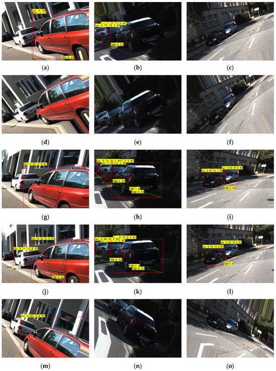
Figure 19.
Spatial front-back relationship recognition results of SFBR-PSortNet under various geometric transformations.
5. Conclusions
In this paper, we introduce SFBR-PSortNet, a novel end-to-end deep convolutional neural network designed for recognizing spatial front-back relationships between objects in images. By leveraging bottom keypoints that naturally encode depth information and incorporating an innovative Partition Sorting mechanism, our network constructs comprehensive spatial relationship graphs between objects. The experimental evaluation based on KITTI demonstrates the effectiveness of our network, achieving an overall accuracy of 93.16% across all relationship categories. Notably, the network model exhibits strong performance in recognizing distinct front-back relationships, with F1-Score of 0.92 and 0.97 for F&B and B&F categories, respectively, thereby validating the efficacy of our proposed network in diverse real-world scenarios.
The SFBR-PSortNet architecture offers an effective strategy by unifying bottom keypoint detection and spatial front-back relationship recognition within a single network framework. This integrated design facilitates effective relationship recognition through the Partition Sorting mechanism while maintaining computational efficiency. The explicit triplet representation (<subject A, object B, spatial front-back relationship>) provides interpretable outputs that are directly applicable to critical domains including autonomous driving, robotics, and augmented reality, where accurate spatial understanding is essential for safe and effective system operation.
While these results are promising, our analysis reveals important areas for improvement. The relatively lower performance in identifying objects at similar depths (S&D category, F1-Score: 0.58) reflects the inherent challenge of discerning subtle depth differences from monocular images. Additionally, SFBR-PSortNet is susceptible to bottom keypoint detection failures under adverse conditions, particularly in the presence of image noise and reduced illumination, which can compromise the accuracy of spatial relationship recognition.
Future research should focus on several key directions. Initially, incorporating temporal information from video sequences to resolve depth ambiguities. Subsequently, developing more robust keypoint detection algorithms for challenging imaging conditions such as poor lighting or partial occlusions. Furthermore, enhancing geometric robustness for non-standard reference plane scenarios including extreme camera angles or irregular terrain. Moreover, exploring selective integration of geometric reasoning, monocular depth estimation, and 3D context methods to enhance spatial understanding while balancing the trade-offs between enhanced capabilities and practical considerations including annotation complexity and computational efficiency.
Author Contributions
Methodology, P.G. and K.Z.; Software, P.G.; Validation, K.Z., T.L., Y.J. and H.Z.; Data curation, P.G.; Writing—original draft, P.G.; Writing—review and editing, K.Z.; Supervision, K.Z., T.L., Y.J. and H.Z.; Funding acquisition, K.Z. All authors have read and agreed to the published version of the manuscript.
Funding
This work was partially supported by the National Natural Science Foundation of China (No. 52071047); partially supported by the National Key Research, and Development Program of China (no. 2021YFB3901501); partially supported by the Distinguished Young Scholar Project of Dalian City (No. 2024RJ012); partially supported by the Fundamental Research Funds for the Central Universities (No. 3132023512); and partially supported by the Dalian City Science and Technology Plan (Key) Project (no. 2024JB11PT007).
Institutional Review Board Statement
Not applicable.
Informed Consent Statement
Not applicable.
Data Availability Statement
Dataset available on request from the authors.
Conflicts of Interest
The authors declare no conflicts of interest.
Appendix A. System Architecture Overview
Figure A1 illustrates the complete system architecture, clarifying how the Partition Sorting integrates into the detection and recognition pipeline. The diagram shows the data flow from input images to final predictions, including the application of the Partition Sorting and related loss function design, demonstrating how our method achieves joint optimization while maintaining compatibility with existing architectures.
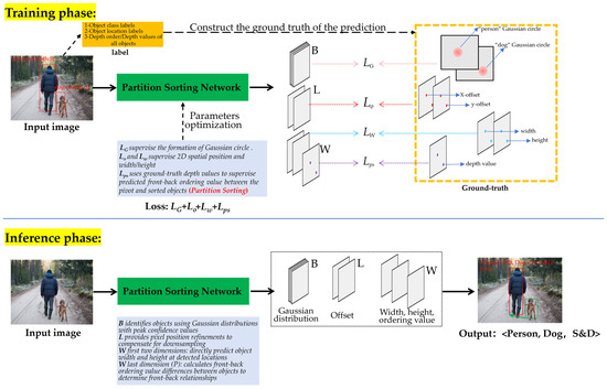
Figure A1.
Overall system architecture of the proposed spatial front-back relationship recognition method during training and inference phases, illustrating the integration of partition sorting with detection and classification components.
References
- Sadeghi, M.A.; Farhadi, A. Recognition Using Visual Phrases; IEEE: Colorado Springs, CO, USA, 2011; pp. 1745–1752. [Google Scholar]
- Krizhevsky, A.; Sutskever, I.; Hinton, G.E. ImageNet classification with deep convolutional neural networks. Commun. ACM 2017, 60, 84–90. [Google Scholar] [CrossRef]
- Simonyan, K.; Zisserman, A. Very deep convolutional networks for large-scale image recognition. arXiv 2014, arXiv:1409.1556. [Google Scholar]
- Szegedy, C.; Liu, W.; Jia, Y.; Sermanet, P.; Reed, S.; Anguelov, D.; Erhan, D.; Vanhoucke, V.; Rabinovich, A. Going deeper with convolutions. In Proceedings of the IEEE Conference on Computer Vision and Pattern Recognition (CVPR), Boston, MA, USA, 7–12 June 2015; pp. 1–9. [Google Scholar]
- Visin, F.; Kastner, K.; Cho, K.; Matteucci, M.; Courville, A.; Bengio, Y. Renet: A recurrent neural network based alternative to convolutional networks. arXiv 2015, arXiv:1505.00393. [Google Scholar] [CrossRef]
- Huang, G.; Liu, Z.; Van Der Maaten, L.; Weinberger, K.Q. Densely connected convolutional networks. In Proceedings of the IEEE Conference on Computer Vision and Pattern Recognition (CVPR), Honolulu, HI, USA, 22–25 July 2017; pp. 2261–2269. [Google Scholar]
- Tan, M.; Le, Q. EfficientNet: Rethinking Model Scaling for Convolutional Neural Networks. In Proceedings of the International Conference on Machine Learning, Long Beach, CA, USA, 9–15 June 2019; pp. 6105–6114. [Google Scholar]
- Ren, S.; He, K.; Girshick, R.; Sun, J. Faster R-CNN: Towards Real-Time Object Detection with Region Proposal Networks. IEEE Trans. Pattern Anal. Mach. Intell. 2017, 39, 1137–1149. [Google Scholar] [CrossRef]
- Redmon, J.; Divvala, S.; Girshick, R.; Farhadi, A. You Only Look Once: Unified, Real-Time Object Detection. In Proceedings of the 2016 IEEE Conference on Computer Vision and Pattern Recognition (CVPR), Las Vegas, NV, USA, 27–30 June 2016; pp. 779–788. [Google Scholar]
- Redmon, J.; Farhadi, A. YOLO9000: Better, Faster, Stronger. In Proceedings of the 2017 IEEE Conference on Computer Vision and Pattern Recognition (CVPR), Honolulu, HI, USA, 21–26 July 2017; pp. 6517–6525. [Google Scholar]
- Farhadi, A.; Redmon, J. YOLOv3: An Incremental Improvement. In Proceedings of the IEEE Conference on Computer Vision and Pattern Recognition (CVPR), Salt Lake City, UT, USA, 18–22 June 2018; pp. 1–6. [Google Scholar]
- Law, H.; Deng, J. CornerNet: Detecting Objects as Paired Keypoints. Int. J. Comput. Vis. 2020, 128, 642–656. [Google Scholar] [CrossRef]
- Tan, M.; Pang, R.; Le, Q.V. Efficientdet: Scalable and efficient object detection. In Proceedings of the IEEE/CVF conference on computer vision and pattern recognition (CVPR), Seattle, WA, USA, 14–19 June 2020; pp. 10781–10790. [Google Scholar]
- Truong, T.; Yanushkevich, S. Visual Relationship Detection for Workplace Safety Applications. IEEE Trans. Artif. Intell. 2024, 5, 956–961. [Google Scholar] [CrossRef]
- Lu, C.; Krishna, R.; Bernstein, M.; Fei-Fei, L. Visual relationship detection with language priors. In Proceedings of the Computer Vision–ECCV 2016: 14th European Conference, Amsterdam, The Netherlands, 11–14 October 2016; pp. 852–869. [Google Scholar]
- Xu, D.; Zhu, Y.; Choy, C.B.; Fei-Fei, L. Scene Graph Generation by Iterative Message Passing. In Proceedings of the IEEE Conference on Computer Vision and Pattern Recognition (CVPR), Honolulu, HI, USA, 21–26 July 2017; pp. 3097–3106. [Google Scholar]
- Dosovitskiy, A.; Beyer, L.; Kolesnikov, A.; Weissenborn, D.; Zhai, X.; Unterthiner, T.; Dehghani, M.; Minderer, M.; Heigold, G.; Gelly, S.; et al. An image is worth 16x16 words: Transformers for image recognition at scale. arXiv 2020, arXiv:2010.11929. [Google Scholar]
- Santoro, A.; Raposo, D.; Barrett, D.G.; Malinowski, M.; Pascanu, R.; Battaglia, P.; Lillicrap, T. A simple neural network module for relational reasoning. In Proceedings of the Conference on Neural Information Processing Systems (NIPS), Long Beach, CA, USA, 4–9 December 2017. [Google Scholar]
- Sharifzadeh, S.; Baharlou, S.M.; Berrendorf, M.; Koner, R.; Tresp, V. Improving Visual Relation Detection using Depth Maps. In Proceedings of the 2020 25th International Conference on Pattern Recognition (ICPR), Milan, Italy, 10–15 January 2021; pp. 3597–3604. [Google Scholar]
- Liu, X.; Gan, M.G.; He, Y. Multi-view visual relationship detection with estimated depth map. Appl. Sci. 2022, 12, 4674. [Google Scholar] [CrossRef]
- Gan, M.G.; He, Y. Adaptive depth-aware visual relationship detection. Knowl.-Based Syst. 2022, 247, 108786. [Google Scholar] [CrossRef]
- Yang, J.; Lu, J.; Lee, S.; Batra, D.; Parikh, D. Graph r-cnn for scene graph generation. In Proceedings of the European conference on computer vision (ECCV), Munich, Germany, 8–14 September 2018; pp. 670–685. [Google Scholar]
- Hudson, D.A.; Manning, C.D. Compositional attention networks for machine reasoning. arXiv 2018, arXiv:1803.03067. [Google Scholar] [CrossRef]
- Chen, B.; Xu, Z.; Kirmani, S.; Ichter, B.; Sadigh, D.; Guibas, L.; Xia, F. SpatialVLM: Endowing Vision-Language Models with Spatial Reasoning Capabilities. In Proceedings of the 2024 IEEE/CVF Conference on Computer Vision and Pattern Recognition (CVPR), Seattle, WA, USA, 16–22 June 2024; pp. 14455–14465. [Google Scholar]
- Wang, H.; Liu, X.; Li, Y.; Xing, G. Depth Estimation Method for Monocular Images Combined with Position Estimation. In Proceedings of the 2024 13th International Conference of Information and Communication Technology (ICTech), Xiamen, China, 12–14 April 2024; pp. 295–299. [Google Scholar]
- Feng, Z.; Yang, L.; Jing, L.; Wang, H.; Tian, Y.; Li, B. Disentangling object motion and occlusion for unsupervised multi-frame monocular depth. In European Conference on Computer Vision; Springer Nature: Cham, Switzerland, 2022; pp. 228–244. [Google Scholar]
- Song, M.; Lim, S.; Kim, W. Monocular Depth Estimation Using Laplacian Pyramid-Based Depth Residuals. IEEE Trans. Circuits Syst. Video Technol. 2021, 31, 4381–4393. [Google Scholar] [CrossRef]
- Liu, Z.; Wu, Z.; Tóth, R. SMOKE: Single-Stage Monocular 3D Object Detection via Keypoint Estimation. In Proceedings of the 2020 IEEE/CVF Conference on Computer Vision and Pattern Recognition Workshops (CVPRW), Seattle, WA, USA, 14–19 June 2020; pp. 4289–4298. [Google Scholar]
- Ding, M.; Liu, Y.; Shi, Y.; Lan, X.; Zheng, N. Dual Graph Attention Networks for Multi-View Visual Manipulation Relationship Detection and Robotic Grasping. IEEE Trans. Autom. Sci. Eng. 2025, 22, 13694–13705. [Google Scholar] [CrossRef]
- Lu, Q.; Jing, Y.; Zhao, X. Bolt Loosening Detection Using Key-Point Detection Enhanced by Synthetic Datasets. Appl. Sci. 2023, 13, 2020. [Google Scholar] [CrossRef]
- Zhou, X.; Wang, D.; Krähenbühl, P. Objects as Points. arXiv 2019, arXiv:1904.07850. [Google Scholar]
- Feng, Y.; Lei, Y.; Yang, X.; Xu, J.; Liu, X.; Xiao, B.; Xu, Y. SIMMKD: Simple Mask-Flow Keypoint Detection for Both Typhoon Detection and Typhoon Eye Location. In Proceedings of the ICASSP 2024—2024 IEEE International Conference on Acoustics, Speech and Signal Processing (ICASSP), Seoul, Republic of Korea, 14–19 April 2024; pp. 5605–5609. [Google Scholar]
- Zhang, L.; Yang, T.; Jin, R. Online Stochastic Linear Optimization: One-Shot SGD and Beyond. J. Mach. Learn. Res. 2021, 22, 1–38. [Google Scholar]
- Cao, Z.; Hidalgo, G.; Simon, T.; Wei, S.-E.; Sheikh, Y. OpenPose: Realtime Multi-Person 2D Pose Estimation Using Part Affinity Fields. IEEE Trans. Pattern Anal. Mach. Intell. 2021, 43, 172–186. [Google Scholar] [CrossRef]
- Zhou, X.; Zhuo, J.; Krähenbühl, P. Bottom-Up Object Detection by Grouping Extreme and Center Points. In Proceedings of the 2019 IEEE/CVF Conference on Computer Vision and Pattern Recognition (CVPR), Long Beach, CA, USA, 15–20 June 2019; pp. 850–859. [Google Scholar]
- Godard, C.; Aodha, O.M.; Firman, M.; Brostow, G. Digging into Self-Supervised Monocular Depth Estimation. In Proceedings of the 2019 IEEE/CVF International Conference on Computer Vision (ICCV), Seoul, Republic of Korea, 27 October–2 November 2019; pp. 3827–3837. [Google Scholar]
- Ronneberger, O.; Fischer, P.; Brox, T. U-Net: Convolutional Networks for Biomedical Image Segmentation. In Medical Image Computing and Computer-Assisted Intervention–MICCAI 2015; Springer: Cham, Switzerland, 2015; pp. 234–241. [Google Scholar]
- Luo, H.; Li, J.; Cai, L.; Wu, M. STrans-YOLOX: Fusing Swin Transformer and YOLOX for Automatic Pavement Crack Detection. Appl. Sci. 2023, 13, 1999. [Google Scholar] [CrossRef]
- ur Rehman, A.; Belhaouari, S.B.; Kabir, M.A.; Khan, A. On the Use of Deep Learning for Video Classification. Appl. Sci. 2023, 13, 2007. [Google Scholar] [CrossRef]
- Cheng, B.; Misra, I.; Schwing, A.G.; Kirillov, A.; Girdhar, R. Masked-attention Mask Transformer for Universal Image Segmentation. In Proceedings of the IEEE/CVF Conference on Computer Vision and Pattern Recognition (CVPR), New Orleans, LA, USA, 19–24 June 2022; pp. 1290–1299. [Google Scholar]
- Na, Y.-H.; Kim, D.-K. Deep Learning Strategy for UAV-Based Multi-Class Damage Detection on Railway Bridges Using U-Net with Different Loss Functions. Appl. Sci. 2025, 15, 8719. [Google Scholar] [CrossRef]
- Hwang, D.; Kim, J.-J.; Moon, S.; Wang, S. Image Augmentation Approaches for Building Dimension Estimation in Street View Images Using Object Detection and Instance Segmentation Based on Deep Learning. Appl. Sci. 2025, 15, 2525. [Google Scholar] [CrossRef]
- Munir, M.A.; Khan, M.H.; Khan, S.; Khan, F. Bridging Precision and Confidence: A Train-Time Loss for Calibrating Object Detection. In Proceedings of the IEEE/CVF Conference Computer Vision and Pattern Recognition (CVPR), Vancouver, BC, Canada, 17–24 June 2023. [Google Scholar]
- Xu, R.; Chen, C.; Peng, J.; Li, C.; Huang, Y.; Song, F.; Yan, Y.; Xiong, Z. Toward RAW Object Detection: A New Benchmark and a New Model. In Proceedings of the IEEE/CVF Conference Computer Vision and Pattern Recognition (CVPR), Vancouver, BC, Canada, 17–24 June 2023; pp. 13384–13393. [Google Scholar]
- Alotaibi, A.; Alatawi, H.; Binnouh, A.; Duwayriat, L.; Alhmiedat, T.; Alia, O.M. Deep Learning-Based Vision Systems for Robot Semantic Navigation: An Experimental Study. Technologies 2024, 12, 157. [Google Scholar] [CrossRef]
- Kim, J.; Park, J.; Park, J.; Kim, J.; Kim, S.; Kim, H.J. Groupwise query specialization and quality-aware multi-assignment for transformer-based visual relationship detection. In Proceedings of the IEEE/CVF Conference on Computer Vision and Pattern Recognition (CVPR), Seattle, WA, USA, 17–18 June 2024; pp. 28160–28169. [Google Scholar]
- Cheng, T.; Song, L.; Ge, Y.; Liu, W.; Wang, X.; Shan, Y. Yolo-world: Real-time open-vocabulary object detection. In Proceedings of the IEEE/CVF Conference on Computer Vision and Pattern Recognition (CVPR), Seattle, WA, USA, 17–18 June 2024; pp. 16901–16911. [Google Scholar]
- Kweon, H.; Yoon, K.J. From sam to cams: Exploring segment anything model for weakly supervised semantic segmentation. In Proceedings of the IEEE/CVF Conference on Computer Vision and Pattern Recognition (CVPR), Seattle, WA, USA, 17–18 June 2024; pp. 19499–19509. [Google Scholar]
- Zhou, H.; Greenwood, D.; Taylor, S. Self-Supervised Monocular Depth Estimation with Internal Feature Fusion. arXiv 2021, arXiv:2110.09482. [Google Scholar] [CrossRef]
- Bhat, S.F.; Alhashim, I.; Wonka, P. AdaBins: Depth Estimation Using Adaptive Bins. In Proceedings of the IEEE/CVF Conference on Computer Vision and Pattern Recognition (CVPR), Nashville, TN, USA, 20–25 June 2021; pp. 4009–4018. [Google Scholar]
Disclaimer/Publisher’s Note: The statements, opinions and data contained in all publications are solely those of the individual author(s) and contributor(s) and not of MDPI and/or the editor(s). MDPI and/or the editor(s) disclaim responsibility for any injury to people or property resulting from any ideas, methods, instructions or products referred to in the content. |
© 2025 by the authors. Licensee MDPI, Basel, Switzerland. This article is an open access article distributed under the terms and conditions of the Creative Commons Attribution (CC BY) license (https://creativecommons.org/licenses/by/4.0/).