Article

Research on Landslide Displacement Prediction Using Stacking-Based Machine Learning Fusion Model

1
China Academy of Railway Sciences Group Co., Ltd., Chengdu 610032, China
2
Northwest Research Institute Co., Ltd. of C.R.E.C., Lanzhou 730070, China
3
Institute of Geotechnical and Underground Engineering, Shandong University, Jinan 250061, China
*
Author to whom correspondence should be addressed.
Appl. Sci. 2025, 15(21), 11747; https://doi.org/10.3390/app152111747
Submission received: 23 September 2025 / Revised: 28 October 2025 / Accepted: 30 October 2025 / Published: 4 November 2025

Abstract

To address the issues of the insufficient accuracy and weak generalization capabilities of single models in landslide displacement prediction, this paper proposes a machine learning model fusion prediction method for landslide displacement based on stacking. Taking the landslide displacement data (F) and rainfall (RAINFALL) of the Baishui River landslide in the Three Gorges Reservoir area as the research object, input sequences were constructed through data preprocessing and feature engineering. Prediction models including SVR, XGBoost, Bayesian optimization, and random forest were established. Based on the stacking framework, an integrated landslide displacement prediction model was developed by dynamically weighting the outputs of the base models using prediction accuracy and stability as fusion indicators. The Baishui River landslide, a typical colluvial landslide, was selected as a case study, with typical displacement data from monitoring points ZG118 and XD-01 from December 2006 to December 2012. The results show that the evaluation metrics (R2, ERMSE, and EMAE) for ZG118 and XD-01 demonstrate satisfactory prediction performance. Compared with traditional single models such as a TCN and XGBoost, the proposed integrated model exhibits improved prediction accuracy, providing scientific support for the real-time monitoring and early warning of landslide hazards.

1. Introduction

As a highly destructive and sudden geological disaster, landslides seriously threaten people’s lives and property and the safety of major infrastructure [1]. According to statistics, there will be a total of 3668 geological disasters across the country in 2023, of which landslides account for a quarter [2]. As an area with frequent geological disasters in our country, the Three Gorges Reservoir area is significantly affected by factors such as reservoir water level fluctuations and rainfall, and the dynamic monitoring and accurate prediction of landslide displacement have become key issues in disaster prevention and control [3,4,5]. However, the landslide evolution process is driven by the multi-field coupling mechanism, and the displacement sequence shows complex characteristics such as high nonlinearity and non-stationarity, resulting in obvious deficiencies in the prediction accuracy, generalization ability, and stability of a single model [6,7].
In recent years, machine learning methods such as support vector regression (SVR), extreme gradient lifting (XGBoost), and random forest (RF) have been widely used in landslide displacement prediction and have shown good performance in local feature mining [8,9,10]. Optimization algorithms such as Bayesian optimization are also used for hyperparameter tuning to improve model adaptability. However, due to the limitations of its algorithm mechanism, it is difficult to fully capture the evolution of landslide displacement on multiple time scales, such as the lag in response of SVR to mutations and the sensitivity of XGBoost to outliers. Therefore, integrating multiple complementary models and integrating their advantages has become an important way to improve prediction accuracy and robustness [11,12].
Although there have been studies using static weighting or averaging strategies for model fusion, it still performs poorly in dealing with complex working conditions such as displacement mutations [13]. To this end, this paper proposes a machine learning fusion prediction method for landslide displacement based on stacking architecture, introduces a dynamic weighting mechanism, and takes model accuracy and stability as the fusion index to realize the adaptive weighted integration of base model output. Taking the Baishui River landslide in the Three Gorges Reservoir area as an example, a high-performance displacement prediction model is constructed by integrating SVR, XGBoost, the Bayesian optimization model, a TCN, and random forest, aiming to improve the prediction reliability under complex geological and environmental conditions, and provide a theoretical basis and technical support for the real-time monitoring and intelligent early warning of landslide disasters [14,15].
Specifically, this study seeks to answer the following questions:
(1)
How to construct a dynamic weight fusion mechanism that can adaptively balance the accuracy and stability of the model?
(2)
How much improvement can the fusion model bring in terms of prediction accuracy and stability compared with advanced single models (such as TCN, XGBoost) and traditional models (such as ARIMA)?
(3)
Can the model effectively capture the sudden displacement changes triggered by external factors such as heavy rainfall?

2. Foundation Model

2.1. Support Vector Regression (SVR)

Support vector regression is an extension of the support vector machine (SVM) in regression problems. The goal of SVR is to find an optimal hyperplane so that most of the sample points fall within the spacer band centered on that hyperplane while minimizing the prediction error [16]. By introducing the kernel function, SVR is suitable for high-dimensional and nonlinear landslide displacement sequence modeling, especially for the stationary change segment. However, it lags in response to sudden rainfall and is sensitive to parameter regularization parameter C and interval bandwidth ε, so it needs to be adjusted by an optimization algorithm. SVR achieves this by minimizing the following objective functions, which are widely used in time series prediction data analysis due to their ability to process high-dimensional data and nonlinear relationships [17,18].
Applicability in landslide prediction: SVR can effectively handle the complex nonlinear relationship between displacement and rainfall, historical displacement, and other features through kernel function techniques. Its structural risk minimization principle shows good generalization ability on small samples of landslide monitoring data, and is not easy to overfit. However, it is less efficient for large-scale data computation and is extremely sensitive to the selection of parameters C and γ .
The regression prediction task, the prediction principle of SVR, is as follows:
Objective function:
min w , b , ξ i , ξ i * 1 2 w 2 + C i = 1 n ξ i + ξ i *
where w 2 represents the complexity of the model, C represents the regularization parameters, and ξ i   and   ξ i * represent the relaxation variables, used to handle deviations outside of the ε range.
Constraints:
y i w , ( x i ) b ε + ξ i w , ( x i ) + b y i ε + ξ i * ξ , ξ i * 0
where ε is the ε -threshold for the insensitive loss function, ( x i ) is a high-dimensional mapping of the input feature vector x i , w , ( x i ) indicates the inner product, and SVR uses the ε -insensitive loss function, defined as follows:
L ε y , f x = y f x ε , when y f x > ε 0 ,
The principle of SVR regression prediction is shown in Figure 1 below.

2.2. Extreme Gradient Boosting (XGBoost)

XGBoost is an ensemble tree model based on a gradient boosting framework that improves prediction accuracy by iteratively training decision trees and optimizing objective functions. The core idea is to gradually correct the residuals of the preorder model based on the weighted results of the weak learner [19]. XGBOOST introduces regularization terms (such as L1/L2 regular) to control model complexity, and supports parallel calculation and feature importance evaluation. Hyperparameters such as the learning rate, tree depth, and subsampling rate have significant effects on model performance. XGBoost can automatically identify feature importance and has good robustness for non-stationary and noisy displacement data [20]. However, it is sensitive to outliers and is easy to overfit when the amount of data is small.
Applicability in landslide prediction: XGBoost can automatically learn feature interactions (such as the relationship between the rainfall accumulation effect and displacement change) and provide a feature importance ranking (such as feature importance), which helps to reveal the key drivers affecting landslide displacement. Its regularization and pruning strategies make it insensitive to outliers and can effectively prevent overfitting, making it ideal for processing noisy field monitoring data. However, it should be noted that too many trees may lead to complex models and increase computational overhead.
Objective function:
L t = i = 1 n l y i , y ^ i t + 1 + f t x i + Ω f t
where y ^ i t + 1 is the predicted value of the first t − 1 tree, f t x i is the output of the t tree, and Ω f t is a regular item.
Ω f t = γ T + 1 2 λ w 2
where T is the number of tree nodes, and λ is the L2 regular parameter.
Numerical division guidelines:
G a i n = 1 2 G L 2 H L + λ + G R 2 H R + λ + G L + G R 2 H L + H R + λ λ
where G L / G R is the gradient sum of the left/right subtree samples, and H L / H R is the Hissen sum of the left/right subtree samples.

2.3. Temporal Convolutional Network (TCN)

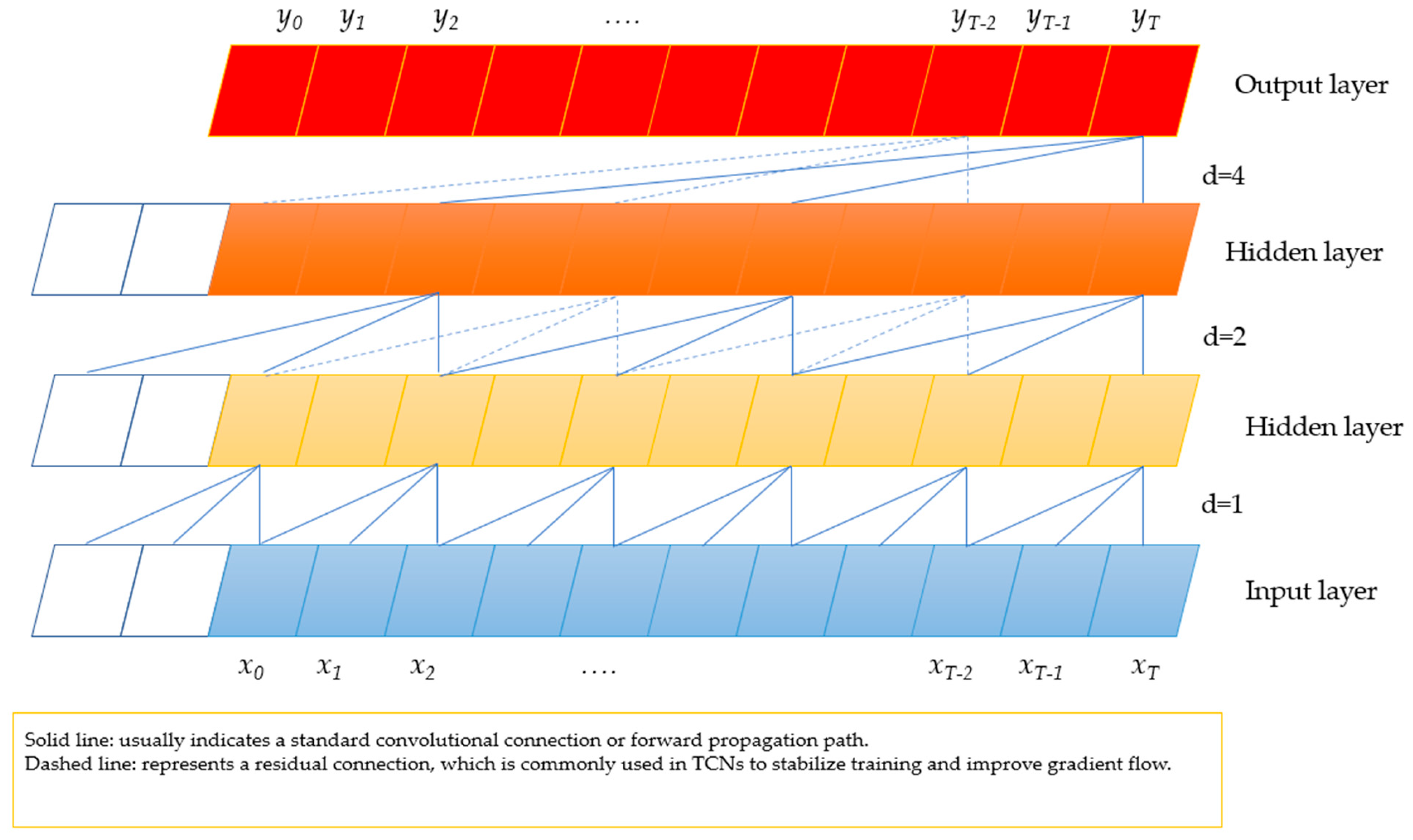
A Temporal Convolutional Network is a deep learning model designed for temporal data that captures long-term dependencies through causal convolution and dilated convolution. The mechanism of a TCN is to ensure that the output relies only on current and historical inputs to avoid future information leakage, and at the same time mitigates the gradient disappearance problem through residual blocks [21]. Its key parameters include convolutional kernel size, expansion factor, and network depth. A TCN shows comparable performance to an RNN/LSTM in sequence modeling tasks and is easier to train in parallel. A TCN can effectively capture the periodic and trend changes in landslide displacement, especially for modeling the displacement response caused by periodic fluctuations in reservoir water level.
A TCN captures long-term dependencies through dilated causal convolution, and its output relies only on current and historical inputs to avoid future information leakage.
In terms of applicability in landslide prediction, the expansion convolutional structure of a TCN enables it to efficiently capture long-term periodic and trend patterns (e.g., the influence of seasonal rainfall and periodic fluctuations in reservoir water level) in the landslide displacement sequence. Its parallelized computational structure (compared to an RNN) makes the training faster and not troubled by gradient disappearance, which is very suitable for long sequence displacement prediction tasks.
Expansion causal convolution: By introducing the expansion factor d, the convolutional kernel covers a wider range of inputs without increasing the number of parameters. For the one-dimensional input sequence xRn and the convolutional kernel f: {0, …, k − 1}→R, the output of the expansion convolution operation F at position s is as follows:
F s = X d f s = i = 0 k 1 f i X s d i
where d is the expansion factor and k is the size of the convolutional nucleus. A TCN alleviates the gradient disappearance problem through residual joining and is suitable for long sequence modeling.
The TCN structure diagram is shown in Figure 2 below.

2.4. Bayesian Optimization

Bayesian optimization is a sequence global optimization algorithm based on Bayesian theorem, which is especially suitable for black box function optimization problems with high computational cost, non-convexity, and unknown derivatives of objective functions. The core mechanism is to balance exploration and utilization by constructing a probabilistic proxy model of the objective function (usually using the Gaussian process) and designing an acquisition function, so as to efficiently find the global optimal solution [22,23].
Key steps in Bayesian optimization include the following:
(1)
Build a priori: Use the Gaussian process as an agent model to model the objective function.
(2)
Choose an acquisition function: Commonly used acquisition functions include expected improvement (EI), upper confidence boundary (UCB), and probability improvement (PI).
(3)
The acquisition function: In each iteration, determine the next evaluation point by optimizing the acquisition function.
(4)
Update proxy model: Update the Gaussian process model with new observations.
Applicability in landslide displacement prediction: Bayesian optimization can efficiently perform global search in the SVR parameter space (e.g., C, γ), and find near-optimal hyperparameter combinations with a small number of iterations, significantly improving the efficiency of model tuning Compared with grid search and random search, Bayesian optimization exhibits better performance with limited computing resources, making it particularly suitable for the hyperparameter tuning of machine learning models.
The goal of Bayesian optimization is to minimize the loss function on the validation set:
x * = arg min x X   f x
where f x is the objective function (e.g., RMSE) that needs to be optimized, X is the parameter space, and x * is the optimal parameter combination.
The Gaussian process is defined as follows:
f x ~ G P m x , k ( x , x )
where m x is a mean function and k ( x , x ) is the covariance function.
The expected improvement (EI) acquisition function is defined as follows:
E I ( x ) = E max 0 , f min f ( x )
where f min is the best function value currently observed.

2.5. Random Forest (RF)

Random forest is a machine learning algorithm based on ensemble learning ideas, and its mechanism improves the generalization ability of the model by constructing multiple decision trees and aggregating the prediction results [24]. The core of the algorithm lies in double randomness: self-service sampling (Bootstrap) is used to generate a differentiated training set for each tree at the data level, and the correlation between trees is reduced through random subspace selection at the feature level. This mechanism effectively balances bias and variance, which can not only explore the spatial diversity of features through a parallel tree structure, but also achieve stable prediction through majority voting or mean strategy. Key parameters such as the number of decision trees, maximum depth, and feature subset size directly affect the model complexity and computational efficiency. Random forests are widely used in classification, regression, anomaly detection, and feature selection due to their overfitting resistance, missing value robustness, and feature importance evaluation capabilities, especially for high-dimensional data and nonlinear relationship modeling scenarios. RF is suitable for displacement prediction under high-dimensional features, and can effectively identify the influence of multiple factors such as rainfall and water level on landslides. Random forests are constructed with multiple decision trees through Bootstrap sampling, and the results are integrated by voting or averaging. Applicability in landslide prediction: RF can effectively handle high-dimensional features (such as multi-period lag displacement, rainfall), is insensitive to missing and outlier values, and has good robustness. The characteristic importance assessment provided by it is helpful to quantify the contribution of environmental factors (such as current rainfall and previous displacement) to the prediction, and provide a reference for the analysis of the landslide mechanism. However, the model interpretability is not as good as that of a single decision tree, and the training time increases linearly with the increase in the number of trees.
Its randomness is reflected in two aspects:
  • Data randomness: Generate a different training subset for each tree through Bootstrap sampling.
  • Feature randomness: When each node is split, k (usually k = m or k = log 2 m ) features are randomly selected from all m features to form a subset of features, and the optimal splitting point is selected from them.
The final prediction result is the average of all decision tree outputs:
y ^ = 1 B b = 1 B T b x
where B is the number of trees, and T b x is the prediction result of the tree b. RF has good overfitting resistance and robustness to missing data.
The RF structure diagram is shown in Figure 3 below:

2.6. Stacking Model

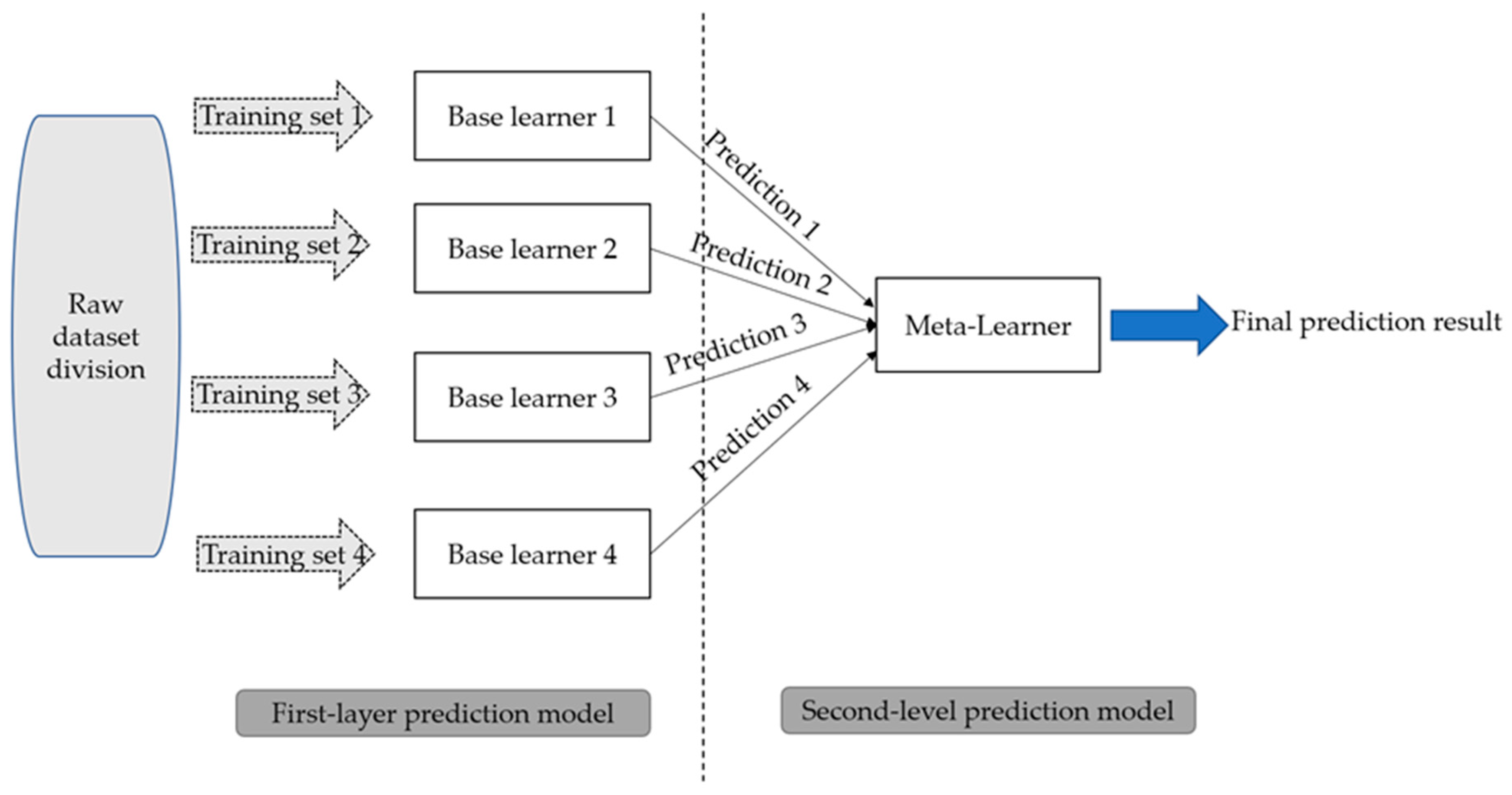
Stacking is an ensemble learning method that improves the generalization ability of a model by combining the prediction results of multiple base learners [25]. The core mechanism is to train a meta-model and use the outputs of different base models as input features for secondary learning, thereby integrating the advantages of each model. The key to stacking lies in the diversity of the base model and the generalization ability of the meta-model, which needs to be cross-verified to avoid data leakage and overfitting. Although the selection of base models and parameter adjustments have a significant impact on the final performance, stacking demonstrates strong accuracy in complex prediction tasks [26].
Applicability in landslide prediction: Stacking can more comprehensively capture the complex mechanism of landslide displacement evolution by integrating the advantages of heterogeneous models such as SVR (nonlinear fitting), XGBoost (feature interaction), TCN (timing dependence), and RF (robustness). Its integrated prediction results are more stable and accurate than any single model, which significantly improves the prediction reliability in sudden events such as heavy rainfall and provides a more powerful tool for landslide early warning. The training process is divided into two layers:
  • Layer 1 (base learner): Use the training data Dtrain to train multiple different base models (e.g., SVR, XGBoost, RF, TCN) independently. Subsequently, these base models are used to predict the validation set Dval, and the prediction results are used as a new feature matrix Zval. At the same time, a prediction Ztest for the test set is also generated.
  • The second layer (meta-learner): The validation set predicts the result Zval and its corresponding real label Yval as a new training set to train the meta-model (usually choose a simple linear model, such as ridge regression, or a model with strong expression ability, such as XGBoost). Finally, the trained meta-model is used to predict feature Ztest for the final prediction of the test set.
The process is shown in Figure 4:

3. Model Fusion Based on Stacking Model

3.1. Dynamic Weighting Mechanism

The stacking fusion mechanism adopts a dynamic weighting strategy, and the weight allocation of the base model comprehensively considers its prediction error (RMSE) and stability (prediction variance), and ensures that the sum of weights is 1 through normalization processing. The formula for defining weights is as follows:
w i = α 1 / R M S E i j = 1 n 1 / R M S E i + 1 α 1 / V a r i j = 1 n 1 / V a r
where R M S E i is the root mean square error of the ith base model in the validation set, and V a r i is the variance of the prediction results of the ith base model in the validation set; α is the accuracy–stability balance factor and n is the total number of base models.
The value range of the precision–stability balance coefficient a is [0, 1], and the search range is small, so the grid search algorithm is used to determine the value of a.

3.2. Stacking Framework Overview

Ensemble learning is a multi-algorithm fusion machine learning method based on statistical learning theory; in general, for a single prediction model, its prediction ac-curacy is a trend of diminishing marginal utility, and stacking ensemble learning is a model integration technology that combines information from multiple prediction models to generate a new model. Different machine learning algorithms are combined in different ways to achieve superior performance over a single algorithm. In the stacking ensemble learning model, it is necessary to analyze the individual prediction ability of each base learner and comprehensively compare the combined effects of each base learner to obtain the best prediction effect of the stacking ensemble learning model.
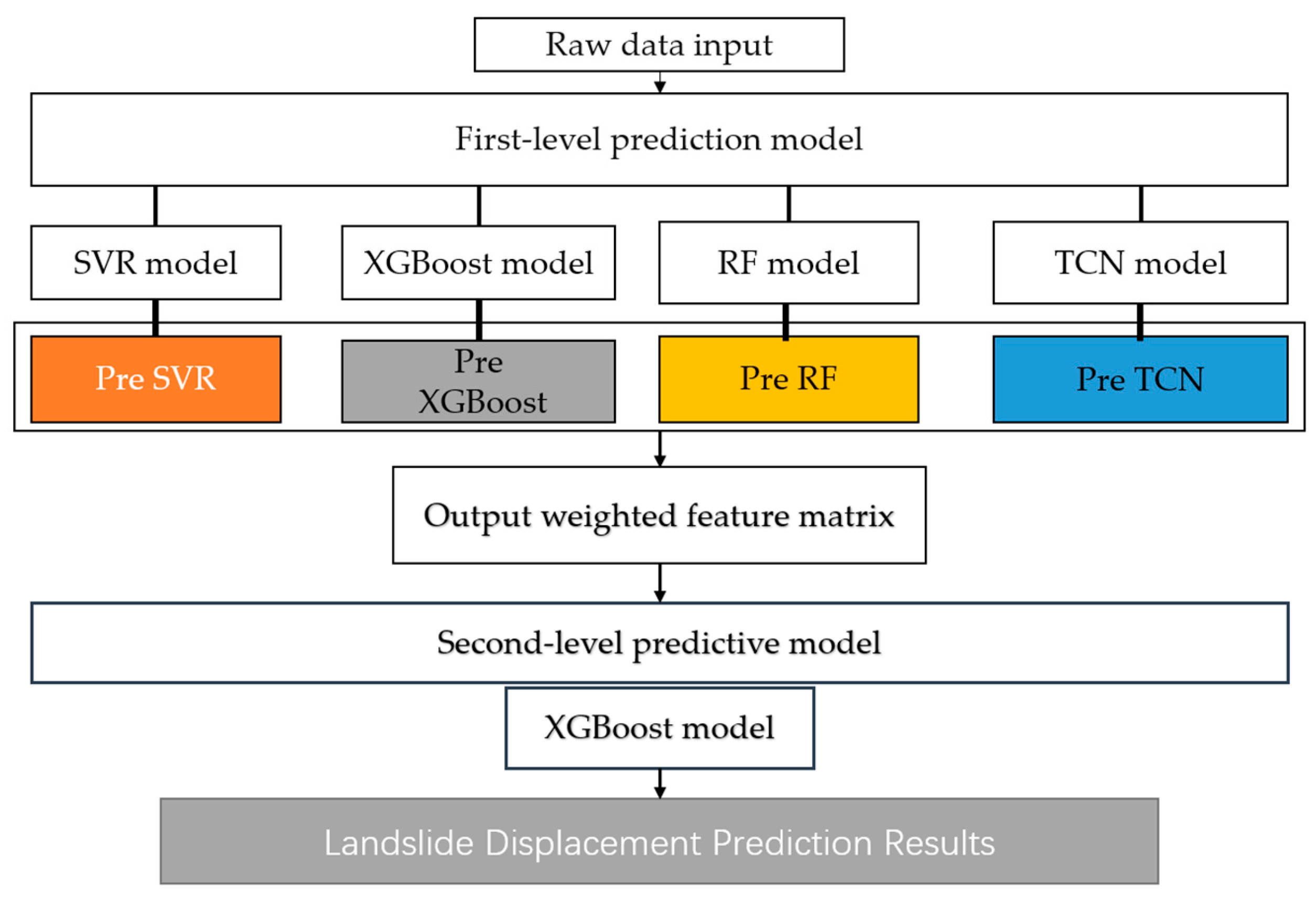
In this paper, the first layer of the stacking model is composed of multiple base learners with complementary principles, including support vector regression (SVR) that is good at nonlinear fitting, extreme gradient lifting (XGBoost) that can automatically identify the importance of features, and is dedicated to capturing long-term time series dependencies as well as random forests (RF) with good robustness. Each base model is trained independently based on the same training set, and the validation set is predicted separately. This process aims to mine diverse potential patterns and features from the displacement sequence. The prediction results of the validation set of the first-layer base model are constructed into a new feature matrix. In this study, a dynamic weight fusion mechanism is introduced as a core innovation, which calculates the adaptive weight of each base model based on the prediction accuracy (RMSE) and stability (variance) of each base model on the validation set, so as to generate new weighted features by the equilibrium coefficient (α). In the second-level prediction model, the XGBoost model is selected as the meta-model, and the meta-model is trained using weighted feature data from the outputs of the first level. The role of the meta-model is not to directly process the raw data, but to learn how to optimally combine the prediction results of each base model, that is, to act as a “decision arbiter” and finally output the integrated displacement prediction value.
The key innovation of this framework is the introduction of a dynamic weighting mechanism, which adaptively adjusts the fusion weights of each base model based on the prediction accuracy and stability indicators on the validation set, instead of using traditional average or static weighting strategies. Ultimately, the meta-learner generates more accurate and stable predictions by integrating the strengths of all base learners.
The stacking-integrated architecture realizes the complementary advantages of heterogeneous models through the collaborative work of the two-layer model, significantly improves the generalization ability and prediction accuracy of the overall model, and is especially suitable for dealing with complex nonlinear regression problems.
Throughout the process, hyperparameters (such as C for SVR, depth for XGBoost, etc.) are adjusted using Bayesian optimization, and the weight coefficient accuracy–stability balance factor α is determined using a grid search algorithm due to the small search range.
The training process of the landslide displacement prediction method based on multi-model dynamic weighted fusion under the stacking framework is as follows:
(1)
Base model selection and hyperparameter optimization: SVR, XGBoost, TCN, and random forest algorithms with large differences and complementary performance are selected as the basic prediction model of the first layer. The hyperparameters of the SVR model are optimized by Bayesian optimization, and the hyperparameters of other models are set according to pre-experiments and empirical settings.
(2)
Independent training of base models: Using the divided training set data, each foundation model is trained independently to ensure that each model can fully learn the features of the displacement sequence.
(3)
Dynamic weight calculation and meta-feature construction: The trained foundation models are applied to the validation set to obtain their respective prediction results. Based on the prediction accuracy (RMSE) and stability (variance) of each model on the validation set, the corresponding fusion weight is calculated by using the dynamic weight formula. The predictions of each foundation model are multiplied by their dynamic weights to obtain weighted predicted values, and these weighted predictions are combined into a new meta-feature dataset.
(4)
Meta-model training and fusion prediction: The XGBoost meta-model of the second layer is trained by taking the newly generated meta-feature dataset as the input and the real displacement value of the corresponding validation set as the target. The meta-model learns how to optimally integrate the weighted predictions of each basic model to form the final stacking fusion prediction model.
The specific process is shown in Figure 5 below.

4. Prediction of Landslide Displacement in Baishui River

4.1. Overview of Engineering Geology

The Baishui River landslide is located on the south bank of the Yangtze River, 56 km away from the dam site of the Three Gorges Dam, and belongs to Baishui River Village, Shazhenxi Town. The geographical coordinates are longitude 110°32′09″ and latitude 31°01′34″. It is located in a single-oblique slope terrain, distributed in a stepped manner, and the sliding body is mainly composed of Quaternary residual slope accumulation soil and landslide accumulation soil, including silty clay and gravel soil. The landslide body is located in the wide valley of the Yangtze River, with a single slope and a low slope in the south, spreading out to the Yangtze River in a stepped manner. Its trailing edge elevation is 410 m, bounded by the geotechnical boundary, the front edge reaches the Yangtze River, and the east and west sides are bounded by bedrock ridges, with an overall slope of about 30°. Its north–south length is 600 m, east–west width is 700 m, the average thickness of the sliding body is about 30 m, and the volume is 1260 × 104 m3.
The seven GPS monitoring points laid out in the initial monitoring stage are distributed on three longitudinal profiles, and there are three GPS monitoring points in the middle section, and two GPS monitoring points are arranged on both sides. Subsequently, four GPS monitoring points were added in the landslide warning area, and one GPS reference point was established on the bedrock ridges on the east and west sides of the periphery of the sliding body.
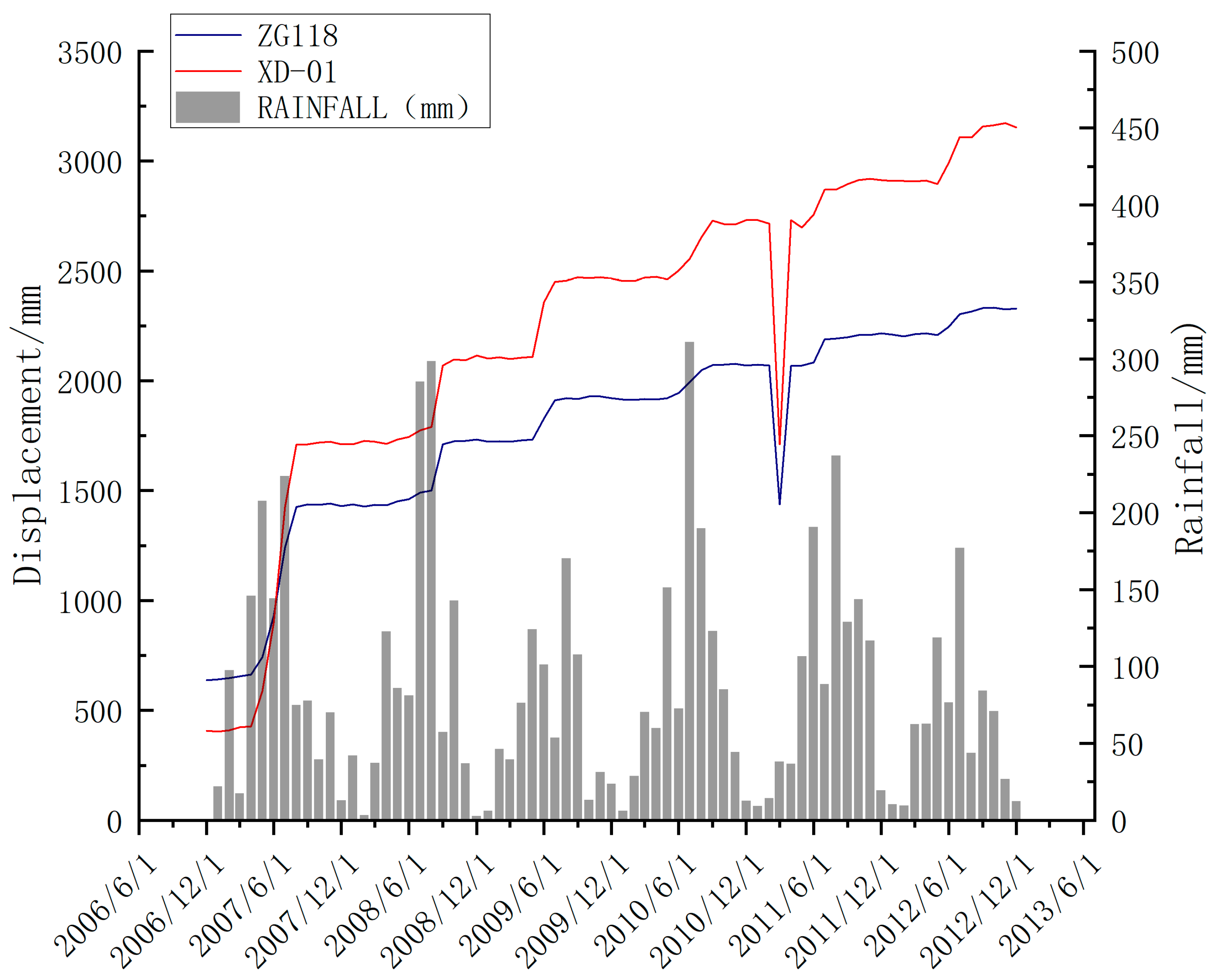
The data come from the National Glacier and Frozen Soil Desert Science Data Center (https://s.ncdc.ac.cn/portal/ accessed on 30 October 2024). The dataset used in this study was selected from GPS monitoring points ZG118 and XD-01, with a time span from December 2006 to December 2012, totaling 72 monthly data points. The dataset mainly includes the following variables:
Time: Observation year and month.
F_ZG118 (mm): Cumulative displacement value at monitoring point ZG118.
F_XD01 (mm): Cumulative displacement value at monitoring point XD-01.
RAINFALL (mm): Monthly rainfall data.
The GPS monitoring data curves of the landslide displacement at monitoring points ZG118 and XD-01 are shown in Figure 6 and Figure 7:

4.2. Data Preprocessing

Based on the 72 GPS observation data of the ZG118 and XD-1 monitoring points obtained from December 2006 to December 2012, there are some data anomalies in the original data obtained, which seriously affect the prediction accuracy of the model; therefore, the following data preprocessing methods are adopted: original data → exception correction → missing imputation → effect verification.

4.2.1. The Grubbs Criterion Detects Outliers

To monitor outliers at the beginning of the Grubbs criteria, the formula is as follows:
G = X i μ σ
where X i is the data point to be detected, and μ , σ are the mean and standard deviation of the data series.
Specific steps:
The mean values of the ZG118 sequence (excluding March 2011) were calculated as μ = 2073.4 mm and standard deviation σ = 18.7 mm. Detected March 2011 value X i = 1437.8   mm .
G = 1437.8 2073.4 18.7 = 33.9
The Grubbs threshold table showed that the significance level was α = 0.05, and the number of samples n = 60 was a = 3.15 and b > c, which was G c r i t = 3.15 , G > G c r i t judged to be an outlier. At the same time, in March 2011, no extreme rainfall or water level changes capable of causing such a large displacement were recorded, and the abrupt change point did not match the trends before or after, so it was concluded to be a monitoring error.

4.2.2. Three-Dimensional Spline Interpolation Correction

The cubic spline function S(t) is constructed by using adjacent time series points, and the interpolation is solved.
Formula:
X r = S t w
The final partial substitution results for outliers are shown in Table 1.
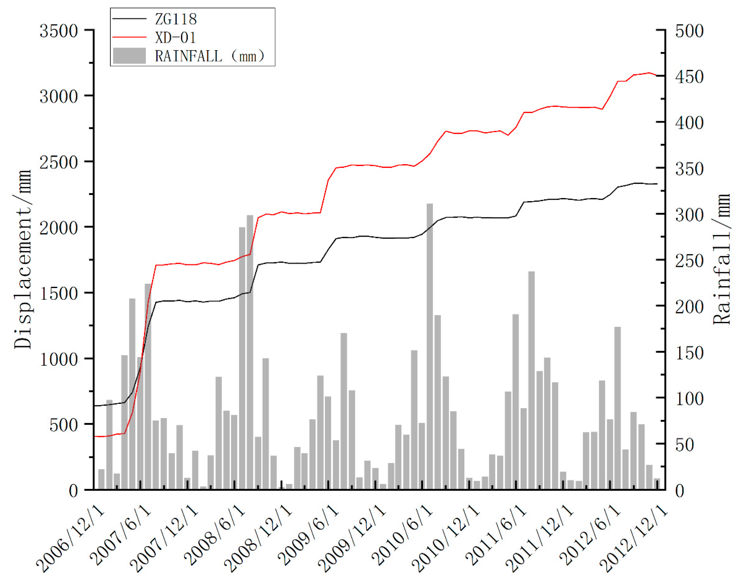
The cumulative landslide displacement and rainfall monitoring curves of the ZG118 and XD-1 monitoring points from December 2006 to December 2012 after data preprocessing are shown in Figure 8.

5. Landslide Displacement Prediction

5.1. Experimental Design and Model Training

5.1.1. Data Division and Feature Engineering

Based on the displacement data of 72 periods from December 2006 to December 2012 at the ZG118 and XD-01 monitoring points of the Baishui River landslide, the input features are constructed through the time series sliding window. The first 48 periods (December 2006 to November 2010) were selected as the training set, the middle 12 periods (December 2010 to November 2012) were selected as the validation set, and the last 12 periods (December 2011 to December 2012) were selected as the test set. In order to capture the trend of displacement evolution, the hysteresis feature construction method was used to define the number of hysteresis periods nlags = 3 to generate the input sequence, Xt = [Ft−1, Ft−2, Ft−3, Rt], where Xt represents the input feature vector at time step t, and Ft−1, Ft−2, and Ft−3 represent the displacement values of the previous 1 month, 2 months, and 3 months, respectively, serving as features to capture the short-term historical dependence and trends of displacement. R_t represents the rainfall at the current time step t, as a key external factor triggering landslide displacement. Therefore, the model’s prediction at each moment is made based on the displacement trajectory of the past three months and the current rainfall stimulus. The outliers were detected by the Grubbs criterion, and the missing data were corrected by cubic spline interpolation, and finally the dimensional influence was eliminated by standardized processing.

5.1.2. Base Model Parameter Settings

In order to ensure the optimal performance of each base model and enhance the comparability of the models, a set of systematic parameter determination strategies is adopted in this study. Among them, the hyperparameters of support vector regression (SVR) (regularization parameter C and kernel function coefficient γ) are optimized by Bayesian optimization, and the parameter settings of the other models are determined according to domain experience and pre-experimental results.
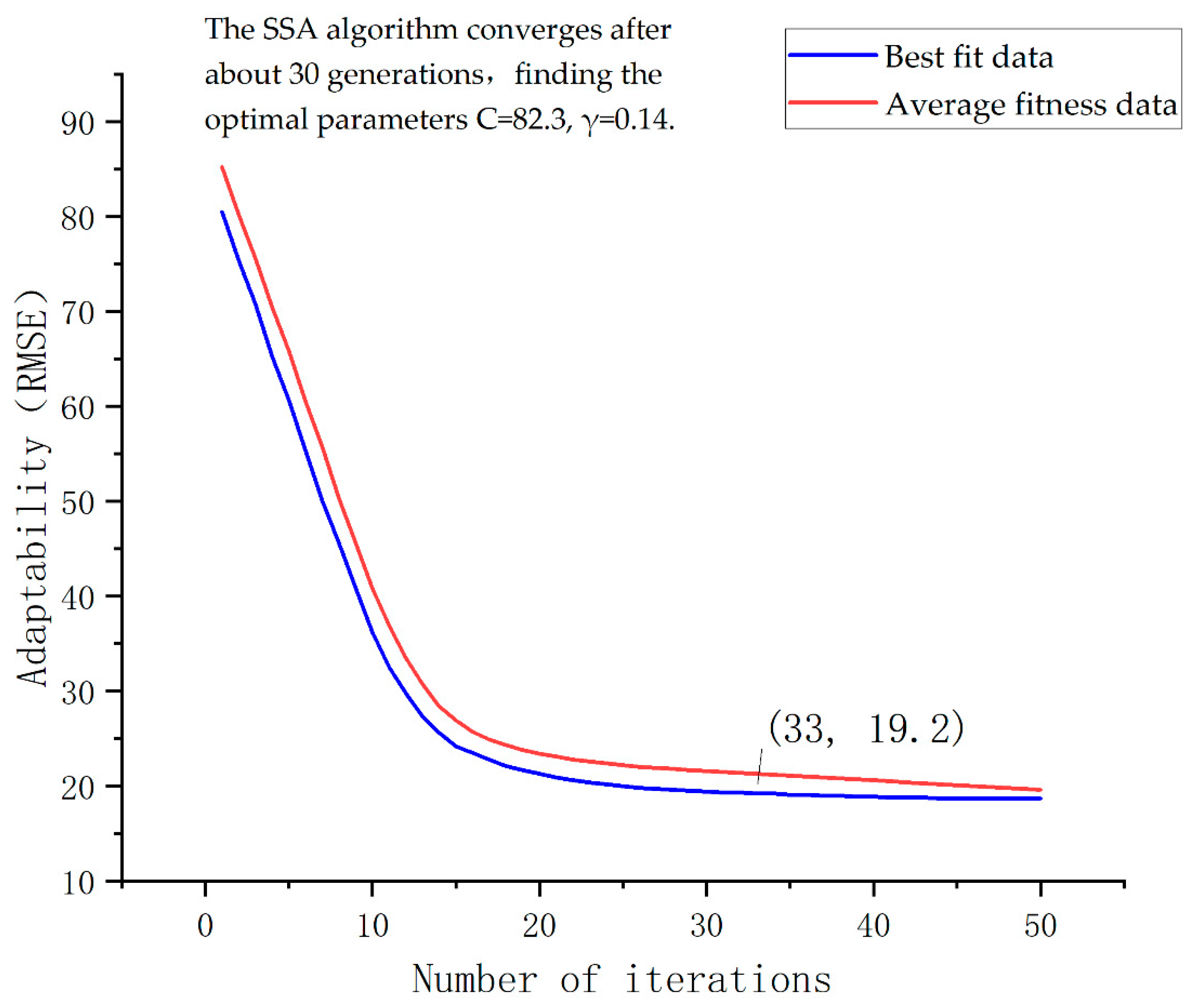
The process of optimizing the SVR parameters using Bayesian optimization is as follows: with the goal of minimizing the fitness function (i.e., the root mean square error of SVR on the validation set), the parameter search range is set to C ∈ [0.1, 100], γ ∈ [0.001, 10]. The Bayesian optimization uses a Gaussian process as the surrogate model and expected improvement (EI) as the acquisition function, with the number of initial points set to 10 and the number of iterations set to 50. As shown in Figure 9, the algorithm converges to the global optimal solution after about 30 iterations, and finally obtains the optimal parameter combination C = 85.7 and γ = 0.12. The parameters in this group significantly improve the ability of SVR to capture the nonlinear relationship in the landslide displacement sequence, and the RMSE of the validation set decreases by about 28.3% compared with the default parameters.
The parameter settings of the remaining models take into account both performance and efficiency: the number of trees set in the XGBoost model is Ntrees = 200, the learning rate η = 0.1, the maximum depth d = 6, the subsample rate ρ = 0.8, and the L2 regularization coefficient λ = 1.2 to balance the complexity of the model and the generalization ability. The number of trees in the random forest (RF) is set as Ntrees = 500, the minimum number of samples in the nodes is nmin = 5, and the feature selection strategy is the square root rule to give full play to its integration advantages. The time convolutional network (TCN) uses four residual blocks, the expansion factor δ = 2, the convolutional kernel size k = 3, and the dropout rate is set to 0.2 to alleviate overfitting and enhance the temporal feature extraction ability. All continuous numerical features are normalized to eliminate dimensional effects and accelerate model convergence.
SVR: Bayesian optimization was used to optimize the kernel function parameters, with the search range C 0.1 , 100 , γ 0.001 , 10 , and the optimal parameters C = 82.3, γ = 0.14 after 50 iterations.
XGBoost model: learning rate η = 0.1 , maximum tree depth d = 6 , subsample rate ρ = 0.8 , regularization parameter η = 1.2 , number of iterations N t r e e s = 200 t r e e s .
TCN: expansion factor δ = 2 , convolutional kernel size k = 3 , residual block number N = 4 , dropout rate = 0.2.
Random forest model: number of trees N t r e e s = 500 t r e e s , minimum number of nodes N min = 5 , number of feature selections m = n.

5.1.3. Stacking Fusion Mechanism

The stacking fusion mechanism adopts a dynamic weighting strategy, and the weight allocation of the base model comprehensively considers its prediction error (RMSE) and stability (prediction variance), and ensures that the sum of weights is 1 through normalization processing. The formula for defining weights is as follows:
w i = α 1 / R M S E i j = 1 n 1 / R M S E i + 1 α 1 / V a r i j = 1 n 1 / V a r
where R M S E i is the root mean square error of the ith base model in the validation set, and V a r i is the variance of the prediction results of the ith base model in the validation set; α is the accuracy–stability balance factor, to determine the optimal value through grid search, and n is the total number of base models.
Time series cross-validation: The training set window is 48 periods (December 2006–November 2010), and the validation set window is 12 periods (December 2010–December 2011).
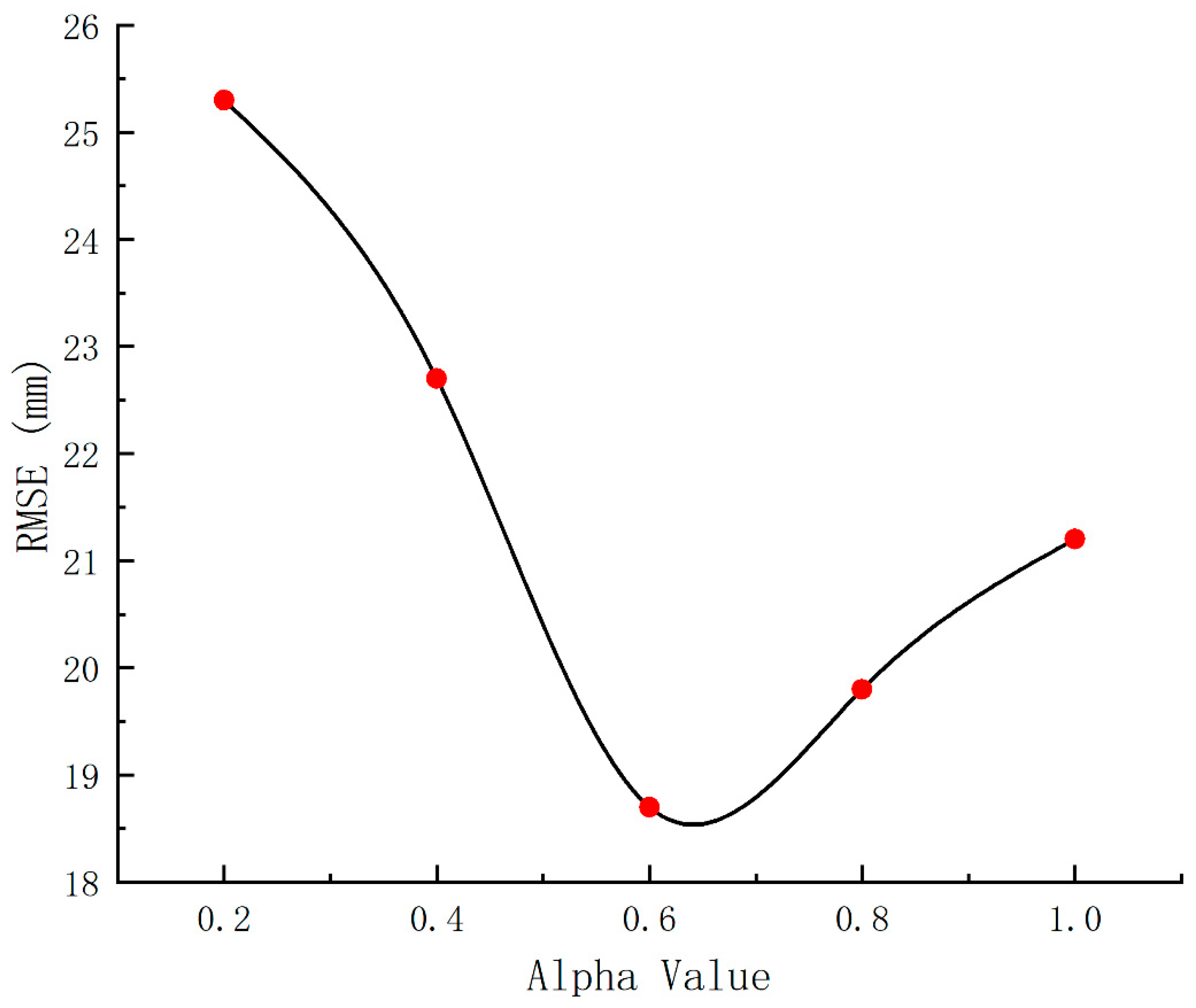
Balance factor α tuning: Set the α search range {0.0, 0.2, 0.6, 0.8, 1.0}, and select the value that makes the integration model RMSE the smallest in the validation set, where α = 0.6. The performance curve of the Alpha parameter is shown in Figure 10. The weight distribution is shown in Table 2.

5.2. Forecast Results and Analysis

5.2.1. Model Performance Indicators

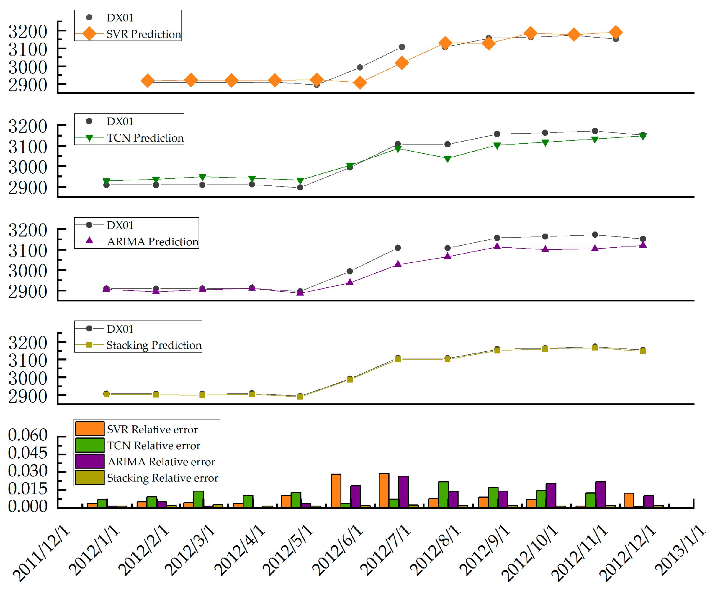
The model evaluation indicators and predictions of the stacking model and the base model at the XD-01 monitoring point are shown in Table 3 and Figure 9:
The results show that the stacking fusion model shows excellent prediction performance at the XD-01 monitoring point (Table 3). Its R2 = 0.9613 is significantly higher than that of the single model, indicating that the model can explain 96.13% of the displacement variation. The RMSE and MAE were 18.73 mm and 19.23 mm, respectively, which were 38.0% and 37.6% lower than those of the optimal single model (XGBoost), indicating that the fusion model had obvious advantages in point prediction accuracy.
The Baishui River landslide is a sedimentary layer landslide, and the sliding body is mainly composed of silty clay and gravel soil, with poor permeability, and heavy rainfall can easily lead to a sudden increase in pore water pressure and cause sudden displacement changes. The stacking model significantly increases the weights of the TCN and XGBoost in rainfall events through a dynamic weighting mechanism, and enhances the response ability to mutation signals.

5.2.2. Comparison of Prediction Curves

As can be seen from Figure 4, the prediction error of the stacking model for the sudden displacement change (from 2188.6 mm to 2208.3 mm) in the heavy rainfall event in July 2011 (rainfall of 237.3 mm) is less than 5%, while both the SVR and TCN lag or underestimate. This shows that the fusion model can better couple the rainfall–displacement response mechanism and is suitable for the prediction of hydrodynamic pressure landslides in the Three Gorges Reservoir area.

5.3. Comparative Experiments and Discussions

The stacking model is compared with the traditional SVR, TCN, and ARIMA models, and the results are shown in Table 4 and Figure 11.
Stacking outperformed the comparison model on R2, RMSE, and MAE. Its RMSE is 51.2% lower than the TCN and 54.4% lower than ARIMA, indicating that ensemble learning can effectively integrate the advantages of different models and improve prediction stability.
The ARIMA model assumes that the time series is linear and stationary, and it is difficult to capture the non-stationary mutation of landslide displacement. Although a TCN can capture long-term dependence, it does not respond well to short-term mutations. Stacking relies on XGBoost and RF in the stationary period and a TCN and SVR in the mutation period through dynamic weighting mechanisms to achieve multi-mechanism collaborative prediction.

6. Conclusions

6.1. Research Conclusions

This study addresses the issues of the insufficient accuracy and weak generalization of a single model in landslide displacement prediction, and proposes a machine learning ensemble prediction model based on dynamic weight stacking. Through case validation on the Baishui River landslide in the Three Gorges Reservoir area, the following main conclusions were drawn:
(1)
A high-precision dynamic fusion framework was proposed as follows: by introducing a dynamic weight allocation mechanism centered on prediction accuracy (RMSE) and stability (variance), and setting an accuracy–stability balance coefficient (α = 0.6), an adaptive weighted stacking model was successfully constructed. This framework effectively addresses the lag in response of traditional static fusion methods during displacement mutation periods, significantly enhancing the predictive model’s adaptability to complex working conditions.
(2)
The model’s excellent predictive performance has been validated: in an empirical study of a typical stacked-layer landslide (Baishui River landslide), the hybrid model demonstrated a significant advantage. On the test set at monitoring point XD-01, its R2 reached 0.9613, approximately 6.5% higher than the best single model (XGBoost); its RMSE (18.73 mm) and MAE (19.23 mm) decreased by 51.2% and 42.0%, respectively, compared to the TCN model. Notably, the model accurately captured the displacement surge (ΔF = 125.3 mm) triggered by heavy rainfall in July 2011, with an error of less than 5%, fully demonstrating the strong capability of multi-model collaboration in characterizing complex displacement trends and abrupt changes.
(3)
Effectively complementing the advantages of heterogeneous models: This stacking framework organically integrates the anti-overfitting characteristics of SVR, XGBoost, TCN, and random forest. This “ensemble of ensembles” strategy provides a more reliable technical tool for monthly-scale landslide disaster early warning in the Three Gorges Reservoir area.

6.2. Practical Application Challenges and Prospects

Although this study has achieved good results in model accuracy, integrating it successfully into actual landslide monitoring and early warning systems still faces several challenges, which is also an important direction for future research:
(1)
Real-time data and quality assurance: Model performance depends on high-quality, real-time displacement and rainfall data streams. In practical applications, it is necessary to establish stable and reliable automated monitoring and data transmission links, and to develop more robust algorithms to cope with more frequent data loss and noise in field environments.
(2)
Model generalization and data diversity: This study validated the effectiveness of the model using a single landslide case in the Baishui River. An important direction for future work is to incorporate more landslide cases with different geomechanical conditions and longer-term monitoring data to further verify and enhance the model’s generality and robustness.

Author Contributions

Conceptualization, H.W., A.H. and Y.L.; methodology, H.W. and Y.L.; validation, H.W., A.H., Y.W. and D.Q.; formal analysis, Y.L. and Y.W.; investigation, H.W., Y.L. and D.Q.; resources, A.H. and D.Q.; data curation, Y.W. and Y.L.; writing—original draft preparation, H.W. and Y.L.; writing—review and editing, A.H. and D.Q.; visualization, Y.W.; supervision, A.H.; project administration, A.H.; funding acquisition, H.W. and A.H. All authors have read and agreed to the published version of the manuscript.

Funding

China Railway Group Limited Science and Technology Research and Development Plan Project (2022-Major Project-07); Gansu Province Technology Innovation Guidance Program—Special Project for the Capacity Building of Enterprise R&D Institutions (23CXJA0011); National Railway Administration Project (KF2025-077).

Data Availability Statement

The landslide displacement and rainfall data used in this study are publicly available at the National Cryosphere Desert Data Center (https://s.ncdc.ac.cn/portal/, accessed on 30 October 2024). The implemented algorithms and processing scripts can be requested from the corresponding author for reasonable purposes.

Conflicts of Interest

Authors Yongqiang Li, Yinsheng Wang and Honggang Wu were employed by the company China Railway Science Research Institute Group Co., Ltd. Yongqiang Li and Honggang Wu were employed by the company China Railway Northwest Scientific Research Institute Co., Ltd. The remaining authors declare that the research was conducted in the absence of any commercial or financial relationships that could be construed as a potential conflict of interest. The funders had no role in the design of the study; in the collection, analysis, or interpretation of data, in the writing of the manuscript, or in the decision to publish the result.

List of Abbreviations

SVRSupport vector regression
XGBoostExtreme gradient boosting
TCNTemporal Convolutional Network
RFRandom forest
RMSERoot mean square error
MAEMean absolute error

References

  1. Froude, M.J.; Petley, D.N. Global fatal landslide occurrence from 2004 to 2016. Nat. Hazards Earth Syst. Sci. 2018, 18, 2161–2181. [Google Scholar] [CrossRef]
  2. Miao, H.B.; Wang, G.H.; Yin, K.L.; Kamai, T.; Li, Y.Y. Mechanism of the slow-moving landslides in jurassic red-strata in the three gorges reservoir, china. Eng. Geol. 2014, 171, 59–69. [Google Scholar] [CrossRef]
  3. Petley, D. Global patterns of loss of life from landslides. Geology 2012, 40, 927–930. [Google Scholar] [CrossRef]
  4. Tang, H.M.; Wasowski, J.; Juang, C.H. Geohazards in the three gorges reservoir area, china lessons learned from decades of research. Eng. Geol. 2019, 261, 105267. [Google Scholar] [CrossRef]
  5. Wang, Y.K.; Tang, H.M.; Huang, J.S.; Wen, T.; Ma, J.W.; Zhang, J.R. A comparative study of different machine learning methods for reservoir landslide displacement prediction. Eng. Geol. 2022, 298, 106544. [Google Scholar] [CrossRef]
  6. Guzzetti, F.; Mondini, A.C.; Cardinali, M.; Fiorucci, F.; Santangelo, M.; Chang, K.T. Landslide inventory maps: New tools for an old problem. Earth-Sci. Rev. 2012, 112, 42–66. [Google Scholar] [CrossRef]
  7. Merghadi, A.; Yunus, A.P.; Dou, J.; Whiteley, J.; ThaiPham, B.; Bui, D.T.; Avtar, R.; Abderrahmane, B. Machine learning methods for landslide susceptibility studies: A comparative overview of algorithm performance. Earth-Sci. Rev. 2020, 207, 103225. [Google Scholar] [CrossRef]
  8. Goetz, J.N.; Brenning, A.; Petschko, H.; Leopold, P. Evaluating machine learning and statistical prediction techniques for landslide susceptibility modeling. Comput. Geosci. 2015, 81, 1–11. [Google Scholar] [CrossRef]
  9. Stumpf, A.; Kerle, N. Object-oriented mapping of landslides using random forests. Remote Sens. Environ. 2011, 115, 2564–2577. [Google Scholar] [CrossRef]
  10. Yue, Y.G.; Cao, L.; Lu, D.W.; Hu, Z.Y.; Xu, M.H.; Wang, S.X.; Li, B.; Ding, H.H. Review and empirical analysis of sparrow search algorithm. Artif. Intell. Rev. 2023, 56, 10867–10919. [Google Scholar] [CrossRef]
  11. Yan, S.Q.; Liu, W.D.; Li, X.Q.; Yang, P.; Wu, F.X.; Yan, Z. Comparative study and improvement analysis of sparrow search algorithm. Wirel. Commun. Mob. Comput. 2022, 2022, 4882521. [Google Scholar] [CrossRef]
  12. Emmanuel, T.; Mpoeleng, D.; Maupong, T. Power plant induced-draft fan fault prediction using machine learning stacking ensemble. J. Eng. Res. 2024, 12, 82–90. [Google Scholar] [CrossRef]
  13. Webb, G.I.; Zheng, Z.J. Multistrategy ensemble learning: Reducing error by combining ensemble learning techniques. IEEE Trans. Knowl. Data Eng. 2004, 16, 980–991. [Google Scholar] [CrossRef]
  14. Ganaie, M.A.; Hu, M.H.; Malik, A.K.; Tanveer, M.; Suganthan, P.N. Ensemble deep learning: A review. Eng. Appl. Artif. Intell. 2022, 115, 105151. [Google Scholar] [CrossRef]
  15. Drucker, H.C.; Burges, C.J.C.; Kaufman, L.; Smola, A.; Vapnik, V. Support vector regression machines. Adv. Neural Inf. Process. Syst. 1997, 9, 155–161. [Google Scholar]
  16. Brereton, R.G.; Lloyd, G.R. Support vector machines for classification and regression. Analyst 2010, 135, 230–267. [Google Scholar] [CrossRef]
  17. Wu, C.H.; Ho, J.M.; Lee, D.T. Travel-time prediction with support vector regression. IEEE Trans. Intell. Transp. Syst. 2004, 5, 276–281. [Google Scholar] [CrossRef]
  18. Smola, A.J.; Schölkopf, B. On a kernel-based method for pattern recognition, regression, approximation, and operator inversion. Algorithmica 1998, 22, 211–231. [Google Scholar] [CrossRef]
  19. Chen, T.Q.; Guestrin, C. Xgboost: A scalable tree boosting system. In Proceedings of the 22nd Acm Sigkdd International Conference on Knowledge Discovery and Data Mining (Kdd’16), New York, NY, USA, 13–17 August 2016; pp. 785–794. [Google Scholar] [CrossRef]
  20. Friedman, J.H. Stochastic gradient boosting. Comput. Stat. Data Anal. 2002, 38, 367–378. [Google Scholar] [CrossRef]
  21. Lea, C.; Vidal, R.; Reiter, A.; Hager, G.D. Temporal convolutional networks: A unified approach to action segmentation. In Computer Vision—Eccv 2016 Workshops; Springer: Cham, Switzerland, 2016; Volume 9915, pp. 47–54. [Google Scholar] [CrossRef]
  22. Victoria, A.H.; Maragatham, G. Automatic tuning of hyperparameters using bayesian optimization. Evol. Syst. 2021, 12, 217–223. [Google Scholar] [CrossRef]
  23. Alibrahim, H.; Ludwig, S.A. Hyperparameter optimization: Comparing genetic algorithm against grid search and bayesian optimization. In Proceedings of the 2021 IEEE Congress on Evolutionary Computation (Cec 2021), Kraków, Poland, 28 June–1 July 2021; pp. 1551–1559. [Google Scholar] [CrossRef]
  24. Breiman, L. Random forests. Mach. Learn. 2001, 45, 5–32. [Google Scholar] [CrossRef]
  25. Wolpert, D.H. Stacked generalization. Neural Netw. 1992, 5, 241–259. [Google Scholar] [CrossRef]
  26. Naimi, A.I.; Balzer, L.B. Stacked generalization: An introduction to super learning. Eur. J. Epidemiol. 2018, 33, 459–464. [Google Scholar] [CrossRef]
Figure 1. Structure of support vector regression (SVR) for regression prediction.
Applsci 15 11747 g001
Figure 2. Architecture of the Temporal Convolutional Network (TCN).
Applsci 15 11747 g002
Figure 3. Structure of the random forest (RF) model.
Applsci 15 11747 g003
Figure 4. Framework of the stacking-based ensemble learning method.
Applsci 15 11747 g004
Figure 5. Workflow of the landslide displacement prediction method based on multi-model fusion under the stacking framework.
Applsci 15 11747 g005
Figure 6. Original GPS monitoring data of landslide displacement at points ZG118 and XD-01.
Applsci 15 11747 g006
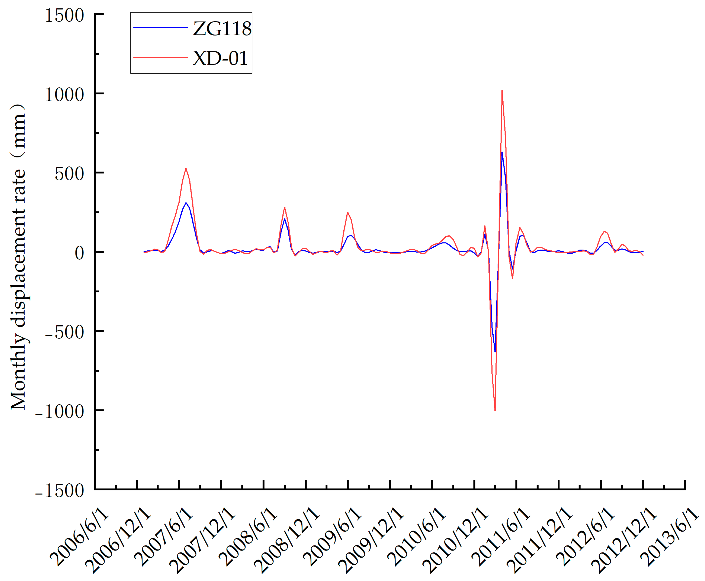
Figure 7. Monthly displacement rate chart.
Applsci 15 11747 g007
Figure 8. Cumulative landslide displacement and rainfall monitoring curves after preprocessing for points ZG118 and XD-01.
Applsci 15 11747 g008
Figure 9. Bayesian optimization convergence curve for SVR hyperparameter tuning.
Applsci 15 11747 g009
Figure 10. Alpha parameter performance curve chart.
Applsci 15 11747 g010
Figure 11. Comparison chart of predictions from multiple models.
Applsci 15 11747 g011
Table 1. Corrected part of the data table.
TimeZG118XD-1Rainfall
2010/112076.42710.512.9
2010/122069.22731.69.4
2011/12073.42731.514.5
2011/22069.72715.738.4
2011/32068.62723.836.9
2011/42067.42731.8106.7
2011/52070.12696.6190.7
Table 2. Base model weight allocation table.
Base ModelRMSE (mm)Variance (mm3)wi (a = 0.6)
SVR42.555.00.16
XGBoost30.225.30.34
RF34.832.70.24
TCN31.528.90.26
Table 3. Comparison and analysis table with single-model prediction.
ModelR2RMSE (mm)MAE (mm)
SVR0.874340.898630.8392
TCN0.845738.456533.1624
Stacking0.961318.732919.2326
Table 4. Comparison and analysis table with traditional model prediction results.
ModelR2RMSE (mm)MAE (mm)
SVR0.874340.898630.8392
ARIMA0.868541.085832.0194
TCN0.845738.456533.1624
Stacking0.961318.732919.2326
Disclaimer/Publisher’s Note: The statements, opinions and data contained in all publications are solely those of the individual author(s) and contributor(s) and not of MDPI and/or the editor(s). MDPI and/or the editor(s) disclaim responsibility for any injury to people or property resulting from any ideas, methods, instructions or products referred to in the content.