ESSTformer: A CNN-Transformer Hybrid with Decoupled Spatial Spectral Transformers for Hyperspectral Image Super-Resolution

Abstract

Hyperspectral images (HSIs) are crucial for ground object classification, target detection, and related applications due to their rich spatial spectral information. However, hardware limitations in imaging systems make it challenging to directly acquire HSIs with a high spatial resolution. While deep learning-based single hyperspectral image super-resolution (SHSR) methods have made significant progress, existing approaches primarily rely on convolutional neural networks (CNNs) with fixed geometric kernels, which struggle to model global spatial spectral dependencies effectively. To address this, we propose ESSTformer, a novel SHSR framework that synergistically integrates CNNs’ local feature extraction and Transformers’ global modeling capabilities. Specifically, we design a multi-scale spectral attention module (MSAM) based on dilated convolutions to capture local multi-scale spatial spectral features. Considering the inherent differences between spatial and spectral information, we adopt a decoupled processing strategy by constructing separate spatial and Spectral Transformers. The Spatial Transformer employs window attention mechanisms and an improved convolutional multi-layer perceptron (CMLP) to model long-range spatial dependencies, while the Spectral Transformer utilizes self-attention mechanisms combined with a spectral enhancement module to focus on discriminative spectral features. Extensive experiments on three hyperspectral datasets demonstrate that the proposed ESSTformer achieves a superior performance in super-resolution reconstruction compared to state-of-the-art methods.

1. Introduction

Hyperspectral images (HSIs) capture the reflectance or transmittance information of objects across dozens to hundreds of continuous spectral bands. Compared with standard natural images, HSIs possess more spectral bands, which enables them to acquire richer spectral detail information that more accurately characterizes the fine features and intrinsic properties of objects. Consequently, hyperspectral imaging has been widely applied in numerous fields including remote sensing [1,2,3], medical imaging [4,5,6], and industrial inspection [7,8,9]. However, constrained by imaging mechanisms and equipment limitations, acquired hyperspectral images require tradeoffs among spatial resolution, spectral resolution, swath width, and signal-to-noise ratio, making it difficult to directly obtain high-spatial-resolution hyperspectral images. Yet, in application scenarios such as mineral exploration [10], urban fine-scale mapping [11], and small target detection [12], a higher spatial resolution is essential. This limited spatial resolution has become a bottleneck restricting hyperspectral imaging applications in remote sensing technology. Although hardware improvements can enhance resolution, such approaches often involve high costs and lengthy cycles. In comparison, image processing techniques for resolution enhancement offer greater practical value.

Super-resolution (SR) [13] technology enables the reconstruction of high-resolution images consistent with the original scene from either a single or a sequence of low-resolution images. For hyperspectral image super-resolution reconstruction, a key classification hinges on whether auxiliary information (e.g., panchromatic images [14,15], RGB images [16,17], or multispectral images [18]) is employed; this divides the methods into two main categories, namely fusion-based hyperspectral image super-resolution and single image hyperspectral super-resolution (SHSR). The fusion-based approach enhances the spatial resolution of the target hyperspectral image by fusing low-resolution hyperspectral images with high-resolution auxiliary images. However, this method relies on a critical assumption involving a perfect registration between the low-resolution hyperspectral images and the high-resolution auxiliary images. In practical scenarios, acquiring high-quality auxiliary images is often challenging, if not entirely unfeasible. In contrast, SHSR requires no auxiliary information throughout the reconstruction process. It can yield satisfactory performance in most cases, thereby demonstrating a broad application potential.

SHSR methods can be primarily categorized into traditional approaches and deep learning-based methods. Most traditional methods, such as those based on sparse representation [19,20] and low-rank matrices [21,22], typically rely on manually designed prior knowledge (e.g., self-similarity, sparsity, and low-rank properties) as regularization terms to guide the reconstruction process. While these methods can deliver relatively favorable results in specific scenarios, their reliance on handcrafted priors gives rise to two key limitations, manifesting in computationally intensive processes and constrained representation capability. These drawbacks further restrict their ability to fully capture the inherent characteristics of hyperspectral data. With the rapid advancement of deep learning techniques, especially the widespread adoption of convolutional neural networks (CNNs), deep learning-based SHSR methods have achieved remarkable performance breakthroughs [23,24]. Nevertheless, due to the fixed size of their convolutional kernels, CNNs inherently possess limited receptive fields, which renders them inefficient in modeling long-range dependencies. Additionally, most of these CNN-based methods only focus on single-scale spatial features of HSIs, while overlooking the rich multi-scale mapping relationships across multi-scale spaces. This oversight ultimately limits the further improvement of their overall reconstruction performance [25].

In recent years, Transformer models [26] have been successfully applied to HSI classification tasks, owing to their exceptional ability to capture global information. However, hyperspectral datasets typically have a limited number of training samples, which poses a particular challenge for training effective Transformer models for SR tasks. Furthermore, research on Transformer architectures specifically tailored to SR remains relatively scarce. To address the limitation of Transformers struggling with small-scale datasets, several studies have attempted to integrate CNNs with Transformers [27,28,29]. For example, Interactformer [28] adopts a hybrid architecture that combines 3D convolutions with Transformer modules, enabling the simultaneous extraction of local and global spatial spectral features. Nevertheless, the extensive use of 3D convolutions and parallel structures leads to a high computational complexity, as well as increased demands on hardware memory resources.

The Enhanced Spatial Spectral Transformer (ESSTformer) is proposed for SHSR to address these challenges. This novel framework innovatively integrates the strengths of CNNs and Transformer architectures, achieving significant improvements in reconstruction performance by synergistically extracting local and global spatial spectral features. For local feature extraction, we design a multi scale spectral attention module (MSAM) based on dilated convolutions. This module captures multi-scale spatial features via its dilated convolution design, while leveraging a spectral attention mechanism to dynamically adjust weights across different spectral bands, enabling the more effective extraction of local spatial spectral information. For global feature modeling, we adopt a decoupled processing strategy that separately constructs spectral and Spatial Transformers to better handle the distinct characteristics of these modalities. In the Spectral Transformer, inter-band correlations are preserved through self-attention mechanisms, and a spectral enhancement module is introduced to dynamically adjust inter-band weights, which emphasizes critical spectral information and enables the more accurate selection and fusion of important spectral features, thus improving the spectral fidelity of reconstructed images. In the Spatial Transformer, windowed attention is employed to model long-range spatial dependencies, while a locally enhanced feed-forward network maintains essential local neighborhood information. This design simultaneously preserves spatial details and mitigates the excessive computational costs associated with standard self-attention. Comprehensive qualitative and quantitative experiments across three hyperspectral datasets demonstrate the effectiveness of the ESSTformer. Our main contributions are summarized as follows:

• We propose ESSTformer, a novel CNN-Transformer hybrid framework for SHSR that effectively exploits both local and global spatial spectral information, significantly boosting the super-resolution performance.
• We design the MSAM to learn multi-scale interactions between local spatial and spectral features, substantially enhancing the local feature representation.
• Considering the inherent differences between spatial and spectral characteristics, we develop a decoupled processing strategy with dedicated Transformer modules; the Spatial Transformer captures global spatial dependencies while the Spectral Transformer models long-range spectral relationships, working synergistically to improve feature extraction precision.
• We replace standard MLPs with convolutional multi-layer perceptrons (CMLPs) to better leverage neighborhood spatial context, thereby enhancing the model’s representational capacity and adaptability.

2. Materials and Methods

In this section, we present a detailed description of the proposed SHSR method, ESSTformer, which is structured around five essential components: the overall framework, MSAM, the Spectral Transformer, the Spatial Transformer and the loss function.

2.1. Overall Framework

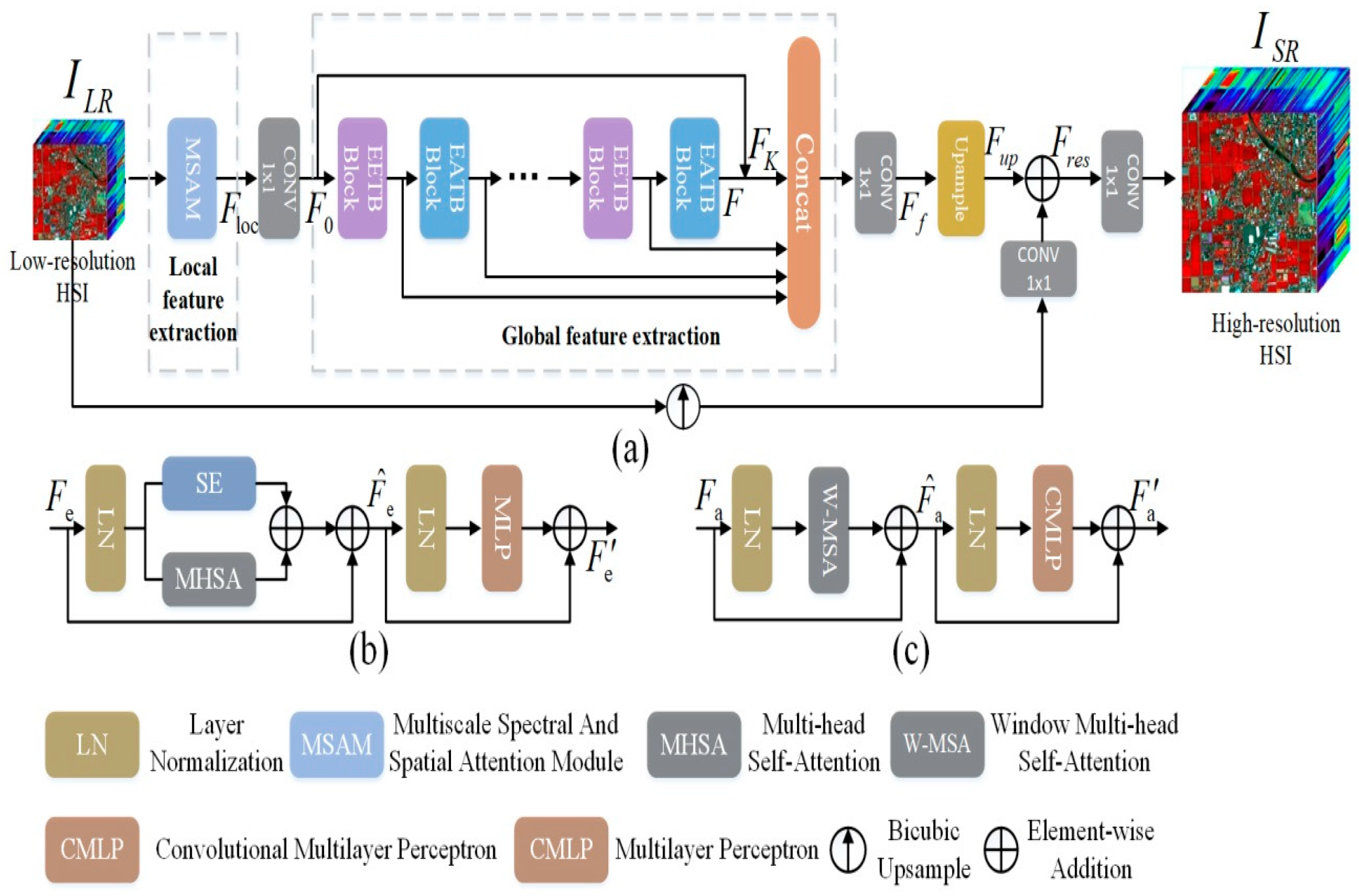
As illustrated in Figure 1, the proposed ESSTformer model in this paper combines CNNs and Transformer architectures to simultaneously process both local and global spatial spectral information of hyperspectral images. The model takes a low-resolution hyperspectral image $I_{LR}\in R^{H\times W\times B}$ with dimensions $H\times W\times B$ (where $H$, $W$, and $B$ denote the height, width, and number of spectral as input, and outputs a high-resolution hyperspectral image $I_{SR}\in R^{\mathrm{s}H\times sW\times B}$ with a super-resolution scale factor of s. The objective of the ESSTformer network is to predict the super-resolved image ISR from the input low-resolution image ILR, making it as close as possible to the original high-resolution hyperspectral image $I_{HR}\in R^{\mathrm{s}H\times sW\times B}$, which can be expressed as follows:

$$I_{SR}=H_{ESSTformer}(I_{LR}),$$

(1)

where $H_{ESSTformer}(\cdot )$ represents the function corresponding to the proposed ESSTformer methodology.

For the purpose of extracting local spatial spectral information, we designed the MSAM to capture features across different scales. The module can be formally expressed as follows:

$$F_{\mathrm{loc}}=H_{MSAM}(I_{LR}),$$

(2)

where $F_{loc}$ represents the extracted local spatial spectral features, and $H_{MSAM}(\cdot )$ denotes the function corresponding to the operation of the MSAM applied to the input $I_{LR}$.

For the full exploitation of global spatial spectral information, we first project the extracted local features $F_{loc}$ into the hyperspectral dimension, which can be represented as follows:

$$F_0=H_0(F_{loc}),$$

(3)

where $F_0\in R^{H\times W\times B}$ represents the hyperspectral spatial spectral features with C spectral bands, $H\times W$ denotes the spatial resolution, and $H_0(\cdot )$ refers to the 1 × 1 convolutional function.

The extracted features $F_0$ are then fed into an Enhanced Spectral Transformer Block (EETB) to model inter-band correlations across different spectral wavelengths, thereby capturing global spectral characteristics. Subsequently, the feature maps output from the EETB module are processed by an Enhanced Spatial Transformer Block(EATB) to establish long-range dependencies in the spatial dimension. We construct multiple cascaded EETB and EATB modules to comprehensively extract both spatial and spectral features. The output feature map F from the final EATB module is fused with feature map $F_0$ obtained through long skip connections, generating a new feature representation $F_K$. To prevent the loss of low-frequency information, we employ residual connections by concatenating each module’s output with $F_K$, followed by a 1 × 1 convolution for dimensionality reduction to ensure feature map $F_f$ maintains the same dimensions as F. Finally, an upsampling module expands the spatial resolution of the fused deep spatial spectral features $F_f$, which can be formally expressed as follows:

$$F_{up}=H_{up}(F_f),$$

(4)

where $H_{up}(\cdot )$ denotes the upsampling function based on the Pixel Shuffle technique [30], and $F_{\mathrm{up}}$ has C spectral bands with spatial dimensions of $sH\times sW$. Through this series of processing steps, the feature map is significantly enhanced in both spectral representation and spatial resolution, leading to a richer, multi-dimensional feature map that effectively captures the global spatial and spectral context of the input data.

Finally, bicubic interpolation is applied to upsample the input features, mitigating training complexity and helping to preserve original information through subsequent residual connections to the network’s output. After bicubic interpolation, a 1 × 1 convolutional layer is used to adjust the spatial dimensions of the interpolated feature map, ensuring it aligns with the output feature dimensions $F_f$, thus generating the residual feature $F_{res}$. To maintain the spatial resolution of the final reconstructed image, consistent with the original high-resolution hyperspectral image, an additional 1 × 1 convolutional layer is applied to the feature map $F_{res}$, which has already been adjusted by both interpolation and convolution. The upsampling process can be formalized as follows:

$$F_{res}=F_{up}+H_1(I_{LR}\uparrow ),$$

(5)

$$I_{SR}=H_2(F_{res}),$$

(6)

where $F_{res}\in R^{sH\times sW\times C}$ represents the residual feature, $H_1(\cdot )$ and $H_2(\cdot )$ denote the 1 × 1 convolutional layers, $I_{LR}\uparrow$ is the bicubic upsampled version of the input low-resolution hyperspectral image, and $I_{SR}$ is the reconstructed high-resolution hyperspectral image.

2.2. MSAM

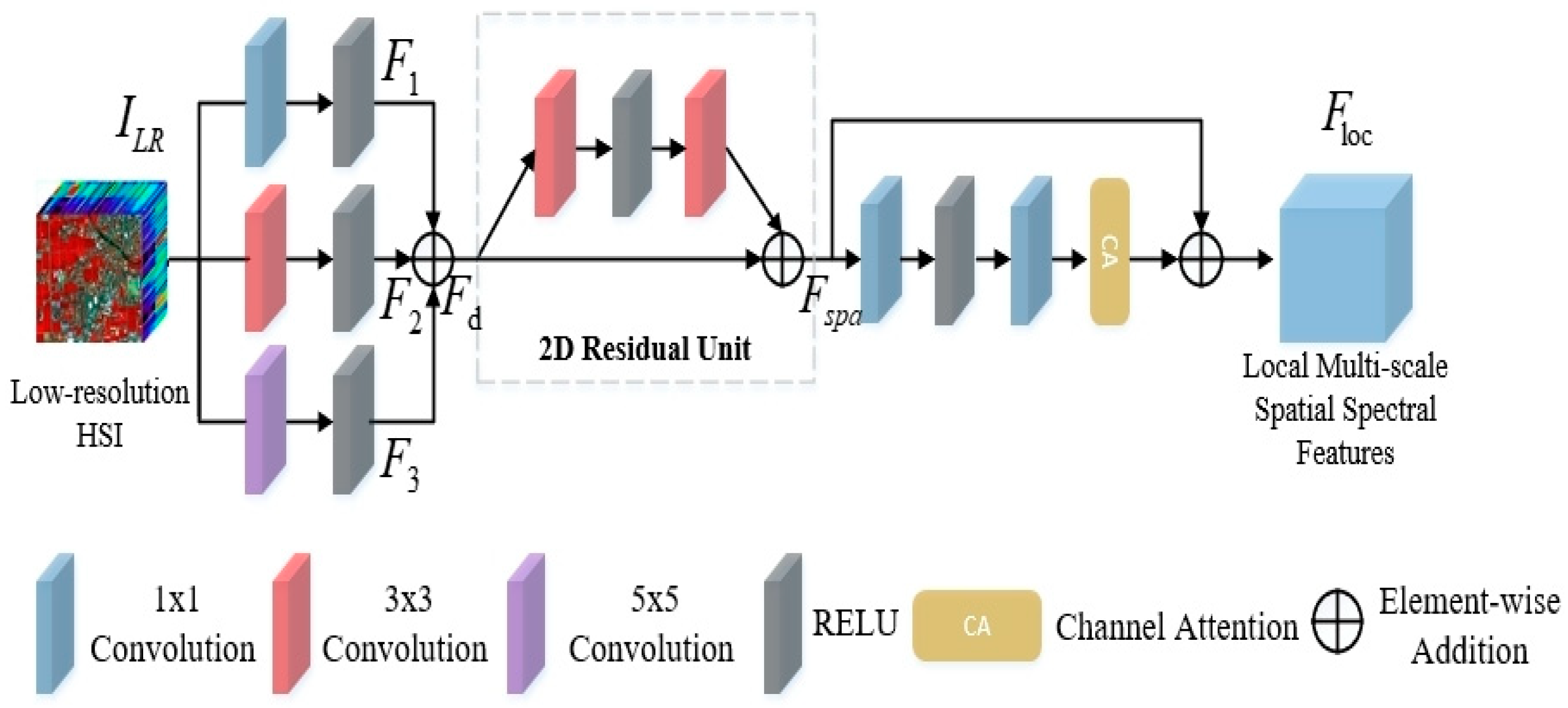
Currently, most SHSR methods primarily rely on 2D or 3D convolutions to extract spatial spectral features at a single scale, which inherently limits the model’s ability to explore rich scale-wise mapping relationships in multi-scale spaces. The MSAM, illustrated in Figure 2, is designed to address this limitation by capturing local multi-scale spatial spectral features of the image.

While existing methods often rely on convolutional kernels of fixed receptive fields, their capacity to represent multi-scale spatial spectral contexts remains limited. Accordingly, we design the MSAM, aimed at explicitly capturing local features at multiple scales. The module takes $I_{LR}$ as input. Specifically, we employ dilated convolutions with three distinct dilation rates (1, 3, 5), combined with ReLU activation functions, to capture multi-scale spatial information. The extracted features $F_i$ at each scale are expressed as follows:

$$F_1=H_D(I_{LR},1),$$

(7)

$$F_2=H_D(I_{LR},2),$$

(8)

$$F_3=H_D(I_{LR},3),$$

(9)

where $H_D(\cdot ,\cdot )$ represents the dilated convolution function. Subsequently, the multi-scale features $F_i$ extracted at different scales are fused and further refined through a Residual Spatial Module to obtain residual multi-scale spatial features $F_{spa}$, which can be formally expressed as follows:

$$F_d=F_1+F_2+F_3,$$

(10)

$$F_{spa}=F_d+H_3(F_d),$$

(11)

where $H_3(\cdot )$ represents the composite function of two 3 × 3 convolutional layers (with intermediate RELU activation) in the Residual Spatial Module. A Residual Channel Attention Block (RCAB) [31] is incorporated to enhance the representation by modeling inter-band dependencies. The process is formally expressed as follows:

$$F_{loc}=H_{RCAB}(F_{spa}),$$

(12)

where $F_{loc}$ represents the local multi-scale spatial spectral features and $H_{RCAB}(\cdot )$ denotes the RCAB operation function.

Through MSAM processing, we successfully extract local multi-scale spatial spectral features from HSIs, while establishing a robust foundation for subsequent global spatial spectral feature extraction.

2.3. EETB

The strong inter-band spectral correlations in HSIs are particularly crucial for SHSR analysis. Therefore, to effectively capture these long-range dependencies between different spectral bands, we have designed the EETB module as shown in Figure 1b. The EETB module consists of two residual blocks, the first containing a Layer Normalization (LN) layer followed by a deformable convolution-based self-attention layer integrated with a spectral enhancement (SE) module to enhance feature representation capability, and the second comprising a LN layer with a subsequent MLP layer designed to deeply explore non-linear feature relationships. Let $F_e\in R^{H\times W\times C}$ represent the input to a single EETB module; the processing flow can be mathematically expressed as follows:

$${\widehat{F}}_{\mathrm{e}}=MHSA(LN(F_e))+SE(LN(F_e))+F_e,$$

(13)

$$F_e^{\prime }=MLP(LN({\widehat{F}}_e))+{\widehat{F}}_e,$$

(14)

where ${\widehat{F}}_{\mathrm{e}}$ denotes the enhanced spectral features, $F_e^{\prime }$ represents the global spectral features output by the EETB module, LN(·) refers to the function implemented by the Layer Normalization (LN) layer, and MLP(·) denotes the function implemented by the MLP layer.

2.3.1. Long Self-Attention

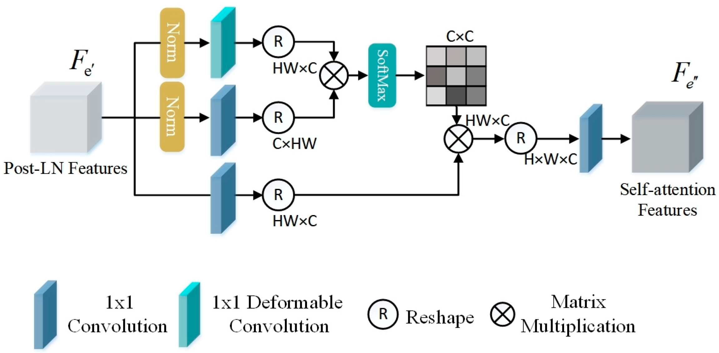
An adaptive multi-head self-attention mechanism is proposed to better capture correlations and variations among spectral bands. Its query ($Q$) is generated using deformable convolution, which allows the module to adaptively focus on more relevant spatial contexts based on input features, thereby achieving a more flexible receptive field than standard convolutions.

As illustrated in Figure 3, the normalized feature $F_{e^{\prime }}\in R^{H\times W\times C}$ is projected into query ($Q\in R^{H\times W\times C}$), key ($K\in R^{H\times W\times C}$), and value ($V\in R^{H\times W\times C}$) tensors. This projection process can be mathematically represented as follows:

$$Q=W_{deformable}(F_{e^{\prime }}),K=W_K(F_{e^{\prime }}),V=W_V(F_{e^{\prime }}),$$

(15)

where $W_{deformable}(\cdot )$ denotes the deformable convolution function, and $W_K(\cdot )$ and $W_V(\cdot )$ represent the 1 × 1 point-wise convolution functions.

Subsequently, the projected tensors are reshaped to $Q\in R^{HW\times C}$, $K\in R^{C\times HW}$, and $V\in R^{HW\times C}$, respectively, then split into N heads along the channel dimension. The attention mechanism for each head is computed as follows:

$$A\mathrm{tt}entio{n}_i(Q_i,K_i,V_i)=V_{i}SoftMax({\displaystyle \frac{Q_i{K}_{\mathrm{i}}^T}{\sqrt{d_k}}}),$$

(16)

where $d_k=C/N$ is the feature dimension per head. The outputs from all heads are concatenated and projected:

$$M\mathrm{u}ltiHead=Concat(Attentio{n}_1,Attentio{n}_2,\dots ,Attentio{n}_N),$$

(17)

Finally, the output is reshaped back to $H\times W\times C$ and processed by a 1 × 1 convolution to produce the enhanced spectral attentional features $F_{e^{″}}$. Our deformable attention mechanism effectively captures long-range spectral spatial dependencies through content-aware spatial sampling, significantly improving feature representation for SHSR tasks.

2.3.2. Spectral Enhancement

The SE module is incorporated to complement the spatial adaptive attention mechanism and further optimize the modeling of inter-channel dependencies. Designed as a computational unit for adaptive recalibration, it emphasizes informative spectral bands while suppressing less useful ones.

As illustrated in Figure 4, the input feature $F_{e^{\prime }}\in R^{H\times W\times C}$ is first squeezed into a channel descriptor vector $F_c\in R^{1\times 1\times C}$ via global average pooling. Subsequently, an excitation operation is applied through a simple gating mechanism with a sigmoid activation:

$$F_{\mathrm{z}}=\sigma (W_{\mathrm{h}}\delta (W_l{F}_c)),$$

(18)

where $\delta$ denotes the ReLU function, $W_{\mathrm{l}}\in R^{K\times C}$ and $W_{\mathrm{h}}\in R^{C\times K}$ are the weights of two linear layers forming a bottleneck structure for dimensionality reduction (K = C/r) and restoration, and $\sigma$ is the sigmoid function. The final output is obtained by scaling the original input with the computed channel weights:

$$F_{e^{‴}}=F_{e^{\prime }}\cdot F_z,$$

(19)

By explicitly modeling spectral channel relationships, this lightweight module ensures that subsequent processing stages focus on the most discriminative spectral features, thereby enhancing the overall representational capacity of our framework for hyperspectral image reconstruction.

2.4. EATB

While the EETB effectively models global inter-band correlations, its attention mechanism, which operates on flattened spectral vectors, is inherently limited in capturing long-range spatial dependencies. This is because the spectral self-attention prioritizes relationships between bands across all spatial locations but does not explicitly model the contextual relationships between different pixels or regions within the same band. Consequently, a standalone Spectral Transformer may struggle to reconstruct fine spatial structures and edges that require integrating information from distant parts of the image.

We advocate for a decoupled spatial spectral modeling strategy to address this fundamental limitation and achieve a more comprehensive representation. This design explicitly separates the learning of spectral and spatial features into dedicated Transformer blocks. Following the spectral feature extraction by the EETB, the EATB is introduced to explicitly and efficiently model long-range spatial contexts.

As shown in Figure 1c, the EATB module consists of two residual blocks: the first contains a LN followed by a window-based attention layer, while the second comprises an LN layer followed by a CMLP layer. Let $F_{\mathrm{a}}\in R^{H\times W\times C}$ be the input to a single EATB module; its processing can be expressed as follows:

$${\widehat{F}}_{\mathrm{a}}=WMSA(LN(F_a))+F_a,$$

(20)

$$F_a^{\prime }=CMLP(LN({\widehat{F}}_a))+{\widehat{F}}_a,$$

(21)

where ${\widehat{F}}_{\mathrm{a}}\in R^{H\times W\times C}$ represents the spatial features captured through the window attention mechanism, $F_a^{\prime }\in R^{H\times W\times C}$ denotes the global spatial features output by the EATB module, LN(·) refers to the operation function of the Layer Normalization layer, and CMLP(·) represents the operation function of the CMLP layer.

2.4.1. WMSA

The Window-based Multi-head Self-Attention (WMSA) module is adopted to efficiently model long-range spatial dependencies while avoiding the quadratic complexity of standard self-attention. The input feature map of size $H\times W\times C$ is first partitioned into non-overlapping $M\times M$ windows, reshaping the input to ${\displaystyle \frac{HW}{M^2}}\times M^2\times C$.

Within each window, the feature $F_{{\mathrm{a}}^{\prime }}\in R^{M\times M\times C}$ is projected into queries ($Q\in R^{M\times M\times C}$), keys ($K\in R^{M\times M\times C}$), and values ($V\in R^{M\times M\times C}$) via 1 × 1 convolutions:

$$Q=W_Q(F_{a^{\prime }}),K=W_K(F_{a^{\prime }}),V=W_V(F_{a^{\prime }}),$$

(22)

Subsequently, the projecte $Q$, $K$, and $V$ are reshaped into $Q\in R^{M^2\times C}$, $K\in R^{M^2\times C}$ and $V\in R^{M^2\times C}$, respectively. The attention matrix is then computed by applying the self-attention mechanism within local windows, which is formulated as follows:

$$WMS{A}_i(Q,K,V)=SoftMax({\displaystyle \frac{Q_i{K}_i^T}{\sqrt{d_k}}})V_i,$$

(23)

where $WMS{A}_i(Q,K,V)$ represents the output of the i-th window, and $d_k=C/N$ is the feature dimension per head, with N being the total number of attention heads.

Subsequently, the outputs from multiple windows are concatenated, which can be expressed as follows:

$$WMSA=Concat(WMS{A}_1,WMS{A}_2,\dots ,WMS{A}_N),$$

(24)

The concatenated features are then reshaped and restored to their original dimensions through a 1 × 1 convolutional operation, yielding the final window attention features $F_{a^{″}}$.

2.4.2. CMLP

In standard Transformer architectures, the feed-forward network (FFN) employs position-wise layers to transform features. While effective for modeling channel-wise interactions, this design possesses a fundamental limitation for visual tasks: it operates independently on each pixel location, thereby failing to capture the local spatial context that is crucial for understanding hyperspectral imagery [32].

In response to this gap, we introduce the convolutional MLP (CMLP), a powerful alternative to the standard FFN. The core innovation of our CMLP lies in its gated convolution mechanism, which explicitly incorporates local spatial feature extraction and adaptive modulation into the feed-forward process.

As illustrated in Figure 5, the CMLP first projects the input feature ${\widehat{F}}_{a^{\prime }}$ using two parallel 3 × 3 convolutional layers. Unlike the standard FFN, this setup processes each pixel by considering its neighboring context. The outputs of these two paths are then fused through a gating mechanism formulated as follows:

$${\tilde{F}}_{a^{\prime }}=f_{conv3}({\widehat{F}}_{a^{\prime }})\cdot f_{GELU}(f_{conv3}({\widehat{F}}_{a^{\prime }})),$$

(25)

where $f_{conv3}(\cdot )$ corresponds to 1 × 1 and 3×3 convolution operations, and ‘·’ is the element-wise multiplication. This design, inspired by gated linear units, allows one path to non-linearly transform the features while the other acts as a gate, dynamically modulating which spatial features should be emphasized or suppressed.

The gated output ${\tilde{F}}_{a^{\prime }}$ is subsequently refined by a spatial attention module(SA) to prioritize globally salient regions; the spatial attention map is generated by aggregating channel information via both global average pooling and global max pooling, followed by a convolution and a sigmoid activation function.

Finally, a 1 × 1 convolutional layer $f_{conv1}(\cdot )$ projects the refined features back to the original channel dimension, ensuring compatibility with the subsequent Transformer blocks:

$${\widehat{F}}_{a^{″}}=f_{conv1}({\tilde{F}}_{a^{″}}),$$

(26)

By replacing the channel-wise layers with local convolutional processing, a gated feature modulation mechanism, and global spatial attention, our CMLP effectively captures the intricate spatial spectral patterns inherent in hyperspectral data, thereby significantly enhancing the representational capacity of the Transformer backbone.

2.5. Loss Function

In evaluating the performance of SR reconstruction, selecting appropriate loss functions is critical for quantifying the discrepancy between reconstructed images and their corresponding ground-truth counterparts. Extensive research has demonstrated that both $l_1$ and $l_2$ can effectively facilitate SR tasks [33]. However, the $l_2$ typically optimizes for pixel-level mean values, which often leads to overly smoothed reconstructed results and a compromised preservation of fine-grained details. In contrast, the $l_1$ yields a more balanced error distribution across image pixels, thereby guiding the model to learn more accurate and detail-rich representations. Therefore, this study employs $l_1$ to measure the similarity between reconstructed images and ground-truth images, and its mathematical formulation is expressed as follows:

$$l_1(\mathrm{\Theta })={\displaystyle \frac{1}{N}}{\displaystyle \sum _{n=1}^N‖I_{SR}^{\mathrm{n}}-{I_{HR}^n‖}_1},$$

(27)

where N represents the total number of images in a training batch, $\mathrm{\Theta }$ denotes the set of parameters of the network, $I_{SR}^{\mathrm{n}}$ refers to the n-th reconstructed high-resolution hyperspectral image, and $I_{HR}^{\mathrm{n}}$ corresponds to the n-th original high-resolution hyperspectral image. In designing the loss function for super-resolution reconstruction tasks, special attention must be paid to the correlation between spectral features in hyperspectral images to prevent spectral distortion. To address this, we incorporate the Spectral Angle Mapper (SAM) loss to enforce spectral consistency, which is formulated as follows:

$$l_{spe}(\mathrm{\Theta })={\displaystyle \frac{1}{N}}{\displaystyle \sum _{n=1}^N\frac{1}{\mathrm{\Pi }}\mathrm{arc}\cos (\frac{I_{SR}^n\cdot I_{HR}^n}{{‖I_{SR}^n‖}_2\cdot {‖I_{HR}^n‖}_2})},$$

(28)

Additionally, to further enhance structural details and edge information while preventing blurring effects, we introduce a gradient loss inspired by Wang et al. [34]. Gradient information plays a crucial role in improving image structural details, as it provides supplementary high-frequency information that enables the model to more effectively restore image sharpness. The gradient loss is formulated as follows:

$$l_{gra}(\mathrm{\Theta })={\displaystyle \frac{1}{N}}{\displaystyle \sum _{n=1}^N{‖M(I_{SR}^n)-M(I_{HR}^n)‖}_1},$$

(29)

where $M(\cdot )$ denotes the operator for computing the image gradient map, which is obtained by calculating $M(H)={‖({\nabla }_{h}H,{\nabla }_{w}H,{\nabla }_{l}H)‖}_2$. The operators ${\nabla }_h$, ${\nabla }_{\mathrm{w}}$, and ${\nabla }_l$ represent the gradient calculations along the horizontal, vertical, and spectral dimensions, respectively.

Finally, the total loss of the network can be expressed as follows:

$$l_{total}(\mathrm{\Theta })=l_1+{\lambda }_1{l}_{spc}+{\lambda }_2{l}_{gra},$$

(30)

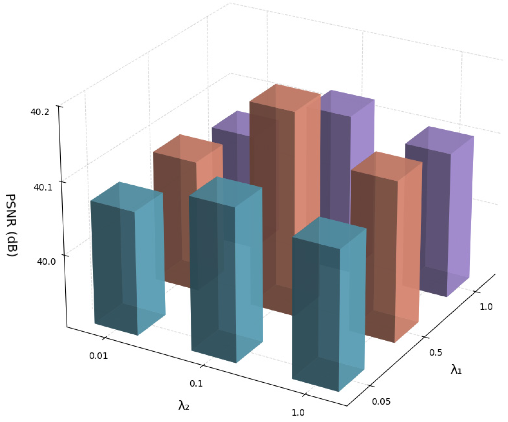
where ${\lambda }_1$ and ${\lambda }_2$ are the balancing parameters for the different loss terms, and the values of ${\lambda }_1$ and ${\lambda }_2$ are set to 0.5 and 0.1. This choice is informed by prior work [34] and is corroborated by our empirical analysis in Figure 10.

3. Results

3.1. Datasets

In this section, we evaluate the performance of the proposed method on three publicly available hyperspectral image datasets: CAVE [35], Harvard [36], and Chikusei [37].

CAVE dataset: This dataset comprises hyperspectral images of 32 distinct scenes, each accompanied by corresponding RGB images, capturing a wide range of real-world materials and objects. It consists of 31 spectral bands, spanning from 400 nm to 700 nm with 10 nm intervals, and a spatial resolution of 512 × 512 pixels.

Harvard dataset: The Harvard dataset contains hyperspectral images from 77 different scenes, including 50 indoor and outdoor environments and 27 indoor scenes under artificial or mixed lighting conditions.The dataset, it includes 31 spectral bands, covering the range from 420 nm to 720 nm with 10 nm intervals, and a spatial resolution of 1040 × 1392 pixels.

Chikusei dataset: Captured using the Hyperspec VNIR-C imaging sensor, this dataset includes hyperspectral imagery of agricultural and urban areas in Chikusei and Ibaraki, Japan. It features 128 spectral bands, spanning from 363 nm to 1018 nm, with a spatial resolution of 2517 × 2335 pixels and a ground sampling distance of 2.5 m.

The super-resolution (SR) performance was thoroughly assessed using a set of standard evaluation metrics: Peak Signal-to-Noise Ratio (PSNR), Structural Similarity Index (SSIM), Spectral Angle Mapper (SAM), Cross-Correlation (CC), Root Mean Square Error (RMSE), and the Relative Global Dimensionality Reduction Synthesis (ERGAS).

3.2. Implementation Rules

In this study, for both the CAVE and Harvard datasets, 80% of the samples were allocated for training, with the remaining 20% reserved for testing. To enhance the diversity of the training set, 24 image patches were randomly cropped from each image. The sample set was further augmented through three types of transformations: scale adjustments (applying scaling factors of 1, 0.75, and 0.5), rotational operations (rotating at 90°, 180°, and 270° angles), and horizontal/vertical flips. During preprocessing, bicubic downsampling was performed on images at scale factors of 2, 3, and 4 to generate low- resolution hyperspectral images with dimensions B × 32 × 32, where B denotes the number of spectral bands. For testing, to improve computational efficiency, only the top left 512 × 512 region of each test image was selected for evaluation. For the Chikusei dataset, due to the presence of invalid data in the edge regions, a central area of 2304 × 2048 × 128 pixels was first cropped for processing. Four non-overlapping images of size 512 × 512 × 128 were then extracted from the upper portion of the cropped region for testing, while the remaining area was used for training. When processing images at a scale factor of 4, image patches of 64 × 64 × 128 with a 32-pixel overlap were extracted; for a scale factor of 8, patches of 128 × 128 × 128 with a 128-pixel overlap were used. These patches were subsequently downsampled via bicubic interpolation to produce corresponding low resolution images at the specified scales.

In the proposed ESSTFormer network, for shallow spatial spectral feature extraction within the MSAM, dilated convolutions are employed with dilation rates set to 1, 3, and 5, respectively. Subsequently, spatial features are extracted using a 3 × 3 convolution kernel, while all other convolutions for channel expansion or shrinkage utilize 1 × 1 kernels. For deep spatial spectral feature extraction, the number of feature maps C in EETB and EATB is set to 240, and there are four consecutive EETB and EATB modules (see ablation study for details). Finally, a progressive upsampling strategy based on PixelShuffle is adopted to enlarge the spatial size of the input low-resolution hyperspectral image.

The network was trained using the Adam optimizer for 60 epochs, with a mini-batch size of 16 and an initial learning rate of 1 × 10⁻⁵. The model was implemented using the PyTorch 2.1.0, Meta Platforms, Inc., Menlo Park, CA, USA framework and trained on an NVIDIA RTX 4070 GPU (NVIDIA Corporation, Santa Clara, CA, USA).

3.3. Experimental Results and Analysis

3.3.1. Experimental Results on Chikusei

As shown in

Table 1. Quantitative comparison of different methods on the Chikusei dataset.

	d	PSNR	SAM	RMSE	CC
3DFCNN	4	38.6091	3.1174	0.0140	0.9355
MCNet	4	39.8950	2.4656	0.0112	0.9507
SSPSR	4	39.9955	2.3864	0.0119	0.9530
MSDFormer	4	40.0902	2.3981	0.0118	0.9539
Ours	4	40.1138	2.3635	0.0117	0.9542
3DFCNN	8	34.8375	4.8432	0.0215	0.8428
MCNet	8	35.5049	4.2785	0.0119	0.8661
SSPSR	8	35.1643	4.6911	0.0206	0.8560
MSDFormer	8	35.5914	4.1381	0.0197	0.8693
Ours	8	35.6314	4.0768	0.0195	0.8706

, we compared the proposed ESSTformer with several advanced methods on the Chikusei dataset and evaluated its performance under scale factors of ×4 and ×8 using four objective quantitative metrics. The comparative results demonstrate that ESSTformer outperforms other algorithms across all evaluation metrics. This superiority can be attributed to the fact that ESSTformer extracts local spatial spectral features via CNNs and further models long-range spatial spectral features separately by leveraging the heterogeneity of spatial and spectral features, thereby ultimately achieving an outstanding performance.

Specifically, although 3DFCNN [38] extracts spectral and spatial information through 3D convolutions, it fails to effectively capture critical spatial spectral features and suffers from a high computational complexity. MCNet [39] extracts the spatial spectral features of images by combining 2D and 3D convolutions, but still cannot capture global spatial spectral features due to the limitations of convolution kernels. SSPSR [40] adopts a grouping strategy, achieving a favorable performance in terms of spatial and spectral similarity. MSDFormer [41] also integrates CNN and Transformer architectures; despite its overall excellent performance, it is slightly inferior to ESSTformer in terms of PSNR and SAM metrics because it does not account for the heterogeneity between spectral and spatial features.

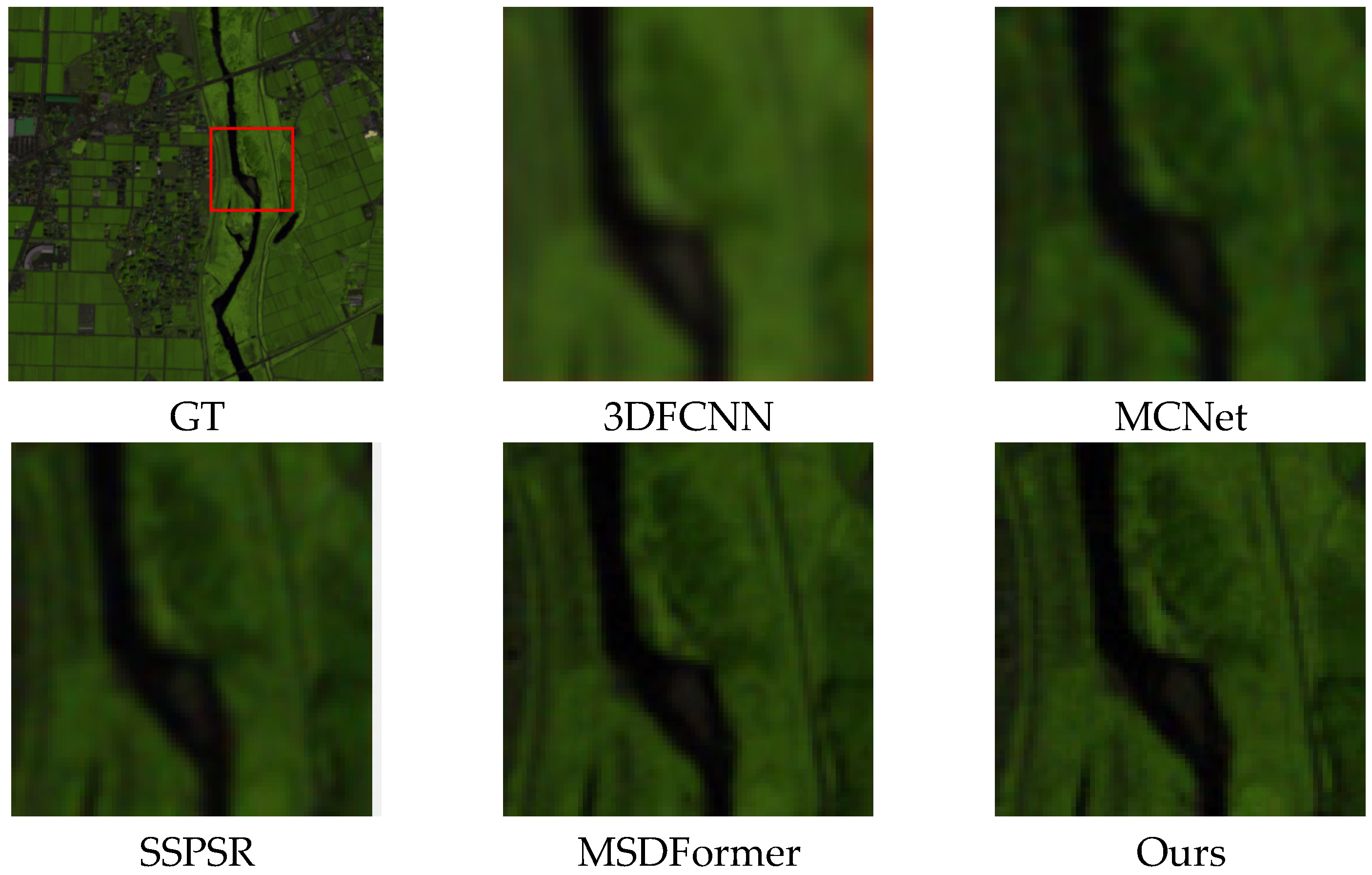
Qualitative results on the Chikusei dataset (Figure 6) demonstrate the advantage of our ESSTformer. CNN-based methods (3D-FCNN, MCNet, SSPSR) suffer from severe blurring due to limited receptive fields. A key differentiator is MSDFormer: while it uses a Spectral Transformer, it still relies on local convolutions for spatial detail recovery, restricting its global spatial modeling ability and leading to inconsistent spatial structure reconstruction (e.g., blurred field boundaries in Figure 6). Our ESSTformer addresses this with a decoupled dual-Transformer architecture: a dedicated Spatial Transformer explicitly captures long-range spatial contexts, working synergistically with the Spectral Transformer. This design enables ESSTformer to closely match the ground truth in both spatial sharpness (e.g., crisp river edges) and spectral consistency, outperforming MSDFormer and other methods.

3.3.2. Experimental Results on CAVE

As shown in

Table 2. Quantitative comparison of different methods on the CAVE dataset.

Metrics	d	3DFCNN	MCNet	SSPSR	MSDFormer	Ours
PSNR	2	44.154	45.092	-	45.204	45.484
SAM	2	2.405	2.301	-	2.333	2.359
SSIM	2	0.9786	0.9838	-	0.9856	0.9876
PSNR	3	40.219	42.031	-	42.345	42.589
SAM	3	2.930	2.809	-	2.672	2.548
SSIM	3	0.9653	0.9726	-	0.9754	0.9798
PSNR	4	37.326	39.207	38.366	39.6278	40.058
SAM	4	3.360	3.292	3.484	3.177	3.019
SSIM	4	0.9595	0.9654	0.9619	0.9672	0.9689

, we compared the proposed ESSTformer with several advanced methods on the CAVE dataset and evaluated its performance under scale factors of ×2, ×3, and ×4 using three objective quantitative metrics. The results demonstrate that ESSTformer achieves an excellent performance across all evaluation metrics, significantly outperforming other comparative methods. Due to its adoption of progressive upsampling, SSPSR [40] exhibits limited performance when the scale factor is small.

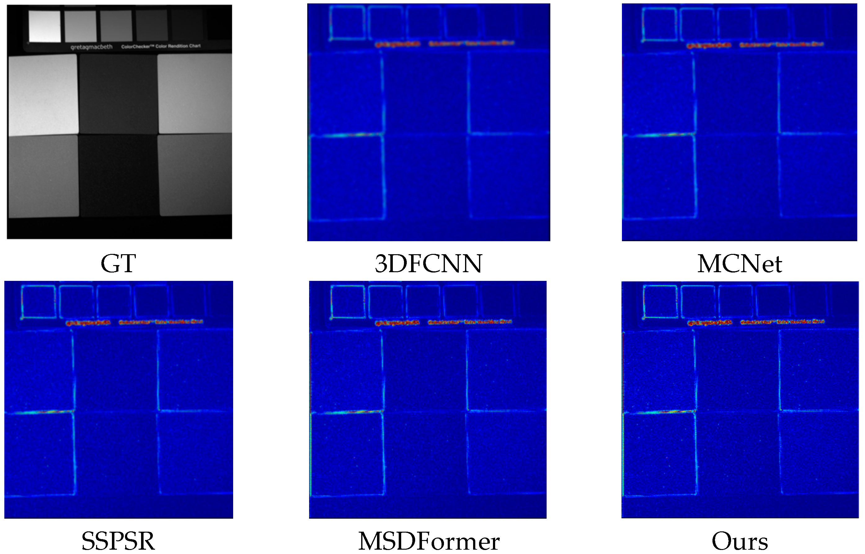
For evaluation, we randomly selected one test image from the CAVE dataset, displayed its spectral band, and analyzed the corresponding absolute error maps (Figure 7), with the GT as the reference. It is evident that 3DFCNN, MCNet, and SSPSR exhibit prominent error regions (brighter areas), indicating significant deviations in edge and texture reconstruction. MSDFormer reduces errors to some extent but still has noticeable residual errors. In contrast, ESSTFormer shows the darkest error map, meaning it has the smallest deviation from GT, directly demonstrating its superiority in spatial detail restoration and reconstruction fidelity. Such performance gain originates from our decoupled spatial spectral Transformer architecture and gated convolution module, which enable a more precise modeling of spatial textures in hyperspectral images.

3.3.3. Experimental Results on Harvard

As shown in

Table 3. Quantitative comparison of different methods on the Harvard dataset.

Metrics	d	3DFCNN	MCNet	SSPSR	MSDFormer	Ours
PSNR	2	45.264	46.213	-	46.642	46.985
SAM	2	1.794	1.703	-	1.613	1.644
SSIM	2	0.9808	0.9853	-	0.9865	0.9878
PSNR	3	42.385	43.681	-	43.912	44.151
SAM	3	2.930	1.987	-	1.903	1.817
SSIM	3	0.9580	0.9627	-	0.9653	0.9674
PSNR	4	39.037	40.544	40.474	40.635	40.866
SAM	4	2.185	2.108	2.201	2.014	2.001
SSIM	4	0.9219	0.9267	0.9241	0.9271	0.9297

, the ESSTformer proposed in this paper outperforms other methods on the Harvard dataset.

We selected a test image and displayed its spectral band for evaluation. As shown in Figure 8, the absolute error maps of multiple methods are presented to compare the spatial reconstruction performance. It can be seen from the figure that the reconstructed images exhibit clearer edges and more realistic visual information.

3.4. Ablation Experiments

(1)

Effectiveness of the multi-scale feature extraction module: In the MSAM, we employed dilated convolutions with three different dilation rates to extract multi-scale features of the image. To verify the effectiveness of multi-scale features, we replaced the dilated convolutions with standard convolutions to extract single-scale spatial spectral features and named this variant “Ours w/o DConv”. As indicated in

Table 4. Ablation studies on the Chikusei dataset.

Method	Params. (×${10}^6$)	FLOPs (×${10}^9$)	PSNR	SAM	RMSE	CC
Ours w/o DConv	15.8721	51.2243	40.0363	2.3889	0.0118	0.9533
Ours w/o EETB	14.4073	48.0436	39.9669	2.3979	0.0118	0.9526
Ours w/o SE	15.9265	52.1047	40.0809	2.3913	0.0117	0.9533
Ours w/o EATB	14.8562	49.6714	39.9973	2.3926	0.0118	0.9528
Ours w/o CMLP	15.7648	50.7129	39.8416	2.4196	0.0121	0.9512
Ours	16.0081	53.3816	40.1138	2.3635	0.0117	0.9542

, all performance metrics exhibit a noticeable degradation, further highlighting the critical role of multi-scale structures in super-resolution image reconstruction.

(2)

Effectiveness of the EETB module: In the proposed ESSTformer, we use the EETB module to capture the global spectral features of the image, thus enhancing the model’s representational capability. To evaluate the effectiveness of the EETB module, we replace it with a network made up of CNN modules. Specifically, we substitute the EETB module with the CA module, which is commonly used in SR, and name this modified model “Ours w/o EETB” as presented in Table 4. From the results, all metrics show a significant decrease.

(3)

Effectiveness of the SE Module: In the EETB, we introduce the SE module. It compresses squeeze and excitation in the features of each spectral channel, enabling the network to adaptively focus on more important spectral channels and thus enhance the spectral features. To verify the effectiveness of the SE module, we design a control network with the SE module removed, named “Ours w/o SE”. As can be seen from the results in Table 4, after removing the SE module, the network performance degrades, which further proves the crucial role of the SE module in improving network performance.

(4)

Effectiveness of the EATB module: In the proposed ESSTformer, considering the heterogeneity between spatial and spectral information in images, we process long-range spatial and spectral features separately. Specifically, we designed the EATB module to capture the global spatial features of images. To evaluate the effectiveness of the EATB module, we replaced it with a network composed of 2D convolution modules and named this variant “Ours w/o EATB” in Table 4. The experimental results demonstrate that, after removing the EATB module, all evaluation metrics exhibit a significant decline.

(5)

Effectiveness of the CMLP module: In conventional Transformers, the feed-forward network (FFN) module fails to fully capture the local spatial information in hyperspectral images. To address this limitation, we propose the CMLP module by integrating convolutional layers. To verify its effectiveness, we replaced the CMLP module with a standard MLP and labeled this variant “Ours w/o CMLP” in Table 4. The experimental results indicate that, after removing the CMLP module, the PSNR decreases significantly, which further confirms the critical role of the CMLP module in capturing the local spatial information of images.

(6)

To extract global spatial spectral information, we incorporate N Transformer modules into the network. The experimental results are presented in

Table 5. Number of Transformer modules.

Number	PSNR	SAM	RMSE	CC
N = 2	39.9110	2.4234	0.0121	0.9520
N = 4	40.1138	2.3635	0.0117	0.9542
N = 6	40.0528	2.3801	0.0118	0.9534
N = 8	39.9618	2.3891	0.0119	0.9401

. When fewer modules are used (N = 2), all quantitative metrics achieve the worst performance. When the number of Transformer modules increases to 4 (N = 4), metrics such as PSNR and SSIM improve significantly. However, with a further increase in the number of modules, the model complexity rises accordingly, leading to overfitting and subsequently a gradual decline in reconstruction performance.

(7)

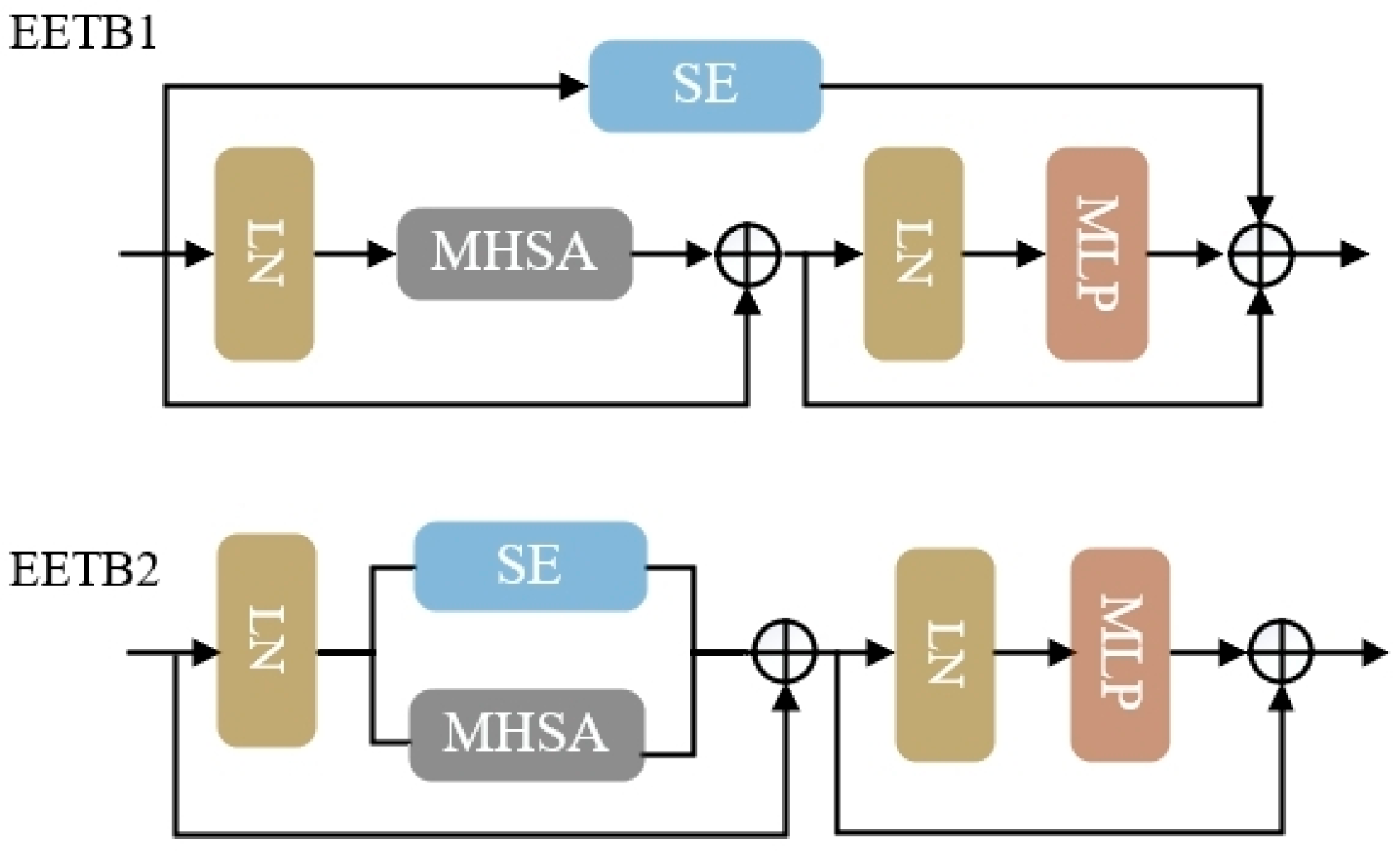
To determine the optimal position of the SE module within the EETB framework, we tested two variants, named EETB1 and EETB2, respectively. EETB1 places the SE module outside the EETB, while EETB2 embeds the SE module into the self-attention computation, as shown in Figure 9. The comparative experimental results, presented in

Table 6. Reconstruction results of SE at different positions.

Number	PSNR	SAM	RMSE	CC
EETB1	40.1013	2.3683	0.0117	0.9539
EETB2	40.1138	2.3635	0.0117	0.9542

, demonstrate that EETB2 achieves a superior reconstruction quality. The reason for this is that EETB2 can more effectively dynamically enhance the spectral information of images during feature computation, facilitating information interaction and fusion across different bands. Through this embedded approach, the model can more accurately capture the complex relationships between spatial and spectral information, thereby achieving better performance in super-resolution tasks.

(8)

Following prior work [34], we set the initial loss weights, ${\lambda }_1=0.5$ and ${\lambda }_2=0.1$. To confirm these hyperparameters for our task, we compared the PSNR values of different weight combinations on the Chikusei dataset. As shown in Figure 10, the PSNR indeed reaches its maximum when ${\lambda }_1=0.5$ and ${\lambda }_2=0.1$, which validates this setting and led us to its adoption.

4. Conclusions

In this paper, we propose a model named ESSTformer, which integrates the MSAM, EETB, and EATB modules to fully leverage the advantages of CNN structures and Transformer architectures in extracting local and global spatial spectral features. Specifically, the MSAM, composed of a multi-scale convolution module, a Residual Spatial Module, and a Residual Channel Attention Module, is designed to extract the shallow spatial spectral features of images. The EETB module extracts long-range spectral features based on the self-attention mechanism and is supplemented with a spectral enhancement module to help the network focus on important spectral features. Considering the heterogeneity of spatial and spectral information in images, the EATB module adopts a window-based attention mechanism to effectively capture global spatial features while reducing the computational complexity. Unlike traditional MLPs, the CMLP component in EATB pays more attention to the spatial neighborhood information of images, which is beneficial for the restoration of image details. Finally, the effectiveness of each module is verified through extensive ablation experiments. Both qualitative and quantitative experimental results demonstrate that the proposed method outperforms the existing methods on three hyperspectral image datasets, especially under different scale factors.