Abstract
Object detection technology plays a vital role in monitoring the growth status of aquaculture organisms and serves as a key enabler for the automated robotic capture of target species. Existing models for underwater biological detection often suffer from low accuracy and high model complexity. To address these limitations, we propose AOD-YOLO—an enhanced model based on YOLOv11s. The improvements are fourfold: First, the SPFE (Sobel and Pooling Feature Enhancement) module incorporates Sobel operators and pooling operations to effectively extract target edge information and global structural features, thereby strengthening feature representation. Second, the RGL (RepConv and Ghost Lightweight) module reduces redundancy in intermediate feature mappings of the convolutional neural network, decreasing parameter size and computational cost while further enhancing feature extraction capability through RepConv. Third, the MDCS (Multiple Dilated Convolution Sharing Module) module replaces the SPPF structure by integrating parameter-shared dilated convolutions, improving multi-scale target recognition. Finally, we upgrade the C2PSA module to C2PSA-M (Cascade Pyramid Spatial Attention—Mona) by integrating the Mona mechanism. This upgraded module introduces multi-cognitive filters to enhance visual signal processing and employs a distribution adaptation layer to optimize input information distribution. Experiments conducted on the URPC2020 and RUOD datasets demonstrate that AOD-YOLO achieves an accuracy of 86.6% on URPC2020, representing a 2.6% improvement over YOLOv11s, and 88.1% on RUOD, a 2.4% increase. Moreover, the model maintains relatively low complexity with only 8.73 M parameters and 21.4 GFLOPs computational cost. Experimental results show that our model achieves high accuracy for aquaculture targets while maintaining low complexity. This demonstrates its strong potential for reliable use in intelligent aquaculture monitoring systems.
1. Introduction
With the continuous exploitation and utilization of marine resources by humans, the effective detection of marine organisms has become a critical task [1,2]. Particularly in the field of aquaculture, object detection technology can not only be used to monitor the growth status of aquatic organisms in real time but also provide visual technical support for automated robotic fishing operations [3,4,5].
Early monitoring of aquaculture organisms primarily relied on visual observation or diver-based surveys, which were inefficient and challenging to implement on a large scale [6,7,8]. With technological advancements, cameras began to be used to capture underwater images for observation. In recent years, the rapid development of deep learning has enabled it to surpass traditional methods in both detection accuracy and speed, thereby facilitating automated monitoring. In the field of deep learning-based aquaculture object detection, existing methods can be broadly categorized into two types: two-stage detection algorithms and single-stage detection algorithms. While two-stage algorithms tend to be computationally slower, single-stage detectors such as YOLO [9] simplify the traditionally complex computations [10], resulting in significantly improved detection speed.
However, deep learning-based methods still face numerous challenges in underwater object detection. The underwater environment is complex and highly variable, while aquatic organisms exhibit diverse morphologies, vary significantly in size, and often exist in densely clustered groups [11,12,13,14]. These factors make it particularly difficult to accurately identify and distinguish individual biological targets in such complicated scenarios. Consequently, developing a high-precision underwater object detection algorithm is of great importance. Many researchers have improved the early algorithms, enhancing the model’s ability to recognize underwater targets.
Feature-level enhancements primarily focus on refining the internal representations within a given network architecture. These methods aim to boost the discriminative power of features, particularly for challenging underwater conditions. For instance, Cao et al. [15] and Liu et al. [16] built upon the Faster R-CNN framework by introducing dedicated RoI pooling and feature fusion mechanisms, respectively, to better capture object details and multi-scale contexts. Similarly, Feng et al. [17] developed the CEH-YOLO model, which incorporates modules to enhance feature extraction and color information processing. While these approaches effectively strengthen feature representation, they often operate within the constraints of the original backbone, potentially limiting their capacity for fundamental innovation and possibly leading to increased computational overhead.
In contrast, architecture-level redesigns involve more profound modifications to the network’s core components or connectivity to achieve a better balance between performance and efficiency. For example, Zhao et al. [18] proposed the YOLOv7-CHS algorithm by incorporating a novel CT module into the detection head to better capture contextual features. The work on YOLOv10 by Lu et al. [19] also falls into this category, as they designed a new MPFB module to augment the backbone’s feature extraction capability. Although these structural changes can be more efficient, they may not directly address the fundamental challenges of extracting robust features from degraded underwater images, such as blurry edges.
Meanwhile, the developers of YOLO models continue to release updated versions. However, these models still exhibit certain limitations in underwater target recognition.
YOLOv8 and YOLOv10, for instance, prioritize inference speed and architectural simplicity through their re-parameterization and lightweight design. However, this pursuit of efficiency often comes at the cost of feature richness. Their structures may lack dedicated components for enhancing fine-grained details and robust edge information, which are crucial for distinguishing blurred or camouflaged aquatic organisms. Consequently, they tend to underperform in scenarios requiring high discriminative power from degraded underwater imagery. Newer models like YOLOv12 incorporate advanced attention mechanisms to boost accuracy. Yet, these additions frequently introduce significant computational overhead and model complexity, moving them away from the lightweight deployment requirements essential for real-world aquaculture applications, such as deployment on embedded systems or autonomous underwater vehicles.
The models proposed by these researchers have achieved certain performance improvements. However, they still lack an optimal balance between accuracy and complexity. To address this limitation, this paper presents a novel model that maintains favorable complexity while achieving higher detection accuracy for aquaculture organisms in complex underwater environments.
2. Materials and Methods
The procedure of this research is as follows: dataset processing, algorithm design and improvement, and experimental validation. First, the selected dataset undergoes preprocessing and is randomly divided into training, validation, and test sets according to a predefined ratio. Subsequently, the YOLOv11s model is chosen as the baseline and is further enhanced and optimized based on the characteristics of the target objects. Finally, the accuracy of the proposed algorithm is experimentally validated and compared with other state-of-the-art methods to evaluate its performance.
2.1. Dataset Description
We conducted experiments on two public datasets: URPC2020 and RUOD. The URPC2020 dataset contains four types of target objects: holothurian, echinus, scallop, and starfish. After removing excessively blurred images, a total of 7000 images were selected. The dataset was randomly divided into training, validation, and test sets in a ratio of 6:2:2, resulting in 4200 images for training, 1400 for validation, and 1400 for testing. The RUOD dataset includes ten categories of objects to be detected: fish, jellyfish, holothurian, scallop, calamari, starfish, echinus, coral, diver and turtle. The original dataset provided 9800 training images and 4200 test images. Due to the lack of a dedicated validation set, the 9800 training images were further split into a new training set and a validation set at a ratio of 4:1, resulting in 7840 images for training and 1960 for validation.
2.2. AOD-YOLO Architecture
Based on YOLOv11s, this study introduces an improved model named AOD-YOLO, which consists of four main components: Input, Backbone, Neck, and Detect. The overall architecture of AOD-YOLO is illustrated in Figure 1.
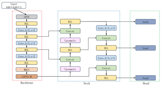
Figure 1.
The structure diagram of the AOD-YOLO.
2.2.1. Input
The Input module preprocesses the raw image. It resizes the image, scales pixel values, and converts the format from HWC to CHW. These steps standardize the data distribution, which enhances the model’s feature extraction and generalization performance.
2.2.2. Backbone
The Backbone is designed as a multi-layer convolutional network architecture. Shallow layers are more suitable for detecting small objects, while deeper layers excel at identifying larger targets, enabling effective recognition of objects across various scales. Simultaneously, the Backbone performs downsampling through convolutional and pooling operations, progressively reducing the spatial dimensions of feature maps and thus lowering computational complexity. The design of the Backbone critically influences the overall model performance, as it determines both the quality and efficiency of feature extraction.
2.2.3. Neck
The Neck module receives and further processes feature maps from the Backbone before passing them to the Head. It integrates multi-level features extracted by the Backbone and enhances them to improve the model’s capability in detecting objects of various sizes. By analyzing both shallow and deep features, the Neck constructs a multi-scale feature pyramid, effectively capturing small, medium, and large targets in the image.
2.2.4. Detect
The Detect module serves as the final output layer of the model. It decodes and makes predictions based on the multi-level features extracted by the Backbone and Neck, producing the final object detection results, which include bounding boxes, class labels, and confidence scores. For each grid cell in the feature maps, the Detect layer predicts multiple anchor boxes and outputs the corresponding coordinate offsets, class probabilities, and confidence scores for each anchor. The coordinate offsets are used to refine the initial position and size of the anchor boxes, enabling more accurate localization of target objects. The class probabilities indicate the likelihood of the target belonging to each category, while the confidence score reflects the probability that the anchor contains a valid object.
2.3. Improvement Methods
2.3.1. SPFE Module
In the task of detecting aquaculture objects, captured images often suffer from blurriness due to limitations such as underwater light scattering and poor illumination conditions. Traditional detection algorithms often underperform in extracting the appearance features of target objects. To address this, this paper proposes the SPFE module, which enables the complementarity and fusion of multi-level features, thereby capturing more detailed image characteristics. The structure of the SPFE module is illustrated in Figure 2.
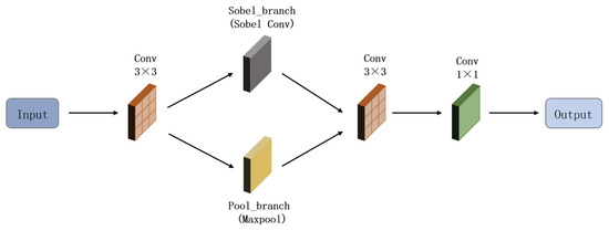
Figure 2.
The structure diagram of the SPFE Module.
The workflow of the proposed module is as follows: After receiving the input features, an initial convolution with a 3 × 3 kernel is applied for preliminary feature extraction and significant downsampling. The output splits into two branches: one uses a Sobel operator for edge detection, and the other applies pooling to capture global structure. The outputs of both branches are concatenated to form a combined feature map. This is followed by a second 3 × 3 convolution that fuses the multi-branch features and further reduces spatial resolution. A final 1 × 1 convolution is applied to adjust the channel dimension of the output features, producing the final result.
The SPFE module incorporates a dedicated Sobel convolution branch to extract edge features from the input. This design significantly enhances the model’s ability to capture blurred image contours and fine details in underwater environments. Compared to other classical operators such as Canny and Laplacian, the Sobel operator demonstrates distinct advantages in underwater detection scenarios. The Canny operator, for instance, requires threshold tuning that is highly sensitive to strong underwater noise, often resulting in fragmented or false edges. The Laplacian operator, while sensitive to edges, tends to amplify high-frequency noise in underwater images. In contrast, the Sobel operator offers greater robustness to noise, directional sensitivity, and computational efficiency, making it more suitable for detecting underwater objects. The structure of the Sobel convolution is illustrated in Figure 3.
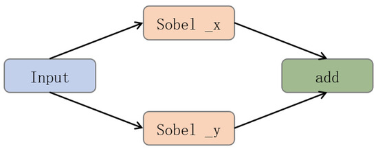
Figure 3.
The structure diagram of Sobel convolution.
Sobel edge detection is a classic gradient-based method for identifying edges by computing the gradient of the image intensity along both horizontal and vertical directions. It employs two sets of 3 × 3 kernels—one for horizontal edge detection and the other for vertical edge detection. Each kernel is convolved with the image to compute an approximation of the intensity gradients in its respective direction. The horizontal and vertical gradient responses are then combined to determine the edge strength at each pixel, allowing effective extraction of edge features from the image.
Let P represent the original image. The grayscale values of the images obtained after horizontal and vertical edge detection are denoted as and , respectively. Their calculations are defined as follows:
In the formula, * represents convolution operation, and P represents the original image.
The horizontal gradient value and the vertical gradient value at each pixel can be combined using the following formula to compute the gradient magnitude G:
Then the direction θ of the gradient can be calculated using the following formula:
Moreover, in addition to edge information, global contextual information is also crucial for understanding image content. Therefore, the SPFE module incorporates an additional pooling branch [20]. This branch plays a key role in capturing the global structural information of the image. It progressively reduces the spatial dimensions of the feature maps, thereby expanding the receptive field of subsequent layers and enabling the network to integrate local details into holistic representations. Additionally, by retaining the most salient local features, it enhances the model’s robustness to translation and minor deformations, while filtering out less relevant information. This results in more representative high-level features.
Finally, the SPFE module combines the edge features extracted by the Sobel branch with the global information captured by the pooling branch, achieving multi-dimensional integration. This fusion strategy preserves the sharpness of edge details while incorporating the comprehensive nature of spatial context, leading to more robust and discriminative feature representations. As a result, the model gains a more comprehensive ability to analyze image content accurately and provides stronger support for downstream tasks.
2.3.2. RGL Module
In response to the high demands for both accuracy and lightweight design in aquaculture object detection tasks, we conducted in-depth optimizations by removing the original C3K2 module and innovatively designing a lightweight and efficient module named RGL as its replacement. This modification not only reduces the number of parameters but also enhances feature extraction capability. The structure of the proposed RGL module is illustrated in Figure 4.
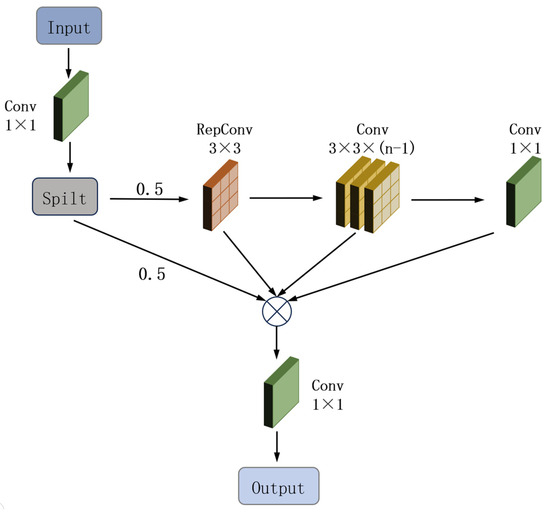
Figure 4.
The structure diagram of the RGL Module.
The workflow of the RGL module is structured as follows: First, a 1 × 1 convolution doubles the number of input channels, and the output is evenly split into two parts. The first part undergoes a 3 × 3 RepConv [21]. It is then processed through (n − 1) additional 3 × 3 convolutional layers to progressively extract features. By default, n is set to 1. Increasing n to 2 or 3 enhances the model’s representational capacity at the cost of a larger model size. Next, a 1 × 1 convolution [22] adjusts the channel dimension. All outputs from the branches are concatenated along the channel axis, followed by a final 1 × 1 convolution that fuses features from all paths to produce the output.
In the design of the RGL module, increasing the value of n incorporates more 3 × 3 convolutions into the model, leading to a significant rise in both parameter count and computational load. Since this model is intended for deployment in underwater detection equipment, it is crucial to maintain a lightweight architecture. Our experiments revealed that when using the RGL module with n = 1, the parameters reached 8.09 M and FLOPs amounted to 21.1 G. With n = 2, the parameters increased to 8.75 M and FLOPs to 23.5 G. The elevated value of n substantially heightened model complexity, which contradicts the requirements for underwater target detection. Therefore, we ultimately set n to 1.
To achieve both computational efficiency and high accuracy, traditional approaches often compress model size by reducing redundant features through techniques such as pruning and model compression. However, these methods often lead to a certain degree of accuracy loss during the compression process. To address the issue of high redundancy in intermediate feature maps of the YOLO11 model, this study draws inspiration from GhostNet [23] and introduces a lightweight feature generation mechanism for model compression. Specifically, the proposed method first employs 1 × 1 convolutions to reduce channel dimensionality, generating a compact set of intrinsic feature maps. These essential features then undergo a series of computationally efficient linear transformations to produce redundant features in a “ghost” manner. This process replaces the extensive dense convolution operations in traditional standard convolutions with extremely low-cost transformations, significantly reducing the model’s overall parameter count and computational complexity while maintaining the same total number of feature maps.
The 1 × 1 convolution is chosen for its ability to alter channel dimensionality without changing spatial resolution, greatly reducing computational and parametric overhead. For instance, when compressing the number of channels from 256 to 128, the number of parameters required is only one-ninth of that of a 3 × 3 convolution. Moreover, the 1 × 1 convolution facilitates cross-channel interaction and feature reorganization. By linearly combining features across channels, it effectively highlights critical information while reducing redundancy. In comparison, while 3 × 3 or larger convolutions can capture spatial local patterns, they incur higher computational costs. Larger kernels may also lead to loss of fine-grained details.
Furthermore, the original YOLO11 model employed the BottleNeck module [24], which consists of two convolutional layers aimed at feature extraction and computational reduction. However, due to its shallow structure with only two convolutional layers, this design prioritizes computational efficiency at the expense of limited non-linear representation capacity, potentially weakening feature extraction for small objects. To address this issue, the BottleNeck module was removed in our design. To compensate for the performance loss caused by its removal, we introduced RepConv in the gradient flow path.
We integrate a RepConv block into the main branch. During training, the RepConv block consists of a multi-branch structure: a 3 × 3 convolutional layer, a 1 × 1 convolutional layer, and an identity branch, each followed by a Batch Normalization (BN) layer. This diversity of paths enriches the feature space and improves gradient flow. During inference, this multi-branch structure is re-parameterized into a single 3 × 3 convolutional layer through a structural transformation, which combines the weights and BN statistics of all branches. This allows the model to retain the training-time performance benefits while maintaining the inference-time efficiency of a plain network. The structure of RepConv is illustrated in Figure 5.
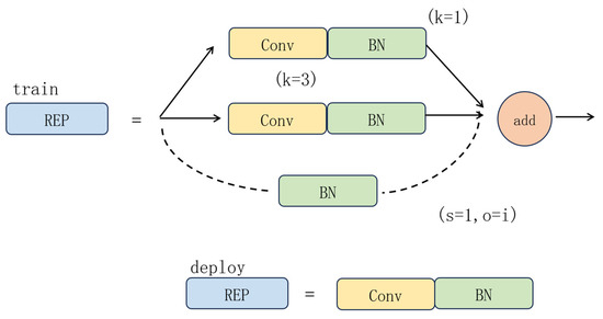
Figure 5.
The structure diagram of RepConv.
2.3.3. MDCS Module
In YOLO11, the SPPF module is employed for multi-scale feature fusion. Its design relies primarily on pooling operations, which reduce the spatial size of feature maps through downsampling [25] but inevitably discard some pixel-level information. However, in underwater environments, where target images often exhibit complex and detailed structures, the three consecutive pooling operations in SPPF can lead to excessive loss of fine-grained details, particularly impairing the detection of small biological objects. To address this limitation, we introduce the MDCS module, which incorporates dilated convolution with shared parameters. This design enhances the model’s capability to detect multi-scale targets while preserving more detailed information. The structure of the MDCS module is illustrated in Figure 6.
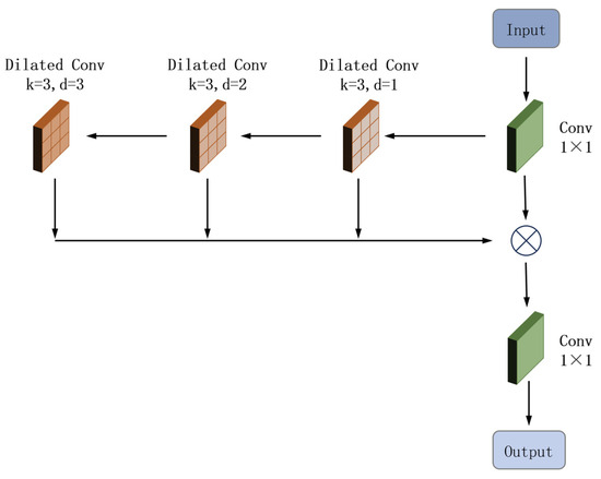
Figure 6.
The structure diagram of the MDCS Module.
The workflow of the MDCS module is as follows: First, the input feature map undergoes a 1 × 1 convolution for channel reduction. It is then processed by dilated convolutions with dilation rates of 1, 2, and 3, respectively, to extract multi-scale features. All resulting feature maps are concatenated along the channel dimension. The concatenated output is further fused through another 1 × 1 convolution, which integrates the multi-scale information and adjusts the channel dimensionality. Finally, the refined feature map is delivered as output.
By introducing intervals into a standard convolution kernel, dilated convolution effectively increases the receptive field. Given an input feature map of size with channels, and a desired output of channels using a kernel, the number of pixel layers of zero-padding added around the input feature map is .
The formula for the standard convolution computation A is:
A dilated convolution maintains the same computational cost as a standard convolution. In a dilated convolution, the kernel size is , and the dilation rate “” indicates that pixels are inserted between each element of the kernel. The receptive field refers to the spatial range of input information that a neuron can respond to. Its size is calculated using the following formula:
and represent the height and width of the input feature map, while and represent the height and width of the output. The following equations define the relationship between them:
As shown in the above formulas, when the dilation rate is 1, the dilated convolution is equivalent to a standard convolution. With a dilation rate of 2, each pixel in the convolutional kernel is separated by one pixel interval, resulting in a receptive field equivalent to that of a 5 × 5 standard convolution. Similarly, a dilation rate of 3 introduces two-pixel intervals between kernel elements, yielding a receptive field comparable to a 7 × 7 standard convolution. Convolutional kernels with smaller dilation rates specialize in capturing local features, while those with larger dilation rates can capture more global contextual information. Based on this principle, the MDCS module integrates three convolutional layers with different dilation rates. By fusing their information, it achieves a parameter-sharing mechanism that facilitates multi-scale feature capture. A schematic diagram illustrating dilated convolution is provided in Figure 7.
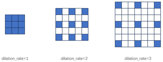
Figure 7.
Schematic diagram of Dilated Convolution.
The proposed design employs dilated convolutions with dilation rates of 1, 2, and 3. This combination enables a gradual expansion of the receptive field, avoiding abrupt jumps that could cause feature discontinuities, while also preventing the loss of local information associated with excessively large dilation rates. As a result, the module achieves a significant improvement in the detection capability for multi-scale objects.
2.3.4. C2PSA-M Module
The C2PSA module consists of two convolutional modules and two PSA [26] modules. In this work, we enhance the PSA module by integrating the Mona [27] module, recently proposed in CVPR 2025, which introduces multi-cognitive filters to strengthen the processing of visual signals. Additionally, a distribution adaptation layer is incorporated to optimize the input information. The overall structure of the C2PSA-M module is illustrated in Figure 8.
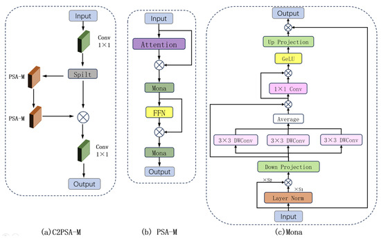
Figure 8.
The structure diagram of the C2PSA-M Module. (a) C2PSA-M Module; (b) PSA-M Module; (c) Mona Module.
The C2PSA-M module receives a feature map of size H × W × C as input. The integrated Mona module first normalizes the input through a distribution adaptation layer to stabilize the training process. Subsequently, the multi-cognitive filter branch applies three parallel depthwise convolutions with kernel sizes of 3 × 3, 5 × 5, and 7 × 7 to . Since depthwise convolutions are used, the channel dimension remains unchanged, producing three feature maps each of size . These three feature maps are then concatenated along the channel dimension to generate a fused feature map of size . A subsequent 1 × 1 convolutional layer projects the concatenated output back to the original dimension . Finally, a residual connection adds the result to the input . (In the description above, represents the height of the feature map, denotes the width of the feature map, indicates the number of input channels to the module, and represents the input tensor itself).
The Mona module is embedded within the PSA-M module, which itself is part of the larger C2PSA-M structure containing standard convolutional layers for deeper feature processing.
The workflow of the C2PSA-M Module is as follows: The input first passes through a 1 × 1 convolution to double the number of channels and is then split into two parts along the channel dimension: one part retains the original information, while the other part is enhanced through a module containing multiple PSA-M attention mechanisms. These two parts are then merged and passed through another 1 × 1 convolution to restore the channel count to its original state. This method effectively preserves the original features while introducing attention mechanisms to focus on more critical spatial information.
The core innovation of the Mona module lies in its incorporation of multi-cognitive filters, which utilize depth-wise convolutions with kernel sizes of 3 × 3, 5 × 5, and 7 × 7 to enhance the processing of visual signals. The Mona module uses three multi-scale convolutional layers with shared parameters. By fusing their information, it implements a parameter-sharing mechanism that facilitates multi-scale feature capture. Underwater images often present challenges like occlusion and significant scale variations. To address this, the multi-cognitive filtering mechanism in the Mona module enhances the model’s capability to extract and integrate features from blurred contours and multi-scale objects. This enables effective identification of diverse targets, thereby enriching feature representation and improving overall robustness.
Additionally, the Mona module optimizes input information. Given the substantial distributional differences between underwater image features and those in conventional images, a distribution adaptation layer (Scaled Layer Norm) is inserted at the front end of the adapter. This layer recalibrates and stabilizes the features extracted by the YOLO backbone, which may be affected by underwater distortions, adjusting their distribution to better suit the detection head. This adaptation not only stabilizes the model during fine-tuning or training but also enables faster convergence to the unique data distribution of underwater datasets, thereby improving training efficiency.
3. Experiments
3.1. Experimental Environment and Related Parameters
In order to ensure fairness in the experiment, the experimental environment and relevant parameters were kept consistent. The specific experimental configuration is shown in Table 1.

Table 1.
Experimental configuration.
3.2. Evaluation Metrics
Following the training phase, we utilized the val.py script to validate the model’s performance. This script outputs a comprehensive set of detection metrics upon completion. We selected the following metrics to evaluate the performance of our improved model.
(1) mAP (Mean Average Precision):
Object detection tasks often require identifying multiple objects. The mAP metric reflects the average precision of the algorithm across all target categories, representing its overall detection accuracy. Here, Average Precision (AP) denotes the average precision value for a single category under varying recall rates.
mAP50: The mean average precision calculated when the Intersection over Union (IoU) between predicted and ground-truth bounding boxes is greater than or equal to 0.5.
mAP50:95: This metric is calculated by averaging performance across multiple stringent IoU thresholds ranging from 0.5 to 0.95. Here, IoU measures the degree of overlap between predicted bounding boxes and ground truth boxes.
(2) P (Precision):
This metric indicates the proportion of correctly identified objects among all detections made by the algorithm. Precision reflects the model’s ability to accurately localize objects and predict their categories. It is defined by the following formula:
In the formula, represents the number of positive samples predicted by the model, which is actually the number of positive samples. represents the number of negative class samples that the model incorrectly predicts as positive class samples.
(3) R (Recall): refers to the proportion of all positive samples correctly predicted by the model as positive samples, reflecting the comprehensiveness and coverage of the model for object detection. The calculation formula is as follows.
In the formula, FN represents the number of actual targets that were not detected by the model
(4) Params (Parameters): It reflects the complexity of the model, and the larger its value, the more complex the model. More complex models usually have better ability to detect targets.
(5) GFLOPs: This parameter measures the computational complexity of the model by counting the number of floating-point operations required to complete one forward propagation.
(6) FPS: It represents the number of images the model can process per second, with a higher value indicating greater processing capability. Generally, when the FPS exceeds 30, the processing capacity is considered strong.
3.3. Performance Comparison and Analysis of Results
To validate the improvements achieved by AOD-YOLO, I conducted comparative experiments under identical conditions using both the YOLOv11s baseline model and our proposed AOD-YOLO model on the URPC2020 and RUOD datasets. All conclusions were derived from the average of three experimental trials, with both mAP50 and mAP50:95 reported as mean ± standard deviation. Table 2 shows the comparison of improved models on the URPC2020 dataset, while Table 3 shows the comparison of improved models on the RUOD dataset.
Table 2.
Comparison of Improved Models on URPC2020 Dataset.
Table 3.
Comparison of Improved Models on RUOD Dataset.
As shown in Table 2 and Table 3, the proposed AOD-YOLO model consistently outperforms the YOLOv11s baseline on both datasets. Specifically, on the URPC2020 dataset, AOD-YOLO achieves an mAP50 of 86.6%, a 2.6% improvement over YOLOv11s. Similarly, on the RUOD dataset, our model attains an mAP50 of 88.1%, which is 2.4% higher than the baseline. Furthermore, significant improvements are observed in mAP50:95, precision, and recall metrics, accompanied by a reduction of 0.68 million parameters. These results demonstrate the effectiveness of the proposed improvements.
To demonstrate the detection performance of the AOD-YOLO model for each target category, Table 4 and Table 5 present the recognition accuracy of the model for various target types on the URPC2020 and RUOD datasets, respectively. The data in the tables indicate that the AOD-YOLO model achieves superior detection accuracy compared to YOLOv11s and exhibits robust detection capability across all target categories.
Table 4.
The accuracy of the model for target recognition in URPC 2020 dataset (mAP50).
Table 5.
The accuracy of the model for target recognition in RUOD dataset (mAP50).
3.4. Ablation Experiments
To evaluate the contribution of each module in the AOD-YOLO model, this study employs YOLOv11s as the baseline and incrementally incorporates different components. All experiments were conducted under identical environmental conditions and parameter settings on both the URPC2020 and RUOD datasets. A “√” indicates the usage of the corresponding module. The ablation results on the URPC2020 dataset are presented in Table 6, while those on the RUOD dataset are shown in Table 7.
Table 6.
Experimental results of ablation using URPC2020 dataset.
Table 7.
Experimental results of ablation using RUOD dataset.
The ablation study results demonstrate that each improvement proposed in this paper contributes significantly to detection performance. The AOD-YOLO model achieves a detection accuracy of 86.6% on the URPC2020 dataset, which is 2.6% higher than that of YOLOv11s, and an accuracy of 88.1% on the RUOD dataset, representing a 2.4% improvement over YOLOv11s. Meanwhile, on both datasets, the AOD-YOLO model demonstrates improvements in both precision and recall. This indicates that AOD-YOLO successfully reduces false positives while missing fewer true targets, effectively breaking the typical trade-off between these two metrics. Finally, AOD-YOLO has only 8.73 M parameters, which is 0.68 M fewer than YOLOv11s, while GFLOPs remains nearly identical. This validates the effectiveness of our RGL module in designing a more efficient and powerful architecture.
Figure 9 presents a comparison of detection accuracy between YOLOv11s and AOD-YOLO on the URPC2020 dataset, Figure 10 shows the corresponding comparison on the RUOD dataset. As shown in Figure 9 and Figure 10, the AOD-YOLO model achieves higher precision at the same recall rates across different datasets, with its average precision curve positioned closer to the top-right corner. This proves that the model has better detection performance.

Figure 9.
Comparison of Detection Accuracy between YOLOv11s and AOD-YOLO Models on URPC2020 Dataset. (a) YOLOv11s; (b) AOD-YOLO.
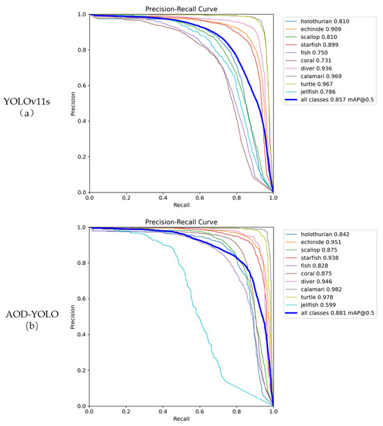
Figure 10.
Comparison of detection accuracy between YOLOv11s and AOD-YOLO models on the RUOD dataset. (a) YOLOv11s; (b) AOD-YOLO.
3.5. Comparison Experiments
3.5.1. Comparative Experiments of Overall Models
To evaluate the performance of the AOD-YOLO model, this study conducted comparative experiments under identical experimental environments and parameter settings, comparing it against state-of-the-art object detection algorithms. Table 8 presents a comparative analysis of detection results between AOD-YOLO and other advanced models on the URPC2020 dataset, while Table 9 provides the corresponding comparison on the RUOD dataset.
Table 8.
Comparative experimental results using URPC2020 dataset.
Table 9.
Comparative experimental results using RUOD dataset.
3.5.2. Comparative Experiments on the C3K2 Module Improvement
In this study, the original C3K2 module was removed and replaced with the proposed RGL module. Since numerous classical improved versions of the C3K2 module already exist, a comparative experiment was conducted under consistent experimental conditions and parameters to systematically evaluate the performance advantages of the RGL module. The results of the comparative experiments on the C3K2 module improvements are presented in Table 10.
Table 10.
Comparison experiment results of C3K2 module improvement.
Experimental results demonstrate that the RGL module achieves the highest detection accuracy on both the URPC2020 and RUOD datasets. Compared to the original C3K2 module in YOLOv11s, it improves accuracy by 0.8% and 1.0%, respectively. Furthermore, the proposed module exhibits superior detection performance and stronger generalization capability when compared to other classical modules.
3.6. Image Detection Comparison Experiments
To visually demonstrate the detection accuracy and the underlying strengths of the proposed model, comparative experiments were conducted on various challenging underwater images. As illustrated in Figure 11, four representative image groups were selected, each displaying the original image alongside detection results from YOLOv8s, YOLOv11s, and the proposed AOD-YOLO model. The following analysis provides a thorough commentary on these results.
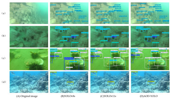
Figure 11.
Comparison of detection results of different algorithms. (A) Original image; (B) YOLOv8s model; (C) YOLOv11s model; (D) AOD-YOLO model.
(a) Scene with numerous small targets. While all three algorithms successfully detect all sea urchins present, the proposed AOD-YOLO model demonstrates consistently and significantly higher confidence scores across all detections. This performance can be attributed to our proposed modules: The MDCS module enhances multi-scale feature extraction, which is crucial for small objects, by preserving fine-grained details often lost in the SPPF structure of the baseline models. Simultaneously, the C2PSA-M module, with its multi-cognitive filters, allows the model to better focus on the distinctive features of small, clustered targets, leading to more confident and accurate predictions.
(b) Scene with a blurry image and a fragmented object. In this challenging case, a partially visible sea urchin on the far right is incorrectly identified as two separate objects by both YOLOv8s and YOLOv11s, while our algorithm accurately recognizes it as a single instance. Furthermore, a stone in the lower left corner is misidentified as a starfish by the comparison models, whereas our method correctly rejects this false positive. This robustness is primarily due to the SPFE module. The Sobel branch within SPFE strengthens the model’s ability to extract robust edge information even from blurry images, helping to delineate the true contour of the fragmented sea urchin. The pooling branch captures global context, aiding in distinguishing non-biological structures from actual marine organisms.
(c) Scene with mutual occlusion and a false positive. Here, YOLOv8s generates a false positive detection of a scallop in the lower left area, while both YOLOv11s and our algorithm correctly reject it. In areas with significant inter-species occlusion, the proposed method maintains the highest confidence levels for correctly identified objects. The enhanced performance in occluded scenarios is achieved through the synergistic effect of the C2PSA-M and SPFE modules. The C2PSA-M module’s attention mechanism helps the model focus on the most discriminative parts of a partially visible target, while the SPFE module’s edge-enhanced features provide crucial contour information that persists even when targets overlap.
(d) Scene with a camouflaged target. The original image contains a calamari that exhibits strong similarity to the background environment. Although all algorithms successfully detect the target, the proposed AOD-YOLO model achieves a substantially higher detection confidence. This superior performance against camouflage is a direct result of the feature representation enhancements. The RGL module, with its efficient feature generation and RepConv, reduces feature redundancy and enhances the discriminative power of the extracted features. This, combined with the multi-scale perception of the MDCS module, allows our model to better capture the subtle features that distinguish the camouflaged calamari from its background, resulting in a more confident prediction.
3.7. Comparison of Heat Maps
To intuitively demonstrate the feature extraction capability and the model’s focus regions of the proposed model, class activation mapping was employed to generate heatmaps, which were visualized using the built-in visualization component of the YOLOv11 framework. It is critical to clarify that these heatmaps represent the model’s activation intensity, or “attention”, toward potential targets, not physical temperature. In these visualizations, the color gradient indicates confidence levels, with red indicating high-confidence regions and blue representing low-confidence areas. A greater presence of red regions indicates superior feature extraction performance and that the model is focusing on the correct areas of the image. As shown in Figure 12, four image groups are presented, each containing the original image alongside heatmaps produced by YOLOv8s, YOLOv11s, and the proposed AOD-YOLO model.
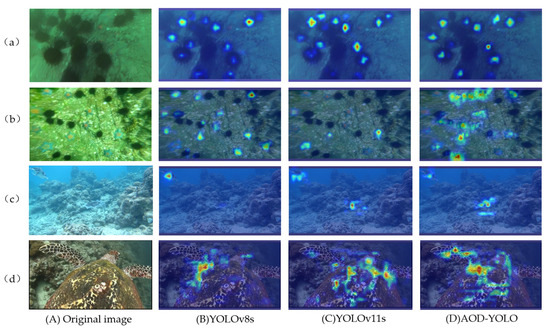
Figure 12.
Comparison of heat maps between AOD-YOLO model and other models. (A) Original image; (B) YOLOv8s model; (C) YOLOv11s model; (D) AOD-YOLO model.
The comparative analysis of heatmaps indicates that, compared to YOLOv8s and YOLOv11s, the AOD-YOLO model exhibits the most extensive activated regions with the most prominent red areas, demonstrating its enhanced capability in recognizing characteristic features of target objects. The YOLOv8s model fails to detect sea cucumbers, scallops, and squids in certain cases, while YOLOv11s identifies these species but with suboptimal accuracy. In contrast, the proposed AOD-YOLO model effectively detects these marine organisms, showing distinct red activations, and also achieves superior recognition performance for other targets.
4. Failure Cases and Limitations
While the AOD-YOLO model has demonstrated superior overall performance across multiple datasets, our detailed post hoc analysis reveals certain limitations in challenging scenarios.
First, the model continues to demonstrate insufficient sensitivity to targets with high background similarity or camouflage coloration. As shown in Figure 13, the visual characteristics of the target objects closely resemble those of the background environment. In such scenarios, despite the enhanced edge extraction capability of the SPFE module, the extremely low contrast between the target and background makes it challenging for the model to extract sufficient discriminative features, resulting in relatively low confidence scores.
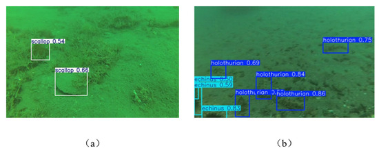
Figure 13.
Detection results for targets with high background similarity. (a) Scallop images with similar background; (b) Images of echini and holothurians with similar background.
Second, the model’s performance heavily depends on the quality and representativeness of training data. Although the current model was trained on URPC2020 and RUOD datasets—which represent typical underwater environments in terms of species diversity, shooting angles, and lighting conditions—they fall short of capturing the full complexity of real-world scenarios. Furthermore, under extreme underwater conditions such as highly turbid waters, overexposure caused by strong artificial lighting, or extremely low-light environments, the sharp degradation in image quality leads to significant performance decline for all vision-based detection models, including AOD-YOLO.
In summary, future research will focus on creating more robust feature representations for low-contrast targets. We plan to implement advanced data augmentation techniques designed specifically for underwater conditions. These methods will simulate challenges like turbidity and color distortion to enhance model performance in extreme visual environments. Additionally, we will expand our training dataset with more diverse and challenging underwater samples. The model architecture will also be further optimized to improve its overall capability.
5. Conclusions
To address the issues of low detection accuracy and high model complexity in existing algorithms for underwater organism recognition, this paper proposes the AOD-YOLO model. Based on YOLOv11s, the model enhances performance through four key improvements. First, the SPFE module incorporates Sobel operators and pooling operations to extract target edge information and global structural features, thereby improving feature extraction capability. Next, the RGL module reduces redundancy in the network, decreasing both parameter count and computational complexity, while further enhancing feature representation through RepConv. The MDCS module then replaces the SPPF structure, integrating parameter-shared dilated convolutions to boost multi-scale target detection. Finally, the C2PSA module is upgraded to C2PSA-M using the Mona mechanism, which introduces multi-cognitive filters for improved visual signal processing and employs a distribution adaptation layer to optimize input information. Systematic experiments demonstrate that the proposed model achieves excellent detection performance for various aquaculture species, accurately identifying target organisms with higher precision compared to other state-of-the-art algorithms. Evaluations on multiple datasets confirm its strong generalization capability. With a parameter count of 8.73 M and a computational cost of 21.4 GFLOPs, the model maintains relatively low complexity. Owing to its outstanding performance, AOD-YOLO can be deployed on detection devices to support the digital transformation of the aquaculture industry.
Author Contributions
Conceptualization, Y.F.; methodology, C.L. and W.S.; software, Y.F.; validation, Y.F. and D.C.; formal analysis, J.Z.; investigation, C.L.; resources, Y.F.; writing—original draft preparation, Y.F.; writing—review and editing, Y.F. and J.Z.; visualization, Y.F. and W.S.; supervision, Y.F. and D.C.; project administration, C.L. and J.Z. All authors have read and agreed to the published version of the manuscript.
Funding
This research received no external funding.
Institutional Review Board Statement
Not applicable.
Informed Consent Statement
Not applicable.
Data Availability Statement
The original contributions presented in this study are included in the article. Further inquiries can be directed to the corresponding author.
Acknowledgments
We would like to express our gratitude to the teachers and students of Shanghai Ocean University for their assistance and technical support in this research.
Conflicts of Interest
The author declares that there is no conflict of interest.
References
- Liu, L.; Li, P. Plant intelligence-based PILLO underwater target detection algorithm. Eng. Appl. Artif. Intell. 2023, 126, 106818. [Google Scholar] [CrossRef]
- Xu, S.; Zhang, M.; Song, W.; Mei, H.; He, Q.; Liotta, A. A systematic review and analysis of deep learning-based underwater object detection. Neurocomputing 2023, 527, 204–232. [Google Scholar] [CrossRef]
- Li, X.; Zhao, Y.; Su, H.; Wang, Y.; Chen, G. Efficient underwater object detection based on feature enhancement and attention detection head. Sci. Rep. 2025, 15, 5973. [Google Scholar] [CrossRef] [PubMed]
- Li, T.; Gang, Y.; Li, S.; Shang, Y. A small underwater object detection model with enhanced feature extraction and fusion. Sci. Rep. 2025, 15, 2396. [Google Scholar] [CrossRef] [PubMed]
- Kumar, A.; Berar, G.; Sharma, M.; Sakshi; Noonia, A.; Verma, G. Underwater image enhancement using hybrid transformers and evolutionary particle swarm optimization. Sci. Rep. 2025, 15, 29575. [Google Scholar] [CrossRef] [PubMed]
- Diamant, R.; Kipnis, D.; Bigal, E.; Scheinin, A.; Tchernov, D.; Pinchasi, A. An Active Acoustic Track-Before-Detect Approach for Finding Underwater Mobile Targets. IEEE J. Sel. Top. Signal Process. 2019, 13, 104–119. [Google Scholar] [CrossRef]
- Wang, M.; Zhang, K.; Wei, H.; Chen, W.; Zhao, T. Underwater image quality optimization: Researches, challenges, and future trends. Image Vis. Comput. 2024, 146, 104995. [Google Scholar] [CrossRef]
- Ding, J.; Hu, J.; Lin, J.; Zhang, X. Lightweight enhanced YOLOv8n underwater object detection network for low light environments. Sci. Rep. 2024, 14, 27922. [Google Scholar] [CrossRef]
- Redmon, J.; Divvala, S.; Girshick, R.; Farhadi, A. You only look once: Unified, real-time object detection. In Proceedings of the IEEE Conference on Computer Vision and Pattern Recognition, Las Vegas, NV, USA, 26 June–1 July 2016; pp. 779–788. [Google Scholar]
- Liu, W.; Anguelov, D.; Erhan, D.; Szegedy, C.; Reed, S.; Fu, C.Y.; Berg, A.C. Ssd: Single shot multibox detector. In Proceedings of the Computer Vision–ECCV 2016: 14th European Conference, Amsterdam, The Netherlands, 11–14 October 2016; pp. 21–37. [Google Scholar]
- Luo, Y.; Eljamal, O. SPyramidLightNet: A Lightweight Shared Pyramid Network for Efficient Underwater Debris Detection. Appl. Sci. 2025, 15, 9404. [Google Scholar] [CrossRef]
- Xu, W.; Fang, H.; Yu, S.; Yang, S.; Yang, H.; Xie, Y.; Dai, Y. RSNC-YOLO: A Deep-Learning-Based Method for Automatic Fine-Grained Tuna Recognition in Complex Environments. Appl. Sci. 2024, 14, 10732. [Google Scholar] [CrossRef]
- Guo, A.; Sun, K.; Zhang, Z. A lightweight YOLOv8 integrating FasterNet for real-time underwater object detection. J. Real Time Image Process. 2024, 21, 49. [Google Scholar] [CrossRef]
- Qu, S.; Cui, C.; Duan, J.; Lu, Y.; Pang, Z. Underwater small target detection under YOLOv8-LA model. Sci. Rep. 2024, 14, 16108. [Google Scholar] [CrossRef]
- Cao, C.; Wang, B.; Zhang, W.; Zeng, X.; Yan, X.; Feng, Z.; Liu, Y.; Wu, Z. An Improved Faster R-CNN for Small Object Detection. IEEE Access 2019, 7, 106838–106846. [Google Scholar] [CrossRef]
- Liu, Y.; Wang, S. A quantitative detection algorithm based on improved faster R-CNN for marine benthos. Ecol. Inform. 2021, 61, 101228. [Google Scholar] [CrossRef]
- Feng, J.; Jin, T. CEH-YOLO: A composite enhanced YOLO-based model for underwater object detection. Ecol. Inform. 2024, 82, 102758. [Google Scholar] [CrossRef]
- Zhao, L.; Yun, Q.; Yuan, F.; Ren, X.; Jin, J.; Zhu, X. YOLOv7-CHS: An Emerging Model for Underwater Object Detection. J. Mar. Sci. Eng. 2023, 11, 1949. [Google Scholar] [CrossRef]
- Lu, Z.; Liao, L.; Xie, X.; Yuan, H. SCoralDet: Efficient real-time underwater soft coral detection with YOLO. Ecol. Inform. 2025, 85, 102937. [Google Scholar] [CrossRef]
- Gholamalinezhad, H.; Khosravi, H. Pooling methods in deep neural networks, a review. arXiv 2020, arXiv:2009.07485. [Google Scholar] [CrossRef]
- Ding, X.; Zhang, X.; Ma, N.; Han, J.; Ding, G.; Sun, J. Repvgg: Making vgg-style convnets great again. In Proceedings of the IEEE/CVF Conference on Computer Vision and Pattern Recognition, Nashville, TN, USA, 20–25 June 2021; pp. 13733–13742. [Google Scholar]
- Woo, S.; Park, J.; Lee, J.-Y.; Kweon, I.S. Cbam: Convolutional block attention module. In Proceedings of the European Conference on Computer Vision (ECCV), Munich, Germany, 8–14 September 2018; pp. 3–19. [Google Scholar]
- Han, K.; Wang, Y.; Tian, Q.; Guo, J.; Xu, C.; Xu, C. Ghostnet: More features from cheap operations. In Proceedings of the IEEE/CVF Conference on Computer Vision and Pattern Recognition, Seattle, WA, USA, 13–19 June 2020; pp. 1580–1589. [Google Scholar]
- Koh, P.W.; Nguyen, T.; Tang, Y.S.; Mussmann, S.; Pierson, E.; Kim, B.; Liang, P. Concept bottleneck models. In Proceedings of the International Conference on Machine Learning, Online, 13–18 July 2020; pp. 5338–5348. [Google Scholar]
- Zhou, D.X. Theory of deep convolutional neural networks: Downsampling. Neural Netw. 2020, 124, 319–327. [Google Scholar] [CrossRef]
- Liu, H.; Liu, F.; Fan, X.; Huang, D. Polarized self-attention: Towards high-quality pixel-wise regression. arXiv 2021, arXiv:2107.00782. [Google Scholar]
- Yin, D.; Hu, L.; Li, B.; Zhang, Y.; Yang, X. 5%> 100%: Breaking performance shackles of full fine-tuning on visual recognition tasks. In Proceedings of the Computer Vision and Pattern Recognition Conference, Nashville, TN, USA, 11–15 June 2025; pp. 20071–20081. [Google Scholar]
- Tian, Y.; Ye, Q.; Doermann, D. Yolov12: Attention-centric real-time object detectors. arXiv 2025, arXiv:2502.12524. [Google Scholar]
- Xin, S.; Ge, H.; Yuan, H.; Yang, Y.; Yao, Y. Improved lightweight underwater target detection algorithm for YOLOv7. J. Comput. Eng. Appl. 2024, 60, 88–99. [Google Scholar]
- Yuan, H.; Li, C. Research on FDC-YOLO v8 Underwater Biological Object Detection Method Improved by Deformable Convolution. Trans. Chin. Soc. Agric. Mach. 2024, 55, 140–146. [Google Scholar]
- Jiang, Z.; Hu, L. Marine life identification method based on improved RT-DETR. Electron. Meas. Technol. 2024, 47, 155–163. [Google Scholar]
Disclaimer/Publisher’s Note: The statements, opinions and data contained in all publications are solely those of the individual author(s) and contributor(s) and not of MDPI and/or the editor(s). MDPI and/or the editor(s) disclaim responsibility for any injury to people or property resulting from any ideas, methods, instructions or products referred to in the content. |
© 2025 by the authors. Licensee MDPI, Basel, Switzerland. This article is an open access article distributed under the terms and conditions of the Creative Commons Attribution (CC BY) license (https://creativecommons.org/licenses/by/4.0/).