Featured Application
The proposed method enables the rapid determination of aerodynamic resistance in ventilation sidings of underground mine workings using laser scanning.
Abstract
Accurate assessment of aerodynamic resistance in mine ventilation networks is essential for ensuring operational safety and energy efficiency, yet traditional measurement approaches remain time-consuming and prone to uncertainty. This study presents a novel methodology for constructing digital ventilation models of underground mine workings using markerless LiDAR scanning combined with automated data processing. The proposed procedure includes segmentation of point clouds into sections, calculation of geometric parameters, and direct determination of resistance coefficients, which are subsequently exported to VentSim software. The approach was validated through a case study conducted in a Polish coal mine, where a 369 m ventilation siding was scanned and analyzed. The comparison between numerical simulations and in situ measurements demonstrated strong agreement, with differences not exceeding ±5% for airflow velocity, pressure drop, and total flow rate, while larger deviations were observed for cross-sectional area (+5.1%). The method is limited by potential inaccuracies in determining excavation geometry, which can lead to errors in calculating resistance coefficients, particularly at excavation intersections and at the beginning and end of scanning sections. Point cloud analysis, determination of resistance coefficients for individual sections (segments), spatial transformation, and point cloud reduction, along with integration with VentSim, are based on Python scripts. Calculation results can be easily exported to other computational programs. The proposed approach enables integration with various sensors and allows for assigning this value directly to a given section (segment of the excavation). The method can support the construction of digital twins for mines or underground tunnels. The implementation codes of the developed algorithms have also been made available for educational and scientific purposes under the Modified GNU General Public License v3 (GPLv3).
1. Introduction
Accurate knowledge of the current airflow and the physicochemical parameters of the air in mine workings is fundamental for the safe execution of operations in underground mining facilities, especially under conditions of natural and ventilation hazards (fire, methane, climate, rock bursts) [1]. Underground ventilation networks of deep mines usually have a complex structure (several hundred ventilation sidings, total workings length exceeding 100 km, and a serial-parallel arrangement of sidings with the occurrence of diagonal airflows). It often happens that the ventilation networks of neighboring mining facilities interact with each other, for example, through connections in post-mining goafs. Inaccurate knowledge of airflow distribution, aerodynamic potential, temperature, humidity, or the composition of the mine atmosphere affects both the safety level of mining crews and production.
Research on mine ventilation simulation has progressively advanced from traditional network models to more sophisticated computational and three-dimensional approaches. A central methodological development is the use of computational fluid dynamics (CFD) for airflow, gas, and dust simulations in underground environments. CFD methods typically involve solving the Navier–Stokes equations supplemented with turbulence models. A review carried out by Yi et al. [2] showed that CFD is a useful tool for studying airflow and gas or dust dispersion in underground mines. Authors highlighted discrepancies between CFD simulations and experimental results remain, mainly due to wall roughness, challenges in accurately modeling mining environments, grid quality issues, and turbulence model selection. Nevertheless, accounting for rough surfaces and using accurate airflow data can improve CFD accuracy and its effectiveness in mine ventilation analysis. Kanam and Ahmed [3] conducted a comprehensive review of previous studies concerning the design and optimization of ventilation systems. Their analysis indicated that the most effective and accurate methods for optimizing ventilation in underground mines include the iterative Hardy-Cross method, adjustments in airflow quantity and direction, finite-step iteration, and the categorization of nodes. Ventsim software is widely employed due to its reliability and flexibility in calculating parameters such as flow rate, shaft depth, fan placement, and other specific characteristics of subsurface mines, outperforming alternative programs in these applications [3]. Alongside CFD, three-dimensional (3D) ventilation simulation systems have become standard tools for operational management. Packages such as VentSim construct mine geometries, simulate network-wide flow, and visualise velocity, pressure, and resistance distributions. A case study of the Donghai Mine, as reported by Feng et al. [4], illustrates the application of the aforementioned software in managing a complex mine ventilation system. The capability for real-time air network calculations, along with dynamic visualization of airflow direction, air volume, velocity, and other parameters, allows for rapid and accurate simulation of ventilation conditions, optimization of resistance, and control of contaminant dispersion. Similarly, several studies have documented the implementation of this approach in various mining operations [5,6,7,8]. For instance, Jiang et al. [7] examined its application at the Xinglongzhuang Coal Mine, highlighting that scheduling and managing operating conditions within the underground ventilation network can reduce operational costs while ensuring production safety. Methodological advancements are also evident in hybrid approaches that integrate simulation with optimization techniques. In a study by Maleki et al. [8], VentSim has been coupled with mathematical programming in GAMS to minimize resistance and energy consumption, resulting in optimized network layouts with fewer regulators and enhanced fan efficiency.
Accurate simulation of underground mine ventilation critically depends on reliable input data, particularly a reliable geometrical model of the complex mine structure and the friction factor, which governs airflow resistance. Precise input parameters enable more robust digital models, supporting the development of adaptive, real-time ventilation management strategies. In the literature, studies can be found that examine how roadway geometry, structural features, and environmental conditions affect frictional resistance. Various authors have proposed approaches and methods to enhance the accuracy of preliminary assumptions, based on mathematical models or in situ measurements. The study by Zhao [9] investigates how roadway cross-sectional shapes influence ventilation resistance in underground mines through experiments and simulations. A Relative Shape Factor (RSF) is proposed to quantitatively evaluate shape effects, showing that greater deviation from circular sections increases resistance, providing a practical tool for optimizing roadway design. Some research concerning friction modeling has applied statistical and machine learning methods. Liu et al. [10] used classification and regression tree (CART) models to predict mine frictional resistance based on structural and environmental variables. It enables more efficient and accurate prediction, thereby reducing resource utilization and measurement errors. Results show that tunnel shape, support method, cross-sectional area, and presence of devices or ladders are the most critical factors for accurate prediction. Emerging approaches in digital mine infrastructure, as the digit twin and computational modeling in real time, highlight the importance of accurate assumptions and input data. Studies by Cao et al. [11] demonstrate how uncertainty in ventilation resistance makes it difficult to build accurate digital models of mine ventilation systems. By testing different estimation methods, the researchers found that the evolutionary strategy kept airflow predictions more stable. These advances are aligned with broader smart-mining strategies that leverage cyber-physical systems for predictive and adaptive ventilation management. Recent efforts in mine ventilation research show that simplified tunnel geometry and uniform resistance assumptions can lead to significant errors in airflow predictions, especially under non-steady or thermally forced conditions. The literature contains numerous studies emphasizing the importance of properly defining geometry and flow properties in simulations and analyses of mine workings. Brovko et al. [12] presented conveyor-belt fire scenarios within inclined entries, buoyancy-driven jet overturning, and thermal expansion strongly reshape flow splits and turbulence, highlighting the influence of geometry and aerodynamic resistance on modeling results. As demonstrated in the research by Nguyen et al. [13], precise knowledge of the condition of the excavations (their cross-sections and aerodynamic drag) allows for optimal mining operations to be proposed to ensure the supply of adequate air and reduce energy consumption of the mine’s main ventilation fans. Energy-consumption research in underground mines also underscores that the physical properties of the network are crucial in determining the airflow dynamics and resistance encountered within the system, consequently influencing the possibility of optimizing and achieving peak efficiency [14]. Additionally, access to scanned excavation data allows for more precise rescue planning and minimizes risks to personnel during emergency operations. Summarizing, these topics show that errors in cross-sectional shape or resistance coefficients are not negligible and can lead to noticeable errors in safety and operational models.
The implementation of laser scanning technologies in underground mining has grown rapidly over the last decade, providing highly detailed three-dimensional spatial data for design, safety, and operational management. Recent works using LiDAR/point-cloud data for geometry evaluation [15,16] demonstrate how precise underground structures’ cross-sectional and perimeter data derived from LiDAR significantly improve airflow and resistance estimation. In Polish mines, laser scanning has already found widespread use in surveying, geological mapping, and occupational safety, for instance, in documenting accident sites [17]. Recent engineering applications have employed advanced sensing and signal processing, such as LiDAR, for continuous underground monitoring. Fahle et al. [18] demonstrate that SLAM-based mobile laser scanning (MLS) can provide high-quality, efficient, and safer geotechnical monitoring in underground mines compared to traditional methods. Field tests confirm its ability to detect rockfalls and geotechnically relevant changes with up to 90% reduced drift error, highlighting its potential for mine-wide applications. Related research in mining geosciences has emphasized the importance of combining 3D scanning with geological and rock mechanics analyses, enabling more accurate modeling of subsurface airflow resistance in structurally complex settings [19].
While these applications highlight the versatility of scanning technologies, their use in large-scale ventilation analysis remains limited. Ongoing initiatives such as the VOT3D project illustrate efforts to extend 3D scanning into ventilation modeling [20]. A part of published research on this topic investigates how aerodynamic resistance and frictional parameters can be derived from geometric representations of mine roadways. Watson and Marshall [21] demonstrated that mobile LiDAR provides sufficient geometric detail to estimate Atkinson friction factors. Yet, their work remained restricted to local roadway analyses and did not incorporate full-network integration within ventilation modeling software, limiting its operational applicability. Similarly, Bascompta et al. [22,23] reported friction factors based on conventional airflow and pressure measurements in potash mines, but without the advantage of automated processing from 3D scans. Other authors have developed models that link roadway roughness and shape, as extracted from scan data, to friction coefficients. Gao et al. [24] proposed a calculation model that integrates three-dimensional surface roughness characteristics derived from laser scanning into friction-resistance equations, demonstrating that such models can improve predictive accuracy compared to conventional empirical approaches. Progress in fluid mechanics research has also developed roadway ventilation models using CFD approaches, which are sensitive to boundary conditions and computational assumptions. Research by Zhao et al. [25] introduces a novel fractal theory-based method to quantify roadway surface roughness and predict ventilation resistance in underground systems with higher accuracy. Validated through CFD simulations and field data, the model reduces measurement errors significantly. Trybała et al. [20] documented attempts to integrate 3D survey data into CFD simulations for optimizing airflow in mining environments, while Bascompta et al. [23] explored auxiliary ventilation resistance in controlled studies. These works highlight the potential of 3D data for ventilation studies but also underscore the lack of a complete end-to-end workflow that automates the transformation of point clouds into aerodynamic resistance coefficients usable in network-scale models (Supplementary Materials Video S1).
Current research highlights the significance and timeliness of modeling mine ventilation networks with a focus on improving their accuracy. Effective airflow management plays a critical role in ensuring worker safety, maintaining uninterrupted mining operations, minimizing energy consumption, and reducing atmospheric emissions. The novelty of the proposed method lies in the integration of markerless LiDAR scanning, automated point-cloud segmentation, and direct calculation of resistance coefficients for each segment, with subsequent automatic export to VentSim. This method enables practical, large-scale ventilation network modeling within minutes rather than hours, while preserving in situ accuracy. The aim of this study is, therefore, to develop, validate, and demonstrate a scalable methodology for constructing accurate digital ventilation models in underground mines, directly applicable to operational decision-making and safety management. In addition, the proposed approach supports broader goals of the just transition by enabling energy-efficient ventilation control, contributing to methane emission reduction, and providing a technological foundation for the deployment of intelligent ventilation systems as part of digital mine twin concepts.
2. Materials and Methods
The article presents an approach that allows for the construction of ventilation network models without the need for ventilation measurements (except for sections of the excavation with ventilation dams, where the resistance should be determined based on the pressure difference across the ventilation dams, and the measurement of the amount of air). To achieve the intended goals in developing the new method, several hundred working algorithms were implemented in Python. A total of 92 separate trials were conducted solely to determine local resistance coefficients. Dedicated algorithms were applied to support the entire procedure, from LiDAR point cloud preprocessing to final data export into simulation software. These algorithms included cloud transformation routines (translation and rotation to align scans with the ventilation grid), noise reduction, and segmentation into one-meter sections (or sections of several meters—configurable), as well as automatic generation of cross-sections and calculation of geometric parameters (area, perimeter, and effective diameter). Based on these values, local roughness, Darcy-Weisbach drag coefficients (λ), and Atkinson friction factor (FF) were determined for each segment. Additional routines enabled synchronization of point cloud data with additional measurements (barometric pressure, temperature, gas concentrations—not covered in detail in the article), providing the basis for integrated aerodynamic analysis. The output data was stored in standardized CSV and DXF formats, enabling direct import into VentSim DESIGN (Howden, Brisbane, Australia, version 6.0.4.0 64-bit) and supporting the rapid construction of accurate, large-scale ventilation models.
The method is also prepared for the comprehensive integration of various measuring instruments, including gas concentration, such as O2, CH4, CO, CO2, air temperature, humidity, and pressure. This integration enables the combined use of LiDAR scans and real-time sensor data, allowing ventilation models not only to capture roadway geometry and resistance but also to reflect dynamic changes in gas composition and atmospheric conditions. A key requirement when using additional instruments is continuous recording of measurement values in the device’s memory and ensuring precise synchronization of all device clocks. In this method, barometer readings provide additional verification of the pressure drops determined from the point cloud scan, and monitoring of the pressure loss without the need for simultaneous surface measurements in the mine.
The process of developing a suitable method for a 3D ventilation model creation based on laser scanning began by identifying key areas that could be problematic and require solutions. In addition to scanning, the focus was also on integrating the model with additional sensors and determining key ventilation parameters. Through a thorough critical analysis of available solutions and drawing on the authors’ own experience, seven areas were defined as the basis for further consideration. For each of these areas, a critical issue was also identified that required special attention. These issues are summarized below:
- Geolocation: How can the scanning time be effectively reduced while simultaneously limiting the need for full geolocation?
- Data synchronization: How can data from multiple sources (e.g., various sensors and scanners) be integrated and combined into a single coherent model?
- Change in resistance along the ventilation network: How can the variability of resistance along ventilation sidings be accurately determined, taking changing conditions into account?
- Computational power and data reduction: How can the amount of processed data be minimized without losing key information essential for the ventilation model?
- Point cloud cleaning: How can noise and redundant data be effectively removed from the point cloud while preserving the most important geometric and structural features?
- Mapping accuracy: What are the accuracy limits of the new method in the context of drift and potential mapping errors during model creation?
- Minor technological aspects: How can scanning and processing workflows be optimized to improve the efficiency and scalability of the method in different environments?
Solving the above issues is crucial for creating a precise and efficient 3D model that can be applied to the analysis of ventilation networks and the optimization of their operating parameters.
Unlike the classical approach to ventilation network testing (measuring pressure at network nodes), measurements are taken directly in the siding, divided into segments, and the determined resistance is the algebraic sum of the resistances of individual segments.
where
Rsiding = R1 + R2 + R3 + ⋯ + Rn
- Rsiding—ventilation siding resistance,
- Rn—partial resistance of the next segment (the next meter of the siding).
2.1. Equipment and Measuring Devices
During the tests, three types of handheld scanners were used. A summary of the basic scanner parameters is shown in Table 1.

Table 1.
Comparison of handheld 3D scanners used in the tests for developing the new method of constructing a ventilation network model.
Among the tested devices, FARO Orbis (FARO, Lake Mary, FL, USA) proved to be the most advanced scanner, offering the longest range (up to 120 m), the highest scanning speed (640,000 pts/s), and superior measurement accuracy, making it the best suited for large-scale ventilation network modeling. This scanner also exhibited the smallest “drift” (over a distance of approximately 1000 m), and the achieved scan showed a deviation from the actual course of the excavation of less than 5 m. The section of the excavation discussed in this article was scanned only using the BLK2GO scanner (Leica Geosystems, Heerbrugg, Switzerland). In the authors’ opinion, the key parameter for using scanning without the need for geolocation is the so-called “drift” of the scan (the ability to maintain the correct position in space as the scanner moves).
Validation of simulation results was obtained based on experimental measurements conducted in the mine. The measurements included air parameters such as temperature, humidity, velocity, and pressure in the analyzed siding. Pressure drop measurements were carried out using two BAR-TH handheld barometers from JMD (JM Display, Gliwice, Poland). The measuring range and accuracy were 800 to 1300 hPa (±25 Pa, resolution 1 Pa) for pressure, from −20 to 40 °C (±0.3 °C, resolution 0.1 °C) for temperature, and from 0% to 100% (±1.8% in the range 10–90%, resolution 1%) for relative humidity. Air velocity measurements were performed using a RAW handheld vane anemometer from JMD. In this case, the range and accuracy of measurements were 0.2 to 20 m/s (±1%, resolution 0.1 m/s) for air velocity and from −20 to 40 °C (±0.5 °C, resolution 0.1 °C) for temperature.
The tests were conducted on a Dell OptiPlex 7010 workstation equipped with an Intel Core i7 3770 processor (4 cores, 8 threads, clocked at 1.6–3.9 GHz) and 16 GB DDR3 memory. The operating system is Linux Mint 22.2 “Zara” (kernel 6.8.0 85 generic) with the Cinnamon6.4.8 desktop manager. The graphics card is IntelHDGraphics4000 (Me-sa 25.0.7), and the drives are 238 GiB SSDs (A Data). The development environment includes the GCC13.3.0 compiler and the Python 3.13.7 interpreter running in the Conda 25.9.0 environment.
2.2. Mathematical Description of the Method
A detailed description of the symbols and notations employed in the proposed laser-scanning-based method for constructing ventilation network models is provided in Table 2. The table encompasses both geometric and aerodynamic parameters, along with mathematical vectors and coefficients, which together form the basis for calculating airflow resistance and building accurate digital representations of underground ventilation systems.

Table 2.
Symbols used in the method for constructing the ventilation network model based on laser scanning.
The processing of the point cloud in the proposed method was carried out in several sequential steps. First, the raw scan was represented as a set of spatial points Pi = (xi, yi, zi) (Equation (2)). Using the coordinates of the start and end nodes of the ventilation network (Ps and Pk), the entire point cloud was translated by a vector T from the origin (0,0,0) to the starting point (Equation (3)). Next, for a given starting point and end point , the point farthest from is found, and then the average coordinates of the points in a sphere with a radius r = 10 m around this point are calculated. Then, two vectors were established: the vector vo (local tunnel direction) from to the average point (Equation (4)), and the reference vector vkp (theoretical tunnel direction based on control points) defined between the start and end of the scan (Equation (5)). These were combined using a rotation matrix R, which transforms vector into according (Equation (6)), where the antisymmetric matrix [K] was derived from the cross product vo × vkp.
After complete first processing, the point cloud was segmented along the tunnel axis into 1 m intervals. For each segment k, the centroid Ck was calculated (Equation (7)), and a local orthonormal coordinate system was constructed, consisting of the unit tunnel axis vector ey(k) (Equation (8)), a vertical perpendicular vector ez(k) (Equation (9)), and the third vector ex(k) obtained as a cross product (Equation (10)).
Points belonging to each cross-section were then selected as those lying within ±0.5 m of the centroid plane (Equation (11)). These were projected onto the local XZ-plane (Equation (12)), and their local centroid Slok was determined (Equation (13)). For each point, the radius relative to Slok was calculated (Equation (14)). The radii were sorted in ascending order (Equation (15)). Based on this distribution, the maximum radius Rmax (mean of the 25% farthest points, Equation (16)) and average radius Ravg (mean of all radii, Equation (17)) were determined.
These parameters formed the basis for further analysis of aerodynamic characterization. The Darcy–Weisbach roughness was defined by Equation (18), and the effective diameter was calculated according to Equation (19). Assuming a circular approximation, the cross-sectional area was expressed as in Equation (20). Finally, the linear resistance coefficient λ for turbulent flow was calculated using Equation (21) [26,27].
2.3. Three-Dimensional Ventilation Model Construction Based on Laser Scanning
The procedure for creating a 3D ventilation model based on laser scanning is divided into six steps, which are described in detail in this subchapter.
Stage I
The first step is to create a file with the numbers of the ventilation network nodes, in which the x, y, and z coordinates of the points are defined, and save it as point.csv. It is not necessary to precisely define all network node points (in practice, only the start and end points of the initial scan need to be specified). The points must have coordinates consistent with the official survey grid, according to mine maps.
Stage II
Then, scans of the excavations are performed without the need to determine the geolocation, remembering to start and end the scan in the middle of the node (without the need to scan each side separately, the scan can cover a sequence of excavations, e.g., 3000 m). The acquired point cloud scans are saved in one of the common formats, e.g., LAS, LAZ, E57, PTS, in this case as Ps_Pk_data.las (where Ps and Pk are the numbers of the ventilation network nodes where the scan starts and ends). Figure 1 presents an example point cloud of a mine working.
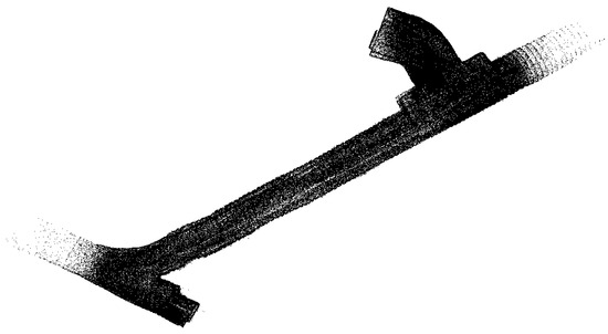
Figure 1.
Example point cloud of a mine working.
In parallel with scanning, measurements of parameters are performed and recorded every second, including pressure, temperature, relative humidity, and any other relevant measuring devices (such as multi-gas analyzers, pyrometers, etc.). The results of these measurements are also saved and integrated into a CSV file. These measurements are not strictly required. Nevertheless, they enable error control and the calculation of heat flows (sensible and latent separately for each segment). Airflow measurements are carried out in individual sidings, and in practice, they are only required in sidings with installed ventilation stoppings (where local resistance needs to be determined). Simultaneous surface measurements are no longer strictly necessary but allow for the determination of absolute potentials and make subsequent model validation easier. It should be highlighted that ensuring precise time synchronization across all measuring devices is essential.
In this case study, gas and temperature measurements were not analyzed simultaneously with the scanning, though the method supports their integration. When included, they enable the calculation of atmospheric parameter changes for individual segments and their relative variation along the analyzed section, following the same approach applied to aerodynamic resistance.
Stage III
After saving all point cloud scans and measurements to a single directory, maintaining the naming conventions adopted above, a standard Python code is launched to implement the algorithm. It locates the first scan source file and reduces it to 0.5–2% of the original point cloud (randomly removing points, reduction depending on the computer’s processing power or the original scan density). The reduced file is saved in CSV format. It then retrieves the start and end coordinates of the scans from the point array and performs transformations in the reduced point cloud space according to the procedure described below. Figure 2 illustrates the concept of transforming a spatial point cloud using a displacement vector and a rotation matrix, without the need for georeferencing markers.
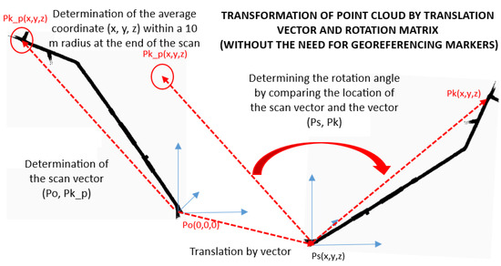
Figure 2.
Concept of point cloud transformation using a translation vector and a rotation matrix without georeferencing markers.
The left side shows the process of determining the scan vector as a segment connecting the starting point P0 = (0,0,0) with the scanning endpoint Pkp (x,y,z), averaged over points within a 10 m radius. The right side provides the current location of the point cloud from Ps (x,y,z) to Pk (x,y,z). The transformation involves first shifting the entire point cloud to the origin and then rotating it around a reference vector to reflect the local geometry of the actual tunnel. The red arrow represents the rotation according to the angle between the scan vector and the reference vector. This scheme provides the basis for automatically matching laser scanning data to the ventilation grid without the need for external georeferencing points.
The starting point (P0) in the scans is assigned to the coordinate (0,0,0), while the scan endpoint (Pkp) is determined based on the average coordinates of the last 5 s of the scan. Based on these data, the algorithm determines the translation vector from (0,0,0) to Ps (the starting coordinate of the scan read from the point table) and calculates the rotation matrix (rotation angle) of the point cloud determined by comparing two auxiliary vectors: W1 (0,0,0; Pkp) and W2 (Ps; Pk). After performing the spatial transformation of the reduced point cloud, the file is saved in the directory together with a transformation report. Based on these reports, it is possible to later perform transformations of the original high-resolution scan files without reducing them, thus avoiding quality loss.
Stage IV
The next step involved integrating the transcription commands with data from measuring instruments, including pressure, temperature, atmospheric composition, and other measurement readings. This step is unnecessary if we are not performing parallel measurements or conducting a mining inventory. This method allows for automatic application of information to equipment diagrams and comments. During scanning, the scanner’s comments can be recorded using a voice recorder. Once the recording is transcribed and saved to a file, it will recognize the need to insert a fan symbol into the diagram. In the described example, these functions were not implemented. However, this method allows for such integration.
Stage V
In this stage, the centroid of the point cloud is determined with segmentation every 1 m (can be extended to several meters). A local coordinate system (perpendicular to the local centroid) is created at the center of each segment, and local points are projected onto it. Based on these points, envelopes are created around the extreme points, examining their local “roughness” (the method for determining roughness and the FF coefficient will be described later in this paper). Figure 3 presents an example of geometric-resistance analysis for segment no. 95, performed using the new ventilation network construction method. The graph shows the projection of the point cloud (blue) onto the local cross-section plane XZ. Geometric contours are also visible: the actual outline (red), lines of matched circular sections (green, orange, purple), and the centroid (red dot). The lower part of the graph provides the cross-section characteristics: section length (1.02 m), width (4.96 m), height (3.51 m), surface area (13.52 m2), characteristic radius, as well as aerodynamic parameters—including roughness (0.36744), linear loss factor λ (0.1012), and friction factor FF (0.0152 kg/m3).
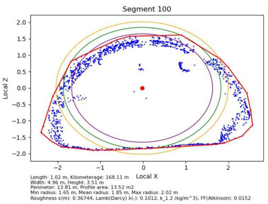
Figure 3.
Example analysis of segment No. 100 using the new ventilation network construction method.
For each subsequent segment, a similar procedure was performed, providing local point cloud cross-sections, matching contours, and geometric characteristics. This comparison allows for a prompt assessment of the excavation’s geometric variability over a longer section and the detection of local anomalies, deformations, or obstacles affecting airflow parameters and ventilation efficiency.
For each centroid, a calculation file is generated containing the following information:
- Segment No.—Number of the segment (1 m section, can be modified) in the analyzed point cloud.
- Width [m]—Maximum width of the segment profile in the local coordinate system (X-axis).
- Height [m]—Maximum height of the segment profile in the local coordinate system (Z-axis).
- Perimeter [m]—Length of the segment’s cross-sectional perimeter, calculated using the convex hull.
- Segment length [m]—Actual length of the segment, i.e., the distance between the centroids of adjacent cross-sections.
- Volume [m3]—Segment volume, calculated as the cross-sectional area multiplied by the segment length.
- Average cross-section [m2]—Average cross-sectional area of the segment.
- Chainage [m]—Distance along alignment of the segment measured from the start of the analysis.
- Roughness—Calculated as the difference between the average farthest and nearest radius for the 25% of cross-sectional points.
- Lambda (Darcy) [−]—Darcy friction factor calculated based on roughness and cross-section diameter [28].
- FF (Atkinson) [kg/m3]—Atkinson resistance factor calculated based on roughness and cross-section diameter [29].
- Farthest_Radius [m]—Average distance of the farthest 25% of points from the centroid (maximum radius).
- Closest_Radius [m]—Average distance of the nearest 25% of points from the centroid (minimum radius).
Table 3 presents a representative section of the output file containing the calculated geometric and resistance parameters for individual tunnel segments obtained with the new ventilation network construction method. For clarity, the data are shown for segments 21–34 rather than from the very beginning of the scan, since the initial and final parts of the point cloud often contain edge effects and noise that may distort parameter estimation. This results from the need to stabilize the local tunnel orientation, which is determined based on centroid points. The point cloud in the area of tunnel intersections becomes highly dispersed, leading to the generation of several to a dozen erroneous segments, depending on the cross-sectional dimensions. Consequently, during data export to VentSim, the algorithm enables the automatic removal of the first and last segments (a parameter that can be adjusted manually) or the elimination of segments whose values exceed five times the median for the corresponding data column (also user-defined). The table includes basic geometric data (average cross-section, chainage, maximum and minimum radii) as well as aerodynamic characteristics (roughness, linear resistance coefficient λ according to Darcy–Weisbach, and the Atkinson friction factor FF).

Table 3.
Example content of the file with point cloud centroid calculations in the new ventilation network construction method.
Based on the complete dataset, a 3D polyline is generated in DXF format together with the calculated parameters for each segment. This file can be directly imported into VentSim software, which automatically reconstructs the ventilation siding and assigns the cross-sectional geometry, resistance coefficients, and other ventilation attributes to the corresponding network elements.
Stage VI
Next, the point cloud is cleaned and reduced. Noise removal from the reduced point cloud is performed along the highest local average point density. A mesh is constructed based on 10% of the reduced point cloud (the mesh is constructed based on 0.05% of the original point cloud). The mesh is saved to a DXF file for visualization of the excavation in VestSim or CAD programs. Figure 4 shows the reduced point cloud and the generated model, both from the interior and exterior.
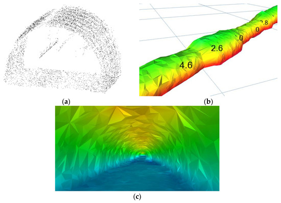
Figure 4.
View of: (a) the reduced point cloud; (b) generated model—view from outside the roadway; (c) generated model—view from inside the roadway.
2.4. Description of the Implemented Algorithm
The proposed algorithms were implemented using a custom Python script (v.3.13.7), with standardized testing procedures applied to ensure reproducibility. The algorithms automatically modify the VentSim DESIGN network file (version 6.0.4.0, 64-bit) saved as a *.txt file (the program uses .vsm by default) by locating and updating the lines that define the ventilation network structure. This process is fully automatic and opening the modified .txt file in VentSim provides complete functionality. The results are compatible with any software, as the 3D polyline coordinates and the calculated resistance coefficients, characteristic dimensions, and other parameters are simultaneously saved in an .xlsx spreadsheet. In addition to these calculations, the script generates 3D polylines annotated with calculated values (.dxf format), cross-sectional images of individual segments (.jpg format), and a report of the performed transformations and point cloud reductions (.xlsx format). The operation of the script can be divided into four fields, which are described in detail below.
Scan preparation
The script employs random downsampling algorithms to reduce the number of points while preserving a representative geometric structure of the object. Basic geometric metrics are then calculated from the coordinates, including spatial extent (diagonal length of the bounding box), point density in meters, and estimated memory usage. The program also enables export of the reduced point cloud to .csv format, accompanied by an automatically generated report detailing the processing parameters.
The script relies on the following libraries: NumPy and Pandas for numerical calculations and data processing, Open3D for 3D point cloud operations and visualization, LasPy for LAS/LAZ file support, ezdxf for DXF file handling, and PyQt5 for the graphical interface.
Transformation
The algorithm reads 3D point clouds (CSV, LAS, LAZ, PTS, PLY, or DXF formats) and, if a knots.csv file with node coordinates is provided, performs automatic georeferencing. First, points are translocated so that the scan origin aligns with node P1. The program then estimates the local excavation direction by identifying the point farthest from P1, collecting its neighbors within a 25 m radius (KD-Tree), averaging their coordinates, and deriving a direction vector. A minimum-angle rotation (Rodrigues formula) aligns this vector with P1→P2, and an optional global Z→−Z axis inversion restores the original convention of negative Z values. Manual translation and rotation are also available. For quality control, the point cloud can be visualized with coloring based on Z-value. Surface reconstruction is performed using an alpha shape derived from either the original or transformed points (user-selectable), and volumes are estimated every 10 m along the Z axis using a convex hull. The resulting surface is exported to DXF (3DFACE) with volume annotations for individual slices, and a processing report can be generated to summarize the workflow.
The script uses the following libraries: NumPy and Pandas for data handling and linear algebra, SciPy (KDTree) for neighbor search, alphashape for alpha shape reconstruction, trimesh for hull and volume calculations, Open3D for geometry operations and visualization, LasPy (LAS/LAZ I/O), ezdxf for DXF export, Matplotlib for Z-based coloring, and PyQt5 for the graphical interface.
Generating 3D polylines and calculating cross-sections
The program loads a point cloud (CSV, LAS, LAZ, PTS, or E57), divides the route along the X axis into segments of fixed length (default 1 m), and calculates the centers (centroids) and chainage of each segment. For each adjacent pair of centroids, it defines a local axis system (tunnel direction, transverse axis, and vertical), projects point within a narrow layer around the cross-section plane, and computes cross-sectional characteristics, including perimeter and area (via convex hull), width, height, and radius statistics (minimum, mean, maximum). From these metrics, the program estimates roughness (ε), friction coefficient λ (Darcy), FF (Atkinson), and section resistance. For each segment, a report with all parameters and metrics is saved to Excel, and a diagnostic cross-section plot is generated. The full centroid line is exported to DXF as a 3D polyline with text annotations of segment parameters. The algorithm accounts for short-span segments (degeneracies) and limits the analysis to points close to the section plane.
The script uses the following libraries: NumPy, Pandas, SciPy (ConvexHull), Matplotlib, LasPy, Open3D, ezdxf, and tkinter (for I/O dialogs).
Integration with VentSim
In the final step, the algorithm reads the segment table from an Excel file and a VentSim TXT file template, then automatically generates and inserts segment records between the MAIN/MINE … END MAIN/END MINE tags. Each Excel row is mapped to a single-line segment definition, including a unique GUID and all fields required to describe VentSim sidings. Before exporting, the program can optionally clean the data by removing rows with empty fields and eliminating outliers, defined as rows where any numerical value exceeds k × the median (with k user-defined). Additionally, a specified number of rows can be omitted from the top and bottom (trim head/tail) to filter out extreme segments. The output is a new TXT file representing the VentSim network, which can be opened like a standard network file, accompanied by a summary (log and report window) detailing the number of segments, cleaning actions, and deleted rows.
The script relies on the following libraries: pandas (I/O and table processing), tkinter (GUI, file selection dialogs, messages), uuid (segment identifiers), datetime (time stamps), re (text normalization), webbrowser/urllib (optional email report sketch), and the standard os/pathlib modules for file operations.
2.5. Verification of the Ventilation Model Construction Algorithm
To test the accuracy of the developed point cloud segmentation and analysis method, a synthetic tunnel model was generated (each tunnel 100 m long) with the following cross-sections:
- circular with radius r = 2 m,
- square with side a = 2 m,
- rectangular with sides a = 6 m and b = 2 m,
- trapezoidal with dimensions a = 6 m, b = 4 m, and h = 4 m,
- arched profile with simulated cavities, a = 6 m and h = 4 m.
Point clouds were randomly generated for the interior sections of the excavation profile, with an assumed scanning density of ~700–13,000 points per square meter with a tolerance of ±10 cm, which simulates the imperfections of actual laser scanning and surface irregularities. Additionally, random noise was introduced, representing 2% of the total number of points—these points were placed randomly within the tunnel cross-section. The data was saved in CSV format with x, y, and z columns, corresponding to the tunnel’s orientation along the axes. Sample sections of the generated point cloud, along with the results obtained, are shown in Figure 5.
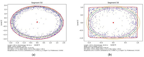
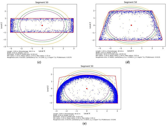
Figure 5.
Generated point cloud: (a) with a circular cross-section and radius r = 2 m; (b) with a square cross-section and side a = 2 m; (c) with a rectangular cross-section and dimensions a = 6 m and b = 4 m; (d) with a trapezoidal cross-section and dimensions a = 6 m, b = 4 m, and h = 4 m; (e) for a roadway with ŁP steel arch support (Polish standard arch support type ŁP), with voids above the support, and dimensions a = 6 m and h = 4 m.
As a result of the comparative analysis between the ideal tunnel cross-section profile generated for calculations and the results obtained by the algorithm in the new ventilation modeling method, the results shown in Table 4 and Table 5 were obtained.

Table 4.
Results of the comparative analysis of the generated point clouds simulating mine workings—point-based for segments 50—chainage 50 m.

Table 5.
Results of the comparative analysis of the generated point clouds simulating mine workings—average for the entire scan—100 m of the working (99 segments).
The smallest errors (below 0.32%) occur for circular and square profiles, which indicates good consistency of the method for simple, regular shapes. For rectangular and trapezoidal profiles, the errors are slightly higher (1.55–1.62%). The largest deviations appear for the arched profile (ŁP steel arch support) 20.52% area error. This is because voids generated in the point cloud are not accounted for in the comparison. The actual accuracy would certainly be higher, as the algorithm interprets points “captured” above the support outline as part of the free cross-section, thus increasing the calculated cross-sectional area. The roughness (ε) increases with greater profile complexity—it is lower for simple shapes and significantly higher for irregular profiles (e.g., rectangle: ε ≈ 0.62 m).
2.6. Construction of a Ventilation Model—Case Study
A ventilation siding in one of the coal mines in Poland, with a total length of 369 m, was analyzed. This side serves as a group air current conducting air to the exhaust shaft, carrying so-called used air. The roadway is constructed in ŁP steel arch support (with varying support sizes) at the 838 level (–522.8 m AMSL). The work is equipped with a KSP suspended monorail track and pipelines.
First, the accuracy of the BAR-TH barometers was calibrated relative to each other at the bottom of the mine. Calibration consisted of observing the readings of instruments located next to each other and correcting the observed values based on the noted difference. Barometers were placed at the inlet and outlet of the examined section of the excavation, and continuous recording of pressure, temperature, and humidity measurements was initiated at a 1 min interval. Simultaneously, air velocity was measured at the measuring station every 10 min using a RAW hand-held vane anemometer. Although instantaneous measurements were taken with an anemometer at a single point every minute, it was ultimately decided to rely on the results from manual measurements. In this approach, the operator uses the traverse method to measure the average velocity across the entire cross-section, rather than at a single point at frequent intervals. Barometers record data every second, but when exporting data, the records are automatically aggregated to 1 min intervals. Pressure drop and airflow were measured for 180 min. The excavation and adjacent sections were scanned with a BLK2GO device. The data were then automatically processed using the new ventilation network construction method described above. Based on the ventilation measurements, the average airflow and pressure drop were determined and compared with the results calculated using the new ventilation network construction method, which utilizes laser scanning and was visualized in VentSim software.
3. Results
The study aimed to evaluate the accuracy of the new method for constructing ventilation network models based on roadway geometry scanning and aerodynamic parameter analysis.
3.1. Measurement and Simulation Results
The variability of the pressure drop over time in the analyzed ventilation siding is shown in Figure 6. Local fluctuations in the range of approximately 160 to 260 Pa are visible, with distinct short-term drops that may indicate dynamic disturbances in the airflow.
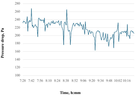
Figure 6.
Pressure drop measurement for a segment in the analyzed ventilation siding as a function of time.
A summary of the key results obtained from the measurements, along with their comparison to the simulation results from VentSim software, is presented in Table 6. The differences between reality and the model are minor, not exceeding ±5%, which confirms good model calibration and its suitability for representing real conditions. The largest difference was observed for the cross-sectional area (+5.1%), which may result from local geometric deformations that are difficult to fully reproduce in classical models.

Table 6.
Summary of results—comparison of measurements and simulation results.
The pressure drop in individual segments of the siding (from 60 to 370) determined using the Atkinson method for air with a density of 1.2 kg/m3, is shown in Figure 7. The analysis reveals significant variability in pressure losses, with sections exhibiting clearly higher local resistance, indicating areas of increased roughness or reduced cross-sectional area.
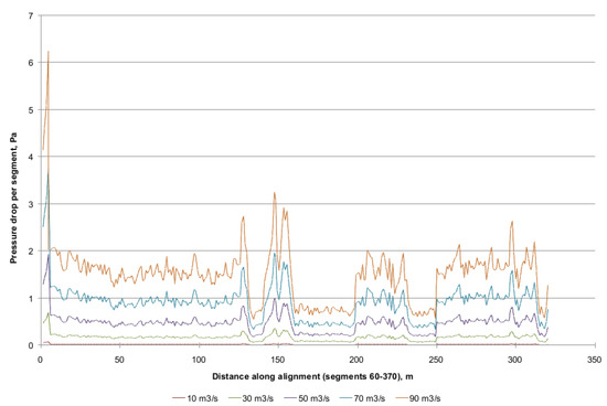
Figure 7.
Pressure drop for segments No. 60 to 370 for air density 1.2 kg/m3 based on the Atkinson method.
Figure 8 presents the resistance coefficient values: k (FF—Atkinson) and λ (Darcy) along the siding. A high stability of the coefficients is observed along most of the route, with several step changes, which may be related to the presence of deformations, obstacles, or structural changes in the roadway.
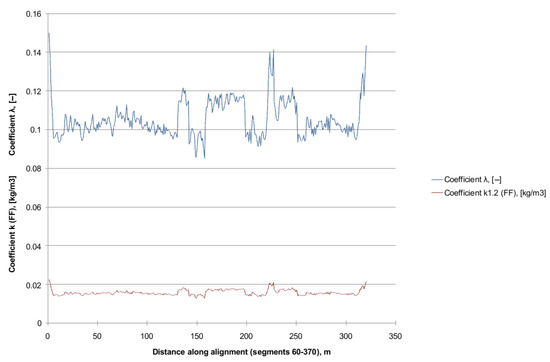
Figure 8.
Variation in the resistance coefficients: k (FF) (Atkinson) and λ (Darcy) for segments 60–370.
The variability of the roughness parameter ε and the ε/D ratio is presented in Figure 9. These values are consistent with the previous conclusions: areas with increased resistance are characterized by higher relative roughness, which directly translates into increased pressure losses in turbulent flow.
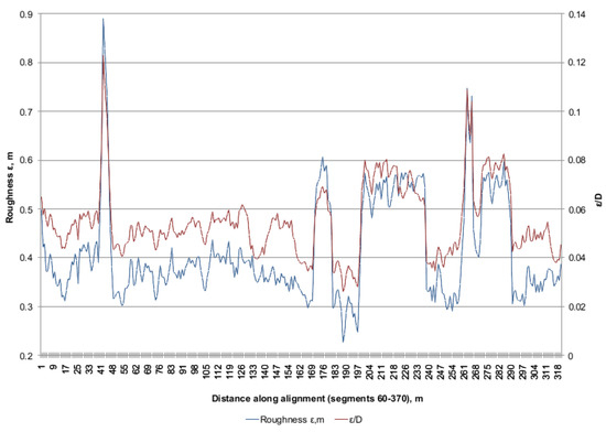
Figure 9.
Variation in roughness ε and ε/D for segments 60–370.
Figure 10 compares the pressure drop calculated using two methods (Darcy and Atkinson) for different airflow rates and air densities. A strong dependence of pressure losses on the assumed airflow volume is visible. Both methods produce comparable trends, indicating consistency, although the absolute values differ. The differences increase with higher air flow rates. For airflow rates up to approximately 61.51 m3/s, the differences remain below the typical measurement uncertainty of barometric pressure devices.
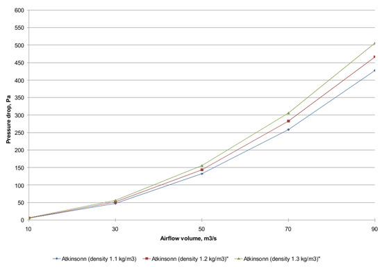
Figure 10.
Comparison of pressure drop calculations using the new ventilation network modeling method, depending on the calculation method and air density (for segments 10–242), L = 358.6 m.
Simulation results from VentSim include pressure distribution, airflow velocity, unit resistance, and flow rate (Figure 11). The results confirm a uniform distribution of the airflow (constant flow rate), as well as variations in velocity and resistanceconsistent with the results obtained from the scanning data.
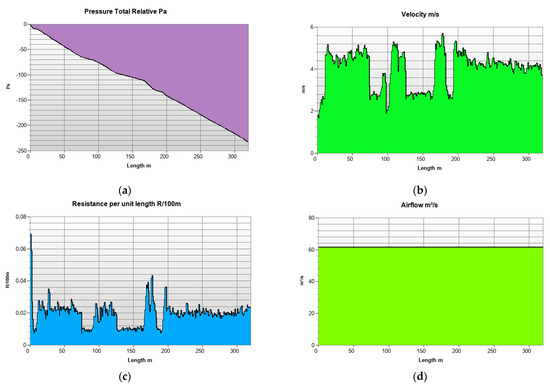
Figure 11.
Calculation results in VentSim software according to the new ventilation modeling method: (a) total relative pressure; (b) air velocity; (c) resistance per unit length (R/100 m); (d) airflow.
Figure 12 presents a three-dimensional visualization of the roadway with the siding surface represented using a triangular mesh. This visualization illustrates the actual variability of the tunnel geometry, which is crucial for roughness analysis and accurate airflow modeling.
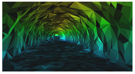
Figure 12.
Visualization of segment representation using a mesh (according to the new ventilation modeling method).
3.2. Error Analysis and Dataset Size
During the analysis of the results, the first and last 10 segments of the roadway were omitted from the presentation. This decision was made due to errors occurring at the extreme points of the point cloud (Figure 13). These errors were caused by the algorithm attempting to generate cross-sections and determine the roughness of the roadway starting from the very first points of the point cloud, where the number of points was insufficient.
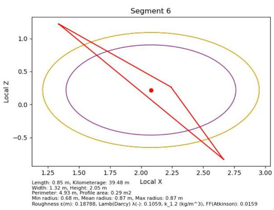
Figure 13.
Segment 6—errors in cross-section processing and roughness determination.
The error observed in the first and last meters of the scanned roadway was corrected in the description of the new ventilation network modeling method (the scan should start at the center of the roadway intersection—at the network nodes).
The original roadway scan contained 114,535,742 points in the point cloud and occupied 2184.6 MB in a LAS file. After point cloud reduction, 572,678 points remained, with a total size of 17.9 MB in a CSV file. The generated mesh based on the reduced point cloud occupied 9.6 MB in a DXF file. It can be estimated that the scan of an entire medium-sized mine (100 km) in the original (unreduced) version will take about 600 GB, while the reduced scan for roughness determination will take 5 GB, and the generated mesh will take 2.6 GB.
The calculation time on a PC (via PyCharm compiler) based on the reduced point cloud, including 3D polyline creation, cross-section generation, and roughness determination for each segment, is approximately 100 s for 369 m (≈4.0 m of roadway per second). For 100 km of roadway, the computation time is estimated at approximately 7 h.
4. Discussion
The obtained results confirm the high compliance of the new method with reality. Differences between the results obtained in VentSim and in situ measurements did not exceed ±5% for key airflow parameters. The obtained results are consistent with the observations of other authors, who emphasized the importance of considering wall roughness in the accurate modeling of flow resistance. Similar to the studies by Gao et al. [24], differences in air resistance result mainly from irregular cross-sections and additional equipment elements. Compared to classical models based solely on barometric measurements, the new method enables better representation of spatial parameter variability, because the distribution of pressure losses and roughness can be analyzed segmentally. The greatest advantage of this method is its ability to automatically transform a point cloud into a ventilation model ready for use in VentSim in a short amount of time. A full-minded length model can be obtained in a significantly shorter time compared to traditional methods requiring manual inventory. An additional advantage is the absence of the need for geolocation markers.
However, the method also has limitations. The largest errors occur with highly irregularly shaped profiles, such as arcs with voids (surface errors reached 20.52% with the ŁP model). Noticeable problems also occurred in the first and last scan segments, where the number of points was insufficient to determine the centroid and roughness correctly. Furthermore, the method assumes turbulent flow, which may limit its use in regions with low air speeds (<0.5 m/s). Ultimately, the quality of results depends on the scanner type. The critical factor is not the number of points captured by a scanner (reduced to 2–10% of the original point cloud), but rather the device’s directional drift. While geolocation and pre-processing of the point cloud could be applied before calculations, doing so would substantially increase scanning time.
During the development of the proposed approach, several areas requiring improvement and further optimization of the algorithm were identified. In particular, the effect of point cloud density on the accuracy of calculated resistance and cross-section coefficients was examined. Further research in this area is highly justified, as reducing the number of points could significantly accelerate calculations. The file formats used for data transformation also require enhancement. While the method currently supports CSV, LAS, LAZ, PTS, PLY, and DXF files, a new format appears necessary—one capable of storing not only x, y, and z coordinates but also pressure, temperature, humidity, and surface pressure variations. Standardization of such a format will be essential. Another challenge arises from the large number of analyzed points, which can create distortions during mesh generation when the dataset is too large. Short segments, typically less than approximately 30 m, also pose a problem, as the algorithm has only just stabilized the tunnel direction by the end of these segments. In such cases, the resistance determined for the central part of the excavation should be applied to the remaining short segments to ensure consistent results.
The method has significant practical potential in mining and tunneling engineering. Process automation allows for regular updates of ventilation models without the need for large measurement teams. This enables ongoing monitoring of excavation conditions and the rapid identification of areas with increased fan energy losses, helping to reduce energy costs, which in mining can account for as much as 40–50% of total ventilation costs. In the future, the method should be extended to fully integrate gas, temperature, and humidity sensors, enabling autonomous updates of databases and real-time digital mine models. It is also necessary to improve point cloud cleaning algorithms to minimize edge errors. An interesting direction is to combine the method with digital twins, which would enable ongoing optimization of fan operation and reduce methane emissions. The development of artificial intelligence can further improve resistance prediction based on geometric and environmental data.
5. Conclusions
The research demonstrated that the developed method for constructing ventilation models based on 3D scanning is an effective and practical tool for analyzing mine ventilation networks. The key feature of the proposed approach is the elimination of the need for geolocation markers and the full automation of the process of converting the point cloud into a numerical model. This allows for the rapid acquisition of input data for calculations, significantly reducing the time required to prepare a ventilation network model from days of measurement to just a few hours of computer calculations.
Comparison of the calculation results obtained using 3D scanning with actual measurements demonstrated high agreement, confirming the method’s correctness and practical utility. Differences between measured and calculated values did not exceed 5% for key airflow parameters, such as velocity, flow rate, and pressure drop. This indicates the algorithm’s high accuracy, even in complex mining conditions, where traditional approaches are affected by significant errors resulting from geometric simplifications. The method becomes particularly valuable when cross-sections are disrupted by embedded machinery, equipment, or installations, as information about their presence helps to increase the estimated roughness coefficient and, consequently, the calculated resistance. Periodic inspection of excavations allows for continuous monitoring of their condition and a more accurate determination of resistance. Unlike the currently used “potential images” of the mine ventilation network, scanning can be performed during working days because the results are not affected by factors such as pressure pulsations in the ventilation system or the movement of personnel and machinery. This approach also enables ongoing monitoring of excavation conditions, rapid identification of areas with elevated energy losses, and optimization of main fan operation.
It should be emphasized, however, that the proposed approach also has its limitations. The largest calculation errors were observed in irregularly shaped excavations, where the difference in the determined cross-sectional area could reach 15%. The discrepancy is primarily due to a different method of defining excavation dimensions. The scan-based approach considers all points situated above the excavation support. Another challenge arises from errors occurring in the first and last segments, as well as at excavation intersections, resulting from insufficient data to determine the centroids. These errors are caused by the high dispersion of the point cloud and varying scan directions, which are only confirmed in subsequent segments. They can be mitigated by automatically removing the first or last few scan segments. Increasing the length of individual segments is also possible, though this may reduce the accuracy of the reconstructed excavation shape, particularly along curves. Once exported to the software, these errors are easily identifiable and can be corrected. Another limitation is the assumption of turbulent airflow, which may be inappropriate in some regions with very low air velocities. In mine ventilation practice, this is generally not a significant concern, as studies show that the dominant flow is typically turbulent. In situations where the flow is laminar or within transitional Reynolds number zones, the resulting pressure drop in these areas is minimal. The method proposed in this article for determining ventilation siding resistance is both innovative and highly promising. Nevertheless, several aspects require further refinement to enhance its reliability, improve practical applicability, and reduce implementation time.
Based on the conducted analyses, it can be concluded that the presented method provides a valuable complement to existing ventilation modeling techniques and develops new perspectives for the development of mine digital twins. Further research should focus on integrating scanning results with mine atmosphere monitoring systems, including measurements of gas concentration, temperature, and humidity. This will enable the creation of dynamic, multi-faceted ventilation models that will support real-time decision-making. Simultaneously, algorithms for automatic point cloud cleaning and error minimization should be developed, further enhancing the accuracy and reliability of the method. In summary, the new method represents a step towards intelligent, energy-efficient, and safe underground ventilation. Its implementation in industrial practice could improve the efficiency of ventilation systems, reduce energy costs, and increase work safety in mines.
Supplementary Materials
The following supporting information can be downloaded at: https://drive.proton.me/urls/CAV594DFN4#6w1uJTtndWr7, accessed on 28 October 2025; Video S1: 3D Scanning for Mining Ventilation Systems Szmuk Andrzej.mp4.
Author Contributions
Conceptualization, A.S. and M.B.; methodology, A.S.; software, A.S.; validation, A.S. and K.Z.-G.; formal analysis, A.S., K.Z.-G. and M.B.; investigation, A.S. and K.Z.-G.; resources, A.S., M.B. and Z.K.; data curation, A.S.; writing—original draft preparation, A.S. and Z.K.; writing—review and editing, A.S., K.Z.-G. and M.B.; visualization, A.S.; supervision, M.B. and Z.K.; project administration, M.B.; funding acquisition, M.B. All authors have read and agreed to the published version of the manuscript.
Funding
This research received no external funding.
Data Availability Statement
The data supporting the findings of this study are available from the corresponding author upon reasonable request. All research results, analysis outputs, and algorithm performance videos are made available for educational and scientific purposes. However, the original underground mine point cloud scan data are not publicly shared due to JSW S.A.’s information policy, mine safety restrictions, and confidentiality agreements. The source codes used in this research are released under the Modified GNU General Public License v3 (GPLv3)—Educational and Scientific Use Only, which allows use and modification for academic and research purposes, but prohibits any commercial or industrial use without the written consent of the author (Andrzej Szmuk, 2025).
Acknowledgments
The authors would like to thank JSW S.A. for granting access to the mine workings and for technical support during the in situ measurements.
Conflicts of Interest
The authors declare no conflicts of interest.
References
- Dziurzyński, W.; Krach, A.; Pałka, T. Airflow Sensitivity Assessment Based on Underground Mine Ventilation Systems Modeling. Energies 2017, 10, 1451. [Google Scholar] [CrossRef]
- Yi, H.; Kim, M.; Lee, D.; Park, J. Applications of Computational Fluid Dynamics for Mine Ventilation in Mineral Development. Energies 2022, 15, 8405. [Google Scholar] [CrossRef]
- Kanam, O.H.; Ahmed, M.O. A Review on Underground Mine Ventilation System. J. Mines Met. Fuels 2021, 69, 62–70. [Google Scholar] [CrossRef]
- Feng, W.; Zhu, F.; Lv, H. The Use of 3D Simulation System in Mine Ventilation Management. Procedia Eng. 2011, 26, 1370–1379. [Google Scholar] [CrossRef]
- Karagianni, M.; Benardos, A. Ventilation Design Modeling and Optimization for an Underground Bauxite Mine. Mater. Proc. 2021, 5, 29. [Google Scholar] [CrossRef]
- Gyamfi, S.; Halim, A.; Martikainen, A. Development of Strategies to Reduce Ventilation and Heating Costs in a Swedish Sublevel Caving Mine—A Unique Case of LKAB’s Konsuln Mine. Min. Metall. Explor. 2022, 39, 221–238. [Google Scholar] [CrossRef]
- Jiang, A.; Zhou, B.; Hu, H.; Luan, J. Research on Mine Ventilation Optimization Based on 3D Simulation System. IOP Conf. Ser. Earth Environ. Sci. 2019, 384, 012225. [Google Scholar] [CrossRef]
- Maleki, S.; Sotoudeh, F.; Sereshki, F. Application of VENTSIM 3D and mathematical programming to optimize underground mine ventilation network: A case study. J. Min. Environ. 2018, 9, 741–752. [Google Scholar] [CrossRef]
- Zhao, C.; Cao, H.; Wan, M.; He, B.; Wu, B. Study on the influence of section shape of underground roadway on ventilation resistance. Energy Sources Part A Recovery Util. Environ. Eff. 2024, 46, 11041–11057. [Google Scholar] [CrossRef]
- Liu, Y.; Huang, D.; Li, Y. Predictive Modelling of CART-Based Frictional Resistance in Mine Ventilation Systems. Min. Metall. Explor. 2022, 39, 301–315. [Google Scholar] [CrossRef]
- Cao, P.; Liu, J.; Wang, H.; Wang, Y.; Liu, X.; Wang, D. Uncertainty analysis of digital twin model of mine ventilation system. Sci. Rep. 2024, 14, 26558. [Google Scholar] [CrossRef]
- Brovko, D.; Makareiko, R.; Sakhno, S.; Yanova, L.; Pischikova, O. Modeling the stability of air flows in inclined workings in case of fire. Min. Miner. Depos. 2024, 18, 52–62. [Google Scholar] [CrossRef]
- Nguyen, C.H.; Vu, T.T.; Le, D.T.; Do, S.A.; Dao, C.V.; Le, P.Q. Assessment of the ventilation system and solutions for improving the ventilation network at Khe Cham Coal Mine, Vietnam. Eng. J. Satbayev Univ. 2025, 147, 20–29. [Google Scholar] [CrossRef]
- Saleem, H.A.; Ali, I.; Ahmed, S. Energy Consumption Reduction in Underground Mine Ventilation. Sustainability 2025, 17, 1038. [Google Scholar] [CrossRef]
- Wróblewski, A.; Wodecki, J.; Trybała, P.; Zimroz, R. A Method for Large Underground Structures Geometry Evaluation Based on Multivariate Parameterization and Multidimensional Analysis of Point Cloud Data. Energies 2022, 15, 6302. [Google Scholar] [CrossRef]
- Zhang, H.; Mao, S.; Li, M. A Coal Mine Excavation Tunnels Modeling Method Based on Point Clouds. Appl. Sci. 2024, 14, 9454. [Google Scholar] [CrossRef]
- Dusza-Pilarz, K.; Kirej, M.; Jasiołek, J. Use of Laser Scanning and 3D Software in Mining Design. E3S Web Conf. 2024, 526, 01012. [Google Scholar] [CrossRef]
- Fahle, L.; Holley, E.A.; Walton, G.; Petruska, A.J.; Brune, J.F. Analysis of SLAM-Based Lidar Data Quality Metrics for Geotechnical Underground Monitoring. Min. Metall. Explor. 2022, 39, 1939–1960. [Google Scholar] [CrossRef]
- Niubó, M.; de Felipe, J.J.; Bascompta, M.; Pérez-Ràfols, F.; Vives-Costa, J.; Sanmiquel, L.; López, J.-A. Assessing mine ventilation optimization and friction factor determination for underground mines. Arab. J. Geosci. 2025, 18, 72. [Google Scholar] [CrossRef]
- Trybała, P.; Rigon, S.; Remondino, F.; Banasiewicz, A.; Wróblewski, A.; Macek, A.; Kujawa, P.; Romańczukiewicz, K.; Redondo, C.; Espada, F. Optimizing Mining Ventilation Using 3D Technologies. Int. Arch. Photogramm. Remote Sens. Spatial Inf. Sci. 2024, 48, 427–434. [Google Scholar] [CrossRef]
- Watson, C.; Marshall, J. Estimating underground mine ventilation friction factors from low density 3D data acquired by a moving LiDAR. Int. J. Min. Sci. Technol. 2018, 28, 657–662. [Google Scholar] [CrossRef]
- Bascompta, M.; Sanmiquel, L.; Anticoi, H.F.; Oliva, J. Ventilation friction factor determination and comparison: Two case studies of potash mining. J. S. Afr. Inst. Min. Metall. 2019, 119, 865–870. [Google Scholar] [CrossRef]
- Bascompta, M.; Sanmiquel, L.; de Felipe, J.J.; Vives, J. Friction Factors Determination of the Auxiliary Ventilation System in an Underground Mine. In Proceedings of the 5th World Congress on Mechanical, Chemical, and Material Engineering (MCM’19), Lisbon, Portugal, 15–17 August 2019. [Google Scholar] [CrossRef]
- Gao, K.; Zhipeng, Q.; Liu, Y.; Zhang, J. Calculation model for ventilation friction resistance coefficient by surrounding rock roughness distribution characteristics of mine tunnel. Sci. Rep. 2022, 12, 3193. [Google Scholar] [CrossRef]
- Zhao, C.; Wu, B.; Wang, J.; Cao, H. Calculation Method of Roadway Ventilation Resistance Based on Fractal Characterization of Wall Roughness. Phys. Fluids 2025, 37, 035137. [Google Scholar] [CrossRef]
- Brkić, D. New explicit correlations for turbulent flow friction factor. Nucl. Eng. Des. 2011, 241, 4055–4059. [Google Scholar] [CrossRef]
- Brkić, D. A note on explicit approximations to Colebrook’s friction factor in rough pipes under highly turbulent cases. Int. J. Heat Mass Transf. 2016, 93, 513–515. [Google Scholar] [CrossRef]
- Darcy, H. Les Fontaines Publiques de la Ville de Dijon: Exposition et Application des Principes à Suivre et des Formules à Employer Dans les Questions de Distribution d’eau: Ouvrage Terminé par un Appendice Relatif aux Fournitures d’eau de Plusieurs Villes, au Filtrage des Eaux et à la Fabrication des Tuyaux de Fonte, de Plomb, de Tôle et de Bitume; Dalmont, V.: Paris, France, 1856. [Google Scholar]
- Atkinson, J.J. A Practical Treatise on Friction of Air in Mines; D. Van Nostrand: New York, NY, USA, 1875. [Google Scholar]
Disclaimer/Publisher’s Note: The statements, opinions and data contained in all publications are solely those of the individual author(s) and contributor(s) and not of MDPI and/or the editor(s). MDPI and/or the editor(s) disclaim responsibility for any injury to people or property resulting from any ideas, methods, instructions or products referred to in the content. |
© 2025 by the authors. Licensee MDPI, Basel, Switzerland. This article is an open access article distributed under the terms and conditions of the Creative Commons Attribution (CC BY) license (https://creativecommons.org/licenses/by/4.0/).