Abstract
To address issues such as low visual SLAM (Simultaneous Localization and Mapping) positioning accuracy and poor map construction robustness caused by light variations, foliage occlusion, and texture repetition in unstructured orchard environments, this paper proposes an orchard robot navigation method based on an improved RTAB-Map algorithm. By integrating ORB-SLAM3 as the visual odometry module within the RTAB-Map framework, the system achieves significantly improved accuracy and stability in pose estimation. During the post-processing stage of map generation, a height filtering strategy is proposed to effectively filter out low-hanging branch point clouds, thereby generating raster maps that better meet navigation requirements. The navigation layer integrates the ROS (Robot Operating System) Navigation framework, employing the A* algorithm for global path planning while incorporating the TEB (Timed Elastic Band) algorithm to achieve real-time local obstacle avoidance and dynamic adjustment. Experimental results demonstrate that the improved system exhibits higher mapping consistency in simulated orchard environments, with the odometry’s absolute trajectory error reduced by approximately 45.5%. The robot can reliably plan paths and traverse areas with low-hanging branches. This study provides a solution for autonomous navigation in agricultural settings that balances precision with practicality.
1. Introduction
Visual SLAM serves as the foundational technology that enables mobile robots to perform autonomous localization and mapping [1] without prior knowledge of the environment [2]. Within the ROS navigation stack, it provides critical spatial information for global path planning and real-time obstacle avoidance, especially in challenging unstructured settings like orchards [2]. It captures environmental information through visual sensors, estimates the robot’s pose in real time, and constructs an environmental map [3], providing critical spatial decision-making support for autonomous navigation. Against the backdrop of rapid advancements in smart agriculture, orchards—as a quintessential setting for large-scale cultivation of cash crops [4]—are experiencing an increasingly urgent demand for automation in operations such as plant protection, inspection, and harvesting [5]. Mobile robots serve as the core execution vehicles for these tasks, and the re liability of their navigation systems directly determines operational efficiency and cost control [6]. Unlike structured environments such as indoor spaces and urban roads, or chards represent a typical unstructured scenario [7]. Their complex environmental characteristics impose higher demands on the robustness and adaptability of VSLAM technology [8].
At present, a series of mature algorithms has emerged in the field of VSLAM. The ORB-SLAM [9] series of algorithms leverages the rotation and scale invariance of ORB features, combined with local map bundle adjustment and global optimisation, to achieve high-precision pose estimation. They demonstrate outstanding performance in scenes with stable lighting and rich textures; RTAB-Map (Real-Time Appearance-Based Mapping) [10] centres on “front-end odometry, back-end map optimisation, and memory management” to generate dense 3D point cloud maps and 2D raster maps, providing excellent environmental representation for obstacle detection during navigation. Additionally, PTAM [11], SVO [12], LSD [13], and other algorithms have also demonstrated advantages in feature extraction efficiency and computational resource adaptation, driving the application of VSLAM in structured environments [14]. However, these algorithms still face significant limitations in the unstructured environment of orchards: On one hand, or chards feature variable lighting conditions, dense foliage obstruction, and highly repetitive ground textures [15], causing traditional VSLAM algorithms to suffer from pose drift. On the other hand, while high-precision algorithms like ORB-SLAM3 can produce stable poses, their sparse feature point maps cannot directly support the dense obstacle detection required for navigation [16].
In practical orchard applications, VSLAM technology primarily faces three core challenges. First, positioning accuracy and mapping robustness are insufficient. Due to drastic changes in lighting and the absence of repeated textures on fruit trees [8], visual odometers are prone to pose estimation errors, which in turn compromise the consistency of the global map. Secondly, there is a mismatch between environmental representation and navigation requirements. Sparse maps lack obstacle information [3], while unprocessed dense maps tend to introduce numerous false obstacle points, making it difficult to accurately describe the navigable space within orchards [17]. Thirdly, navigation systems suffer from poor integration. A single SLAM algorithm typically struggles to independently complete the entire closed-loop process from pose estimation and map construction to path planning, necessitating collaboration with mature navigation frameworks [18].
In recent years, a fusion approach combining a high-precision SLAM front-end with a dense mapping back-end has provided a solution to the aforementioned issues [19]. This approach employs a SLAM algorithm specialised in pose estimation as the front-end visual odometry, combined with a navigable map back-end processing framework [20]. This ensures trajectory accuracy while generating more practical environmental maps [20]. To address typical disturbances such as low-lying branches and foliage in orchards, a para metric point cloud filtering strategy effectively removes noise [21], generating maps more suitable for navigation. Against this backdrop, this paper investigates a navigation method based on an improved RTAB-Map algorithm to address the autonomous navigation requirements of orchard robots.
The main work of this paper is as follows:
1. The RTAB-Map algorithm framework was enhanced by integrating ORB-SLAM3 as the visual odometry module. Leveraging its local map optimisation and bundle adjustment capabilities, this approach improves pose estimation accuracy in complex orchard environments, reduces cumulative error, and provides reliable pose support for dense mapping.
2. Propose a point cloud filtering strategy based on height thresholds, setting appropriate parameters during post-processing to eliminate interference from low-lying branches and foliage while preserving critical information such as tree trunks and ground surfaces. This generates a two-dimensional raster map with enhanced navigational value.
3. An orchard navigation system was developed by integrating the ROS Navigation framework with the A* global path planning algorithm, utilising the TEB local obstacle avoidance method to achieve autonomous navigation. In simulated orchard experiments, the improved system demonstrated enhanced visual odometry accuracy and path planning reliability.
2. Related Work
2.1. Visual SLAM Techniques for Unstructured Environments
Visual SLAM is the core technology enabling mobile robots to achieve self-localization and map construction in unseen environments. In unstructured environments such as orchards and farmlands, where lighting conditions fluctuate dramatically and scene textures exhibit high repetitiveness [22], the robustness and accuracy of SLAM systems face significant challenges.
Early SLAM solutions were predominantly based on filtering theory, such as MonoSLAM [21] and frameworks utilising Extended Kalman Filters (EKF). Their computational complexity increases dramatically with map scale, making them unsuitable for mapping large-scale orchards. In recent years, keyframe-based and graph optimisation-based approaches have become mainstream [23], such as PTAM and the ORB series. Among these, the ORB-SLAM series has gained widespread adoption due to its outstanding positioning accuracy and robustness. It employs ORB (Oriented FAST and Rotated BRIEF) feature points, which combine rotation and scale invariance with high computational efficiency, making it suitable for operation on embedded platforms with limited computational resources. The standard ORB-SLAM3 primarily generates sparse feature point maps, which are suitable for localization but difficult to directly apply to navigation tasks requiring dense obstacle information.
To obtain dense maps suitable for navigation, solutions such as RTAB-Map have been proposed. RTAB-Map typically employs visual or laser odometry as its front-end sensors, with its core comprising back-end image optimisation and memory management mechanisms. It is capable of generating dense 3D point clouds and 2D raster maps with colour information in real time. Its original visual odometry is prone to failure during rapid motion or when textures are absent. Therefore, by integrating a high-performance visual SLAM system as the odometry front-end with an RTAB-Map back-end focused on mapping and closed-loop verification, this study adopts this approach by replacing the odometry module of RTAB-Map with ORB-SLAM3, aiming to achieve both high-precision pose estimation and high-quality dense map construction.
2.2. Map Representation and Navigation Map Construction in Orchard Environments
How to transform perceived data into a map representation suitable for path planning is fundamental to navigation tasks [18]. In agricultural applications, two-dimensional grid maps (2D Grid Map) are most commonly used due to their high computational efficiency and excellent compatibility with mainstream navigation frameworks such as the ROS Navigation Stack [24]. It divides the environment into occupied, free, and un known areas using the grid-occupancy algorithm.
Standard two-dimensional raster maps compress three-dimensional point clouds onto a two-dimensional plane, rendering them incapable of representing or processing obstacle information in the vertical space [25], such as low-hanging branches of fruit trees. This may cause the robot to plan paths that appear collision-free on the ground projection SF but are actually impassable in reality. To address this issue, researchers typically employ two strategies: First, constructing 2.5D elevation maps or 3D voxel maps [26], but such maps incur significant computational and storage overhead; another more efficient strategy involves filtering out irrelevant obstacles during the point cloud pre-processing stage by setting a height threshold [27]. By setting an appropriate Z-axis range, the system preserves major obstacles like tree trunks while filtering out lower branches and foliage, generating a “passable” two-dimensional navigation layer map. This study adopted the latter strategy, effectively addressing spatial obstacles within orchard canopies by integrating the filtering capabilities of RTAB-Map with custom parameters.
3. Method
3.1. Principles of the RTAB-MAP Algorithm and Its Improvements
RTAB-Map is a graph-based SLAM method widely used in RGB-D SLAM, employing depth data to build 3D point cloud maps for robot navigation. To adapt it to orchard environments—which contain numerous low-hanging, traversable branches and foliage—we enhance the conventional RTAB-Map framework in two ways. First, we integrate ORB-SLAM3 to supply high-precision pose estimates in place of RTAB-Map’s native visual odometry, improving estimation robustness and accuracy. Second, we apply a height filtering strategy at the point cloud level to produce navigation-tailored maps that eliminate unnecessary overhead obstacles. The overall improved architecture is illustrated in Figure 1.
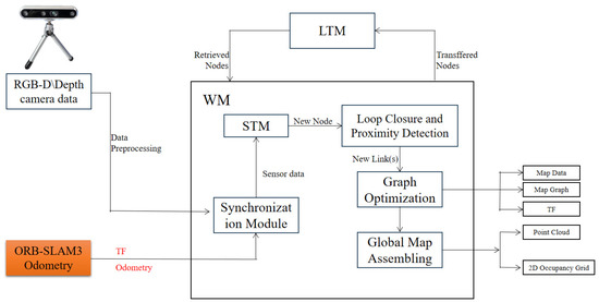
Figure 1.
Overall system framework.
The inputs for the improved RTAB-Map algorithm comprise two primary components: depth camera data and external visual odometry data provided by ORB-SLAM3. Depth camera data is provided in RGB-D format; external visual odometry data is sup plied by the ORB-SLAM3 system, with its pose information published via the nav_msgs/Odometry message type. The coordinate frames of all sensors are unified with that of the robot chassis using the TransformFrame (TF) mechanism. A detailed temporal flow of the entire system is illustrated in Figure 2, showing the data exchange between ROS nodes and the sequential processing from input synchronisation to planning. The system TF tree is shown in Figure 3.
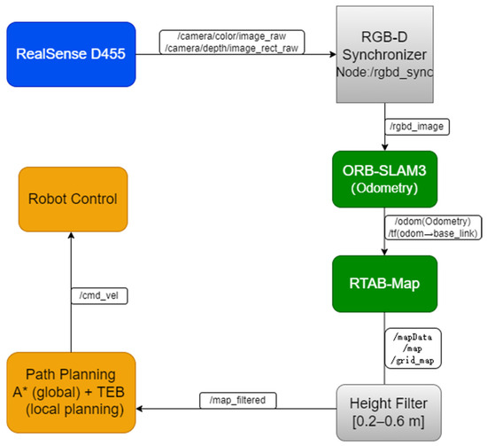
Figure 2.
System Temporal Flow Diagram.

Figure 3.
The system TF tree.
As pose data and image data are input into the system asynchronously via different topics, timestamp alignment processing is required. The data synchronisation process is illustrated in Figure 4. Employ the rgbd_sync node to precisely synchronise the image and depth information from the RGB-D camera, ensuring they share identical timestamps. The aligned RGB-D data is then approximately synchronised with the pose information released by ORB-SLAM3 to ensure consistency between environmental perception and pose estimation data. For synchronising RGB-D images (rgbd_sync) and external odometry data, the message_filters::ApproximateTimepolicy was employed. This policy matches messages from different topics based on their timestamps within a defined temporal tolerance (slop). A queue size of 10 messages per topic was used to buffer incoming data while searching for timestamp matches across topics. The slopparameter was set to 0.05 s, defining the maximum allowable time difference between timestamps for messages to be considered synchronised.
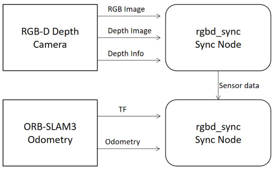
Figure 4.
Sensor Data Synchronisation Process.
Synchronised sensor data is stored within the Short-Term Memory (STM) module. This module primarily creates nodes for each frame of data and stores them.
The external visual odometry system provides core pose estimation information for constructing local maps. Based on the node pose information provided by ORB-SLAM3, the local maps are stitched together to form a global map. In this study, ORB-SLAM3 provides only visual odometry functionality, without performing its original loop closure detection and global optimisation. This design prevents conflicts with RTAB-Map’s backend graph-optimisation module and ensures that the odometry-generated pose sequence remains continuous and smooth. This facilitates the proper functioning of backend loop closure detection and graph optimisation.
The workflow of ORB-SLAM3, employed as an external visual odometry module, consists of the following key stages: First, the system receives colour and depth image inputs from the RGB-D camera and extracts ORB feature points from each frame. The ORB feature comprises the FAST corner detector and the BRIEF descriptor, exhibiting both rotation and scale invariance. It is well-suited for robust feature detection in orchard environments characterised by varying illumination and repetitive textures. During the feature matching phase, ORB-SLAM3 performs nearest neighbour matching on ORB descriptors from adjacent frames and resolves ambiguities using Lowe’s ratio test. The de termination formula for reliable feature matching is given in Equation (1):
and denote the Hamming distances between a feature point and its nearest neighbour and second-nearest neighbour, respectively. When the ratio is less than the threshold , the match is deemed reliable. During the pose estimation phase, ORB-SLAM3 establishes 3D-2D correspondences based on matched point pairs, and solves the camera pose using PnP (Perspective-n-Point) and RANSAC. As formulated in Equation (2):
Here, denotes a three-dimensional point, represents its observed pixel in the image, is the camera projection function, and is the robust kernel function (used to suppress the influence of anomalous matching points). Upon obtaining the initial pose, ORB-SLAM3 further employs nonlinear optimisation (Levenberg–Marquardt, LM) to minimise reprojection error, thereby achieving a higher-precision pose. To enhance the stability of short-term tracking, ORB-SLAM3 performs local bundle adjustment (BA) within the local keyframe window, defined in Equation (3):
and denote the camera pose at frame , represents a point in the 3D map, and indicates the observation correspondence. In this study, the loop closure detection module of ORB-SLAM3 was disabled, and its candidate frame retrieval functionality based on DBoW2 visual bag-of-words no longer participated in pose estimation. This ensured that only smooth, continuous visual odometry results were published to the /odom topic in ROS.
Ultimately, the odometry messages issued by ORB-SLAM3 are passed as external input to RTAB-Map, replacing its internal RGB-D odometry algorithm. The accuracy and robustness of front-end pose estimation have been significantly enhanced, whilst loop closure detection and global map optimisation continue to be performed by the RTAB-Map backend. The system thus achieves a balance between high-precision odometry and the retention of dense mapping capabilities alongside global consistency optimisation. ORB-SLAM3 serves as an external odometry framework, as illustrated in Figure 5. As shown in Appendix A.1, these are the key parameters for ORB-SLAM3 as a visual odometry system.
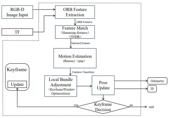
Figure 5.
ORB-SLAM3 Odometry Framework.
Furthermore, additional closed-loop detection and global optimisation of the global map are required. Within the RTAB-Map algorithm, closed-loop detection is achieved through a visual bag-of-words model and a Bayesian filter. The visual bag-of-words model updates the weight of a localisation point by calculating the similarity between the current pose node and the working memory (WM) node, thereby determining whether the node participates in closed-loop detection or is transferred to the long-term memory (LTM) module. In this approach, the backend optimiser of RTAB-Map performs loop closure correction and global optimisation based on the precise initial pose provided by ORB-SLAM3. This ultimately outputs a high-quality navigation map that is globally consistent and free from invalid high-altitude obstacles.
Within this integrated research system, although the front-end pose is provided by the high-precision ORB-SLAM3, significantly reducing cumulative error, the back-end global optimisation remains crucial for ensuring map consistency in large-scale environments. The closed-loop detection and optimisation module of RTAB-Map is re sponsible for executing this task. Closed-loop detection is achieved through the collaborative operation of a visual bag-of-words model and a Bayesian filter. The bag-of-words model converts images into vectors composed of visual words, rapidly screening loopback candidate frames by comparing vector similarity. For the current pose node and the historical node in the working memory (WM), the similarity between their bag-of-words vectors is computed using Equation (4).
In the formula: and denote the total number of visual words in the current node and the candidate node, respectively, while represents the number of matched word pairs. This similarity metric ensures the fairness and validity of the matching process.
However, mere visual similarity is susceptible to perceptual ambiguity (such as repetitive visual structures within a garden). Consequently, the system employs Bayesian filtering to estimate the probability of closed-loop existence, thereby comprehensively determining the most probable feedback node. Let denote the aggregate state of all candidate feedback nodes at time “”. Its probability distribution is updated via Bayes’ theorem, as in Formula (5):
In the formula: denotes the normalisation constant, represents the observation likelihood computed via Equation (4), and signifies the state transition probability. Through continuous updating, the candidate node with the highest prob ability shall be confirmed as the correct loop. Upon successful detection of the closed loop, this constraint is incorporated into a pose graph. The system invokes optimisers such as g2o to perform global optimisation on all pose nodes within the graph (initialised with high-precision poses provided by ORB-SLAM3). This effectively corrects any residual mi nor drift from the front-end, yielding a globally consistent optimal pose estimation. Upon completion of optimisation, the locally mapped areas associated with each node are fused, ultimately generating a globally consistent map for navigation purposes.
3.2. Post-Processing Raster Map Optimisation Methods for Orchard Scenes
Autonomous navigation within orchard environments frequently encounters challenges in practical application due to low-hanging branches, shrubbery, and irregular terrain, leading to the emergence of ‘false obstacles’ during robot mapping and path planning. Conventional vision-based mapping methods, when generating two-dimensional occupancy grid maps, often misinterpret low-level branch point clouds as obstacles capable of impeding robot movement. This misinterpretation consequently triggers path de tours or planning failures. To address this issue, this paper proposes a post-processing method for point cloud height filtering, thereby enhancing the robustness and feasibility of robotic operations within orchard environments. This method optimises the rasterisation parameters within the database file (rtabmap.db) generated following RTAB-Map mapping, thereby achieving precise modelling of passable terrain. Considering the typical weed height in orchards, the overall height of the orchard navigation robot (H = 42.5 cm), and potential future configurations such as mounting robotic arms, this study opts to remove point cloud data within the range . The specific procedure is as follows: Configure the key parameters of the Grid module within the .db file: Grid/MaxGround Height: 0.6; Grid/MinGroundHeight: 0.2. The key parameters for RTAB-Map and modifications to key parameters within the .db file are shown in Appendix A.2.
The three-dimensional point cloud of low-hanging branches in the simulated orchard scene is shown in Figure 6. The red box indicates branches that may not impede the navigation of orchard robots within the scene, yet their projections onto the two-dimensional grid map are classified as obstacles. As shown in Figure 7, the point cloud under goes high-pass filtering to specifically eliminate interference from low-hanging branches during navigation. Only key navigational information—such as tree trunks, ground sur faces, and low-lying obstacles—is retained.
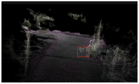
Figure 6.
Simulated three-dimensional point cloud map of an orchard.
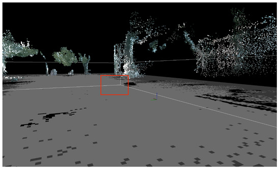
Figure 7.
Height-filtered three-dimensional point cloud map.
The processed point cloud data is converted into the robot coordinate system via the TF tree, generating the corresponding two-dimensional raster map. This is further optimised within the ROS Navigation framework to refine the cost map. Finally, stable autonomous navigation within complex orchard environments is achieved through the combined application of A* and TEB path planning algorithms. Mathematically, this process can be defined as Formula (6):
Here, denotes the original point cloud set, while represents the filtered point cloud, with . Through this approach, low-hanging branches and foliage within the 0.2–0.6 m height range are effectively removed, whilst obstacles above ground level that genuinely impede the robot’s passage remain preserved. The filtered occupancy grid map is thus rendered more concise, providing a more accurate representation of the environment for subsequent path planning.
In the realm of navigation path planning, this study employs a combined approach utilising the global path planning algorithm A* alongside the local path planning method TEB (Timed Elastic Band). The global A* path planning cost function is expressed in Equation (7).
where denotes the cumulative cost from the starting point to the current node, and represents the heuristic estimate from the current node to the destination, typically taken as the Euclidean distance. The A* algorithm guarantees the connectivity and optimality of the global path, providing constraints for the robot’s overall motion direction. However, A* alone is insufficient for handling dynamic obstacles or accommodating the robot’s kinematic constraints. Therefore, this paper further introduces the TEB algorithm as a local planner. TEB decomposes the global path into a series of time-constrained trajectory bands. Through nonlinear optimisation, it simultaneously considers trajectory smoothness, dynamic feasibility, and obstacle avoidance constraints. The TEB optimisation objective is formulated in Equation (8), balancing trajectory smoothness, dynamic feasibility, and obstacle avoidance cost.
denotes a trajectory point, with the first term constraining trajectory continuity and the second term maintaining obstacle avoidance via a cost map, where serves as the balancing coefficient. During optimisation, TEB dynamically adjusts its path based on real-time sensor inputs, thereby achieving flexible obstacle avoidance in semi-structured environments such as orchards. By integrating a hierarchical strategy combining global A* and local TEB, the robot maintains overall path optimality while possessing the capability to avoid low-hanging branches and root obstacles in real time.
The aforementioned strategy ensures the accuracy of environmental representation through processed maps, while cost map optimisation enhances parameter consistency between mapping and navigation phases. The integration of A* and TEB balances global optimality with local dynamic feasibility, thereby enabling the robot to maintain stable autonomous navigation capabilities within complex orchard environments. The principal parameters used for the local TEB planner and costmap configuration are summarised in Appendix A.3 These parameters define the motion limits, obstacle avoidance constraints, and Ackermann kinematic restrictions of the robot, ensuring dynamic feasibility and safe navigation in the orchard environment.
4. Experiments and Analysis
4.1. Experimental Platform
This study evaluated the enhanced RTABmap system through a real-world simulated orchard scenario. Performance metrics include absolute path error (APE) and relative pose error (RPE) for assessing global positional accuracy. This experiment employed artificially simulated dwarf fruit trees with drooping branches and foliage within the test area. The experiment utilised a robot equipped with an Ackermann steering system driven by a DC motor, featuring an Intel Core i5-12450H (2.00 GHz) processor and 16 GB of memory. The robot operated on the Ubuntu 18.04 operating system and was integrated with the Robot Operating System (ROS) Melodic. The host computer established communication with the chassis via a USB-to-serial converter module, operating at a baud rate of 115,200. The system implementation employed ORB-SLAM3 (v0.4), RTAB-Map (v0.20.23), g2o (20201223_git), and OpenCV (3.4.3), with the Intel RealSense D455 running firmware version 5.13.0.50. This study employs the Intel RealSense D455 depth camera as its core environmental perception sensor. This device is an active stereo vision camera integrating an RGB global shutter colour camera, two infrared stereo imaging modules, and an infrared laser projector. It synchronously outputs high-resolution colour imagery alongside depth point cloud data. Its depth perception range offers high precision between 0.5 and 6 m, with a maximum range exceeding 10 m. Featuring a field of view (FOV) of 86° × 57°, it provides SLAM algorithms with rich visual and geometric information.
The camera connects to the host computer via a USB 3.0 interface and is powered through this connection. RGB images and depth stream data are sampled simultaneously at approximately 30 Hz. During data acquisition, the robot records raw data from the visual sensors into ROS Bag files. These files serve as input for the offline processing stage, where an enhanced RTAB-Map SLAM algorithm is executed on the AGV robot to con struct a dense three-dimensional point cloud map and a two-dimensional grid map of the environment. The experimental platform is illustrated in Figure 8.
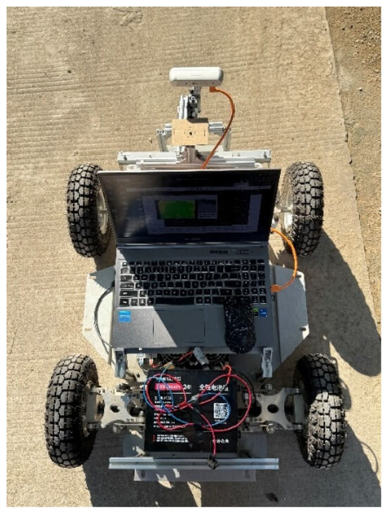
Figure 8.
Orchard Navigation Robot.
4.2. Experimental Validation
4.2.1. Visual Odometry Error Analysis
To validate the stability of the developed orchard navigation robot and the effectiveness of the fused odometry, the robot was controlled to traverse an approximate elliptical trajectory with a perimeter of approximately 24 m at a speed of 0.20 m per second. For quantitative assessment and comparison of positioning accuracy among SLAM algorithms. In this study, the ground-truth trajectory was obtained using the LIO-SAM system, which fuses LiDAR and inertial measurements to produce high-precision pose estimates with centimetre-level drift in short-range outdoor environments. The LIO-SAM trajectory was recorded simultaneously with the visual data and used as the reference for evaluating the ORB-RTAB and baseline RTAB-Map results. To ensure consistency, all trajectories were temporally aligned using ROS timestamps and spatially registered via a similarity transformation estimated by the EVO alignment module. The enhanced RTAB-Map was designated as ORB-RTAB. Performance analysis was conducted on trajectories generated by the ORB-RTAB algorithm and those produced by RTAB-Map as an external odometry output. The EVO evaluation tool was employed to analyse the positioning performance of both algorithms. Key metrics examined were absolute pose error (APE) and relative pose error (RPE), with a comprehensive assessment conducted across two dimensions: global consistency and local smoothness.
To visually demonstrate algorithmic performance, Figure 9 presents a two-dimensional plane comparison of the three trajectories. It can be observed that when employing the improved odometry for path planning, the robot’s motion trajectory closely aligns with the target trajectory. Conversely, when using the original odometry for planning, significant deviation occurs between the robot’s trajectory and the target trajectory at turning points. In the simulated orchard scenario, both methods closely matched the ground truth. However, at path junctions, the RTAB-Map trajectory exhibited more pronounced drift, with a significantly greater offset than the ORB-RTAB trajectory. This result preliminarily suggests that ORB-RTAB may offer greater robustness in pose estimation when employed as a visual odometry.
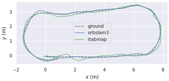
Figure 9.
Movement Trajectory of Orchard Navigation Robot.
Absolute positional error (APE) is employed to assess the global consistency of trajectories. The APE time-series curve in Figure 10 further illustrates the fluctuating trends of the two curves, where the error curve of RTAB-Map exhibits higher peaks at multiple time points. This correlates with the drift phenomenon observed at turning points in Figure 9. Statistical analysis of the APE for the translation component (Table 1) indicates that ORB-RTAB outperforms RTAB-Map across all key metrics.
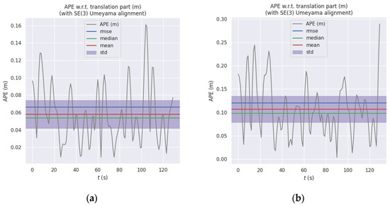
Figure 10.
Comparison of Absolute Path Error (APE) between ORB-RTAB and RTAB-Map: (a) APE curve of ORB-RTAB as odometry; (b) APE curve of RTAB-Map with built-in odometry.

Table 1.
Statistical Comparison of Absolute Pose Error (APE).
As shown in Table 1, the RMSE of the absolute pose error (APE) for ORB-RTAB (0.066 m) was reduced by approximately 45.5% compared to RTAB-Map (0.121 m), with its maximum error decreasing by 44.3%. This fully demonstrates that ORB-RTAB can consistently provide pose estimates closer to the true values throughout the entire motion process.
Relative pose error (RPE) is employed to evaluate the precision of local motion. The statistical results in Table 2 clearly demonstrate that ORB-RTAB exhibits a significant advantage in local motion accuracy when used as a visual odometry. Figure 11a,b illustrate the temporal variation in inter-frame relative pose error. The statistical findings align with the APE conclusions: ORB-RTAB’s mean RPE (approximately 0.022 m) and standard deviation (Std) are both lower than those of RTAB-Map. This indicates that ORB-RTAB not only achieves greater accuracy in global pose estimation but also demonstrates superior smoothness and stability in continuous inter-frame motion estimation.
Table 2.
Statistical Comparison of Relative Position Error (RPE).
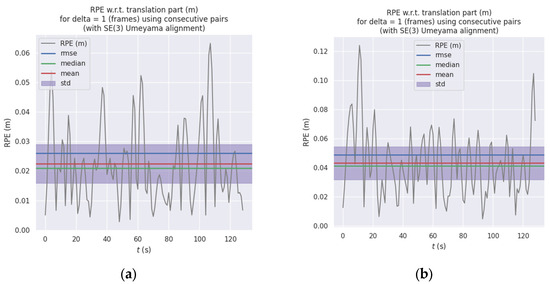
Figure 11.
Comparison of Relative Position Error (RPE) between ORB-RTAB and RTAB-Map: (a) RPE curve of ORB-RTAB as odometry (b) RPE curve of RTAB-Map with built-in odometry.
Experimental results demonstrate that, within this experimental scenario, employing ORB-RTAB as an external odometry source yields comprehensively superior performance compared to directly utilising the raw trajectory generated by RTAB-Map. ORB-RTAB, leveraging its superior feature point extraction and matching algorithms, demonstrates greater robustness when confronting challenges such as lighting variations and repetitive scene textures, thereby achieving higher positioning accuracy. However, as a comprehensive SLAM framework, RTAB-Map integrates global optimisation and closed-loop detection capabilities, which prove crucial for suppressing cumulative error during prolonged, large-scale operations.
4.2.2. Map Construction and Navigation Experiments
To validate the effectiveness of the proposed improved RTAB-Map algorithm for mapping and robot navigation in simulated orchard environments, experiments were conducted at a test site within the North China University of Water Resources and Electric Power. The experimental setup is illustrated in Figure 12. All experiments were conducted on a clear, sunny afternoon (around 4:00 P.M.). The Intel RealSense D455 camera (Intel Corporation, Santa Clara, CA, USA) was operated with its default auto-exposure and auto-gain settings enabled to adapt to the natural lighting conditions. The robot was re motely controlled via Bluetooth to traverse the simulated orchard environment for two complete laps. The internal reference for RealRense D455 is as per Appendix A.4.
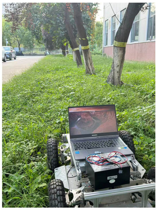
Figure 12.
Simulation Experiment for Orchard Navigation Scenario Mapping.
In this experiment, we employed an enhanced RTAB-Map for fusion mapping to generate a 2D raster map of the orchard environment. As shown in Figure 12, the initial map ping results depict light grey areas as navigable space and black patches as obstacles. However, several black patches appear in the map (red-boxed regions in Figure 13), corresponding to the projection of low-hanging branches and foliage onto the 2D raster map within the simulated orchard environment. In reality, these low-hanging branches do not impede the robot’s passage beneath them. Nevertheless, the irregular distribution of these foliage projections disrupts the map’s accurate representation of the actual ground scene, thereby diminishing both the map’s usability and the reliability of navigation.
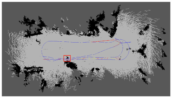
Figure 13.
Map generation results for simulated orchard scenario.
Following the processing of the database (.db) file after mapping with the improved RTAB-Map as described in Section 3.2, the three-dimensional points projected onto the two-dimensional raster map after removing the effects of low-hanging branches are shown in Figure 14. It can be observed that after eliminating the low-hanging branches depicted in Figure 13, key information such as tree trunks remains preserved.
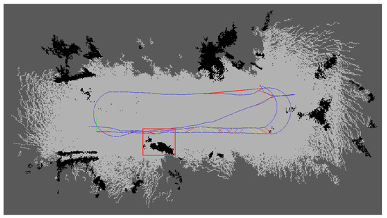
Figure 14.
Post-processing results of the two-dimensional raster map.
Figure 13 and Figure 14 were imported into ROS Navigation as prior maps for navigation experiments. The robot’s starting point was marked as F and the destination as G, requiring the robot to move from point F to point G. The navigation experiment is illustrated as shown. The A* algorithm generated a global path from point F to G within the cost map. TEB calculated the robot’s motion trajectory and strategy based on visual odometry data, autonomously guiding the robot towards the target location. As depicted in Figure 15, during navigation using the unprocessed grid map, the robot exhibits obstacle avoidance behaviour by treating low-hanging branches as obstacles. However, when navigating with the processed grid map, the robot traverses safely beneath the branches. Ultimately, it successfully reaches the destination point, completing the navigation task. To validate the navigational stability and computational efficiency of the system employing filtered maps, a total of 20 experiments were conducted. The system demonstrated consistent performance, achieving an average navigation time of 14 s and an average path length of 5.63 m. Regarding safety, the average and maximum vertical distances from overhead obstacles were recorded as 0.53 m and 0.58 m, respectively, indicating secure passage beneath tree canopies. Only a single path replanning was required across all trials, highlighting the high quality of global path planning and the effectiveness of the local planner. This robust navigation performance was underpinned by the computational platform. Critical modules—including the visual odometry module (12.5 ms), local planner (8.5 ms), and cost map up date (25 ms)—operated with low latency, while total CPU utilisation remained around 65%. This demonstrates substantial computational headroom on the embedded platform.
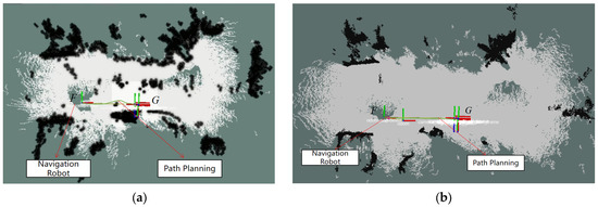
Figure 15.
Navigation Experiment in Simulated Orchard Scenario (a) Navigation experiments without high-pass filtering (b) Navigation experiment employing high-pass filtering.
The height-filtering interval of [0.2 m, 0.6 m] was chosen for sensitivity analysis to balance three objectives: (1) to avoid incorrectly removing actual ground surfaces and low-lying obstacles, thereby preserving perception of genuine hazards; (2) to effectively eliminate spurious obstacles caused by low-hanging vegetation and shadows, thus improving the accuracy of navigable space estimation; and (3) to maintain a safety margin for the robot’s own height (H = 0.425 m). Three intervals, designated as ‘aggressive’ ([0.15 m, 0.5 m]), ‘balanced’ ([0.2 m, 0.6 m]), and ‘conservative’ ([0.25 m, 0.7 m]), were evaluated. We conducted 10 autonomous navigation trials for each of the three filtering intervals. The system successfully navigated a minimum vertical clearance of 0.48 m. The results of this sensitivity analysis are summarised in the Table 3.
Table 3.
Sensitivity Analysis of Different Height-Filtering Intervals.
5. Conclusions
This study proposed an improved orchard robot navigation framework that integrates ORB-SLAM3 as the front-end odometry within the RTAB-Map system and introduces a height-constrained point-cloud filtering strategy to better reflect the traversable space in unstructured orchard environments. The combination of A* for global planning and TEB for local trajectory optimisation ensures both path optimality and real-time adaptability to obstacles and Ackermann kinematic constraints. Extensive experiments in a simulated orchard confirmed that the proposed system significantly enhances mapping consistency, localization accuracy, and navigation reliability compared with the baseline RTAB-Map configuration.
Quantitatively, the ORB–RTAB front end reduced the Absolute Pose Error (APE) by approximately 45.5% relative to the baseline odometry, demonstrating marked improve ment under conditions of variable lighting and repetitive textures. The height-filtered maps effectively removed spurious obstacles caused by low-hanging foliage while pre serving genuine traversable areas, leading to safer and more efficient path planning. The combined A*–TEB strategy enabled the robot to follow collision-free paths with smooth local adjustments, achieving stable navigation even under dense canopy coverage.
Beyond these contributions, this research emphasises the importance of tightly cou pling accurate front-end visual odometry with adaptive environmental representation and dynamic planning for agricultural robots operating in visually complex and cluttered spaces. The system effectively balances ORB-SLAM3’s precision and RTAB-Map’s loop-closure optimisation, forming a computationally efficient and robust solution suitable for embedded deployment.
Future research will focus on extending the system’s robustness and generalizability across diverse real-world orchard conditions. Specifically, we will:
- Evaluate performance under varying illumination, including day–night transitions and strong shadow variations, to improve visual stability and perception consistency.
- Expand testing to natural orchards with uneven terrain and flexible vegetation, ad dressing the influence of soil irregularity, wind-blown branches, and occlusion.
- Develop terrain-aware and contact-risk mapping modules, combining 3D voxel reasoning and density-based “contact risk” indicators to further enhance navigation safety.
- Conduct comprehensive benchmarking against other representative algorithms such as Gmapping, ORB-SLAM2, and recent agricultural navigation frameworks, to provide a broader quantitative comparison.
In summary, the proposed ORB–RTAB-based navigation framework provides a practical and accurate solution for autonomous operation in unstructured orchards. The demonstrated improvements in localization accuracy, map usability, and navigation robustness lay a solid foundation for next-generation agricultural robots, paving the way for reliable, intelligent, and fully autonomous navigation in visually complex field environments.
Author Contributions
Conceptualization, J.N. and L.Z.; methodology, J.N. and L.Z.; software, L.Z. and J.G.; validation, L.Z., T.Z., J.G. and S.S.; writing—original draft preparation, J.N. and L.Z.; writing—review and editing, T.Z. and S.S. All authors have read and agreed to the published version of the manuscript.
Funding
This work was supported by Henan Province Key Research and Development Special Project under Grant No. 231111112700, Training Plan for Young Backbone Teachers in Colleges and Universities in Henan Province under Grant No. 2021GGJS077, and North China University of Water Resources and Electric Power Young Backbone Teacher Training Project under Grant No. 2021-125-4.
Institutional Review Board Statement
Not applicable.
Informed Consent Statement
Not applicable.
Data Availability Statement
The raw data supporting the conclusions of this article will be made available by the authors on request.
Conflicts of Interest
The authors declare no conflicts of interest. The funders had no role in the design of the study; in the collection, analyses, or interpretation of data; in the writing of the manuscript, or in the decision to publish the results.
Appendix A
Appendix A.1
Table A1.
ORB-SLAM3 Concrete parameters.
Table A1.
ORB-SLAM3 Concrete parameters.
| Parameter Name | Value | Description |
|---|---|---|
| ORBextractor.nFeatures | 1000 | Number of ORB features extracted per image, balancing tracking stability and computational load |
| ORBextractor.nLevels | 8 | Number of levels in the pyramid, enhancing adaptability to scale changes |
| ORBextractor.iniThFAST | 20 | Initial threshold for FAST corner detection; higher values result in sparser features |
| ORBextractor.minThFAST | 7 | Minimum threshold for FAST detection, used as a fallback for low-contrast images. |
| BA Window Size | 10 | Bundle adjustment window size (in frames); controls local optimisation scope |
| Sensor Mode | RGB-D | Uses RGB-D mode with depth data fusion |
Appendix A.2
Table A2.
RTAB-Map Concrete parameters.
Table A2.
RTAB-Map Concrete parameters.
| Parameter Name | Value | Description |
|---|---|---|
| Grid/MaxGround Height | 0.6 | Maximum height (metres) for ground points in grid map. |
| Grid/MinGround Height | 0.2 | Minimum height (metres) for ground points. |
| Mem/RehearsalDistance | 10 | Distance for memory rehearsal; optimises loop closure detection efficiency. |
| Kp/DetectorStrategy | 2 | Keypoint detector strategy |
| Vis/FeatureType | 2 | Feature type for visual matching |
Appendix A.3
Table A3.
TEB and Costmap Configuration Parameters.
Table A3.
TEB and Costmap Configuration Parameters.
| Category | Parameter | Value | Description |
|---|---|---|---|
| TEB Parameters | acc_lim_x | 0.2 | Maximum acceleration in the x-direction (m/s2) |
| acc_lim_y | 0 | Maximum acceleration in the y-direction (m/s2) | |
| max_vel_x | 0.5 | Maximum x-forward ve locity (m/s) | |
| max_vel_y | 0 | Maximum y-forward velocity (m/s) | |
| min_obstacle_dist | 0.25 | Minimum clearance from obstacles (m) | |
| Costmap Parameters | resolution | 0.05 | Map grid resolution (m/cell) |
| inflation_radius | 0.7 | Radius of inflation around obstacles (m) | |
| obstacle_range | 2.5 | Maximum range to consider obstacles (m) | |
| raytrace_range | 3.0 | Maximum ray tracing range (m) |
Appendix A.4
Table A4.
Binocular camera stereo calibration results.
Table A4.
Binocular camera stereo calibration results.
| Parameter Type | Calibration Results |
|---|---|
| Internal parameters of colour cameras | |
| Internal Parameters of Left Infrared Camera | |
| Internal Parameters of the Right Infrared Camera | |
| Distortion coefficient of the left camera | |
| Distortion coefficient of the right camera | |
| Rotation Matrix | |
| Translation matrix |
References
- Xian, K.; Liu, D.; Zhang, G.; Neri, F.; Chen, S. Gravity-Constrained Simultaneous Localization and Mapping for suppressing map warping in complex large-scale environments. Integr. Comput.-Aided Eng. 2025, 32, 229–243. [Google Scholar] [CrossRef]
- Chen, K.; Xiao, J.; Liu, J.; Tong, Q.; Zhang, H.; Liu, R.; Zhang, J.; Ajoudani, A.; Chen, S. Semantic Visual Simultaneous Localization and Mapping: A Survey. IEEE Trans. Intell. Transp. Syst. 2025, 26, 7426–7449. [Google Scholar] [CrossRef]
- Wijayathunga, L.; Rassau, A.; Chai, D. Challenges and Solutions for Autonomous Ground Robot Scene Understanding and Navigation in Unstructured Outdoor Environments: A Review. Appl. Sci. 2023, 13, 9877. [Google Scholar] [CrossRef]
- El-Ansary, D.O. Smart Farming and Orchard Management: Insights and Innovations. Curr. Food Sci. Technol. Rep. 2025, 3, 10. [Google Scholar] [CrossRef]
- Mohyuddin, G.; Khan, M.A.; Haseeb, A.; Mahpara, S.; Waseem, M.; Saleh, A.M. Evaluation of Machine Learning Approaches for Precision Farming in Smart Agriculture System: A Comprehensive Review. IEEE Access 2024, 12, 60155–60184. [Google Scholar] [CrossRef]
- Yang, L.; Li, P.; Qian, S.; Quan, H.; Miao, J.; Liu, M.; Hu, Y.; Memetimin, E. Path Planning Technique for Mobile Robots: A Review. Machines 2023, 11, 980. [Google Scholar] [CrossRef]
- Cao, G.; Zhang, B.; Li, Y.; Wang, Z.; Diao, Z.; Zhu, Q.; Liang, Z. Environmental mapping and path planning for robots in orchard based on traversability analysis, improved LeGO-LOAM and RRT* algorithms. Comput. Electron. Agric. 2025, 230, 109889. [Google Scholar] [CrossRef]
- Hussain, I.; Han, X.; Ha, J.-W. Stereo Visual Odometry and Real-Time Appearance-Based SLAM for Mapping and Localization in Indoor and Outdoor Orchard Environments. Agriculture 2025, 15, 872. [Google Scholar] [CrossRef]
- Campos, C.; Elvira, R.; Rodríguez, J.J.G.; Montiel, J.M.M.; Tardós, J.D. ORB-SLAM3: An Accurate Open-Source Library for Visual, Visual–Inertial, and Multimap SLAM. IEEE Trans. Robot. 2021, 37, 1874–1890. [Google Scholar] [CrossRef]
- Labbé, M.; Michaud, F. RTAB-Map as an open-source lidar and visual simultaneous localization and mapping library for large-scale and long-term online operation. J. Field Robot. 2019, 36, 416–446. [Google Scholar] [CrossRef]
- Klein, G.; Murray, D. Parallel Tracking and Mapping for Small AR Workspaces. In Proceedings of the 2007 6th IEEE and ACM International Symposium on Mixed and Augmented Reality, Nara, Japan, 13–16 November 2007; pp. 225–234. [Google Scholar] [CrossRef]
- Forster, C.; Pizzoli, M.; Scaramuzza, D. SVO: Fast semi-direct monocular visual odometry. In Proceedings of the 2014 IEEE International Conference on Robotics and Automation (ICRA), Hong Kong, China, 31 May–7 June 2014; pp. 15–22. [Google Scholar] [CrossRef]
- von Gioi, R.G.; Jakubowicz, J.; Morel, J.-M.; Randall, G. LSD: A Fast Line Segment Detector with a False Detection Control. IEEE Trans. Pattern Anal. Mach. Intell. 2010, 32, 722–732. [Google Scholar] [CrossRef]
- Xu, H.; Liu, X.; Liu, Y.; Song, X. Motion Estimation and Reconstruction for 360° Panoramic Images Based on Variant Goldberg Polyhedral Projection. IEEE Trans. Intell. Transp. Syst. 2025, 26, 4891–4907. [Google Scholar] [CrossRef]
- Anthony, B.M.; Minas, I.S. Optimizing Peach Tree Canopy Architecture for Efficient Light Use, Increased Productivity and Improved Fruit Quality. Agronomy 2021, 11, 1961. [Google Scholar] [CrossRef]
- Xiao, Y.; Li, B.; Xu, W.; Zhou, W.; Xu, B.; Zhang, H. Optimization of a Dense Mapping Algorithm with Enhanced Point-Line Features for Open-Pit Mining Environments. Appl. Sci. 2025, 15, 3579. [Google Scholar] [CrossRef]
- Syed, T.N.; Zhou, J.; Lakhiar, I.A.; Marinello, F.; Gemechu, T.T.; Rottok, L.T.; Jiang, Z. Enhancing Autonomous Orchard Navigation: A Real-Time Convolutional Neural Network-Based Obstacle Classification System for Distinguishing ‘Real’ and ‘Fake’ Obstacles in Agricultural Robotics. Agriculture 2025, 15, 827. [Google Scholar] [CrossRef]
- Tang, Y.; Zhao, C.; Wang, J.; Zhang, C.; Sun, Q.; Zheng, W.; Kurths, J. Perception and navigation in autonomous systems in the era of learning: A survey. IEEE Trans. Neural Netw. Learn. Syst. 2022, 34, 9604–9624. [Google Scholar] [CrossRef]
- Chen, W.; Wang, X.; Gao, S.; Shang, G.; Zhou, C.; Li, Z.; Xu, C.; Hu, K. Overview of Multi-Robot Collaborative SLAM from the Perspective of Data Fusion. Machines 2023, 11, 653. [Google Scholar] [CrossRef]
- Al-Tawil, B.; Hempel, T.; Abdelrahman, A.; Al-Hamadi, A. A review of visual SLAM for robotics: Evolution, properties, and future applications. Front. Robot. AI 2024, 11, 1347985. [Google Scholar] [CrossRef] [PubMed]
- Davison, A.J.; Reid, I.D.; Molton, N.D.; Stasse, O. MonoSLAM: Real-time single camera SLAM. IEEE Trans. Pattern Anal. Mach. Intell. 2007, 29, 1052–1067. [Google Scholar] [CrossRef] [PubMed]
- Zhao, Z.; Wu, C.; Kong, X.; Li, Q.; Guo, Z.; Lv, Z.; Du, X. Light-SLAM: A Robust Deep-Learning Visual SLAM System Based on LightGlue Under Challenging Lighting Conditions. IEEE Trans. Intell. Transp. Syst. 2025, 26, 9918–9931. [Google Scholar] [CrossRef]
- Liu, Z.; Li, Z.; Liu, A.; Shao, K.; Guo, Q.; Wang, C. LVI-Fusion: A Robust Lidar-Visual-Inertial SLAM Scheme. Remote Sens. 2024, 16, 1524. [Google Scholar] [CrossRef]
- Zhao, K.; Ning, L. Hybrid Navigation Method for Multiple Robots Facing Dynamic Obstacles. Tsinghua Sci. Technol. 2022, 27, 894–901. [Google Scholar] [CrossRef]
- Xue, G.; Li, R.; Liu, S.; Wei, J. Research on Underground Coal Mine Map Construction Method Based on LeGO-LOAM Improved Algorithm. Energies 2022, 15, 6256. [Google Scholar] [CrossRef]
- Guo, S.; Hu, Y.; Xu, M.; Liu, J.; Ju, Z. A Novel Hybrid 2.5D Map Representation Method Enabling 3D Reconstruction of Semantic Objects in Expansive Indoor Environments. IEEE Trans. Autom. Sci. Eng. 2025, 22, 9636–9650. [Google Scholar] [CrossRef]
- Wang, P.; Gu, T.; Sun, B.; Huang, D.; Sun, K. Research on 3D Point Cloud Data Preprocessing and Clustering Algorithm of Obstacles for Intelligent Vehicle. World Electr. Veh. J. 2022, 13, 130. [Google Scholar] [CrossRef]


Disclaimer/Publisher’s Note: The statements, opinions and data contained in all publications are solely those of the individual author(s) and contributor(s) and not of MDPI and/or the editor(s). MDPI and/or the editor(s) disclaim responsibility for any injury to people or property resulting from any ideas, methods, instructions or products referred to in the content. |
© 2025 by the authors. Licensee MDPI, Basel, Switzerland. This article is an open access article distributed under the terms and conditions of the Creative Commons Attribution (CC BY) license (https://creativecommons.org/licenses/by/4.0/).