Abstract
Reliable schedule-risk estimation in hybrid software development lifecycles is strategically important for organizations adopting AI in software engineering. This study addresses that need by transforming routine process telemetry (CI/CD, SAST, traceability) into explainable, quantitative predictions of completion time and rework. This paper introduces an integrated probabilistic model of the hybrid software development lifecycle that combines Generalized Evaluation and Review Technique (GERT) network semantics with I-AND synchronization, explicit artificial-intelligence (AI) interventions, and a fuzzy treatment of epistemic uncertainty. The model embeds two controllable AI nodes–an AI Requirements Assistant and AI-augmented static code analysis, directly into the process topology and applies an analytical reduction to a W-function to obtain iteration-time distributions and release-success probabilities without resorting solely to simulation. Epistemic uncertainty on critical arcs is represented by fuzzy intervals and propagated via Zadeh’s extension principle, while aleatory variability is captured through stochastic branching. Parameter calibration relies on process telemetry (requirements traceability, static-analysis signals, continuous integration/continuous delivery, CI/CD, and history). A validation case (“system design → UX prototyping → implementation → quality assurance → deployment”) demonstrates practical use: large samples of process trajectories are generated under identical initial conditions and fixed random seeds, and kernel density estimation with Silverman’s bandwidth is applied to normalized histograms of continuous outcomes. Results indicate earlier defect detection, fewer late rework loops, thinner right tails of global duration, and an approximately threefold reduction in the expected number of rework cycles when AI is enabled. The framework yields interpretable, scenario-ready metrics for tuning quality-gate policies and automation levels in Agile/DevOps settings.
1. Introduction
1.1. Motivation
We first outline the motivation and contributions. Section 1.2 then surveys prior work and explicitly enumerates the gaps this paper addresses.
Modern software development processes are increasingly becoming hybrid. Agile practices are combined with DevOps automation, CI/CD pipelines, and continuous operational feedback. Such integration increases the speed of delivery of incremental and quality transparency, but at the same time complicates the cause-and-effect structure of the life cycle. Parallel branches of work, I-AND synchronization of artifacts (alignment of system design with UX), local and macro loops of rework (reviews, integration retests, acceptance returns), as well as strategic returns after a possible negative effect. As a result, traditional linear representations of the process are insufficient for reliable planning of deadlines and risks, as they do not reflect the probabilistic nature of decisions and iterations in a hybrid SDLC.
An additional dimension of complexity is the rapid introduction of artificial intelligence (AI) tools into some critical points of the development contours. These tools already demonstrate practical benefits, but their effect is mainly recorded in the form of empirical observations or local quality metrics. There is no formal process model that quantitatively links the use of AI to the probabilities of branching, the intensity of loops, and, ultimately, to the distributions of the timing of the likely completion of iterations and the success of releases. It is precisely this causal–quantitative relationship that managers and teams need for a well-founded choice of practices, “quality gates” policies, and the level of automation. A separate problem is uncertainty in the early stages. Incomplete knowledge of the subject area, heterogeneity of sources of requirements, different maturity of teams, and changes in external constraints. In practice, this manifests itself in a large variability of work durations and return probabilities, which is not reduced to aliatory (actually stochastic) variability.
This work focuses on hybrid software development lifecycles and explicitly considers the growing role of AI in software engineering as a first-class driver of branching, rework, and quality-assurance decisions.
Filling the outlined gap by constructing an integrated network model based on GERT, which naturally operates with probabilistic transitions and allows for the reduction in cycles to an equivalent W-function, is one of the ways to solve the above problems.
1.2. State of the Art
To reduce repetition, we use these five strands as a thematic map and synthesize shared strengths and limitations before the detailed paper-by-paper discussion.
The analysis of the literature allowed us to form a number of separate areas of the analyzed topic and to highlight the most relevant ones:
- (1)
- The general relevance of hybrid management () in software development
- (2)
- Modeling and prototyping of the software development process
- (3)
- Features of GERT modeling
- (4)
- Consideration of AI in SDLC graph models (requirements, code analysis, tracing)
- (5)
- Consideration of uncertainty: fuzzy/stochastic network models of projects
It is advisable to start the literature review with the article [1], which provides a systematic review of the integration of Agile, cloud technologies, and DevOps. This article summarizes the benefits and barriers of combining practices. The positive side of the work is the wide sample and the isolation of integration barriers. However, it does not consider formal probabilistic modeling of a hybrid SDLC with branches/cycles and AI nodes. In addition, there is no quantitative assessment of the impact of AI assistants and CI/CD loops on project timing/success.
In article [2], the authors proposed an Agile Project Management framework outside of IT, emphasizing scalability and versatility. The positive side of the article is the conceptual expansion of the applicability of agile approaches. However, stochastic modeling of work routes and quality rework is not presented. Accordingly, the impact of AI assistants in requirements and code analysis on the probability of a successful release is not taken into account.
In the article [3], approaches to Agile hybrid scaling (scaling and combining practices) are systematized. The authors consider a detailed map of hybridization options. However, the lack of a formal model of the prototyping cycle (System design blueprint → UX) and feedback loops, as well as an analytical assessment of deadlines and risks, does not allow obtaining a complete information portrait of this work and exploring its practical benefits.
While hybrid works clarify goals, cadence and flow constraints, turning these insights into operational decisions requires explicit process representations. The next group reviews modeling and prototyping approaches that map activities, artifacts, and feedback paths to support scenario analysis.
The authors of the article [4] empirically show that human factors (team competencies, customer involvement) have the greatest impact on the success of Agile projects. At the same time, the authors prove an empirical evidence base. However, the article lacks a description of a process model that links these factors to branching probabilities, rework cycles, and automated AI quality controls.
In the article [5], a generalized Petri-net framework for modeling complex service IT processes is proposed. The model developed by the authors contains a strict formalization of competition and resources. This significantly increased the reliability of the results obtained. However, probabilistic routes typical of hybrid SDLC (branches “accepted/for revision”, CI/CD rollbacks), and explicit AI nodes are not taken into account.
In the article [6], an object-oriented Petri net framework with logic programming for “smart” simulations is presented. One of the positive aspects of this scientific work is the expressiveness and integration of logic. However, the article does not calculate the finite equivalent arc (W-function) for estimating the distributions of time/success over the network, and there is no I-AND synchronization of artifacts (for example, parallel: System design blueprint + UX model). This somewhat narrows the practical significance of the study and allows for its further improvement.
The co-authors of the article [7] analyzed metrics for Software Process Simulation Modeling (SPSM) and formed a catalog of cause-and-effect metrics. However, the article does not show the transition from metrics to analytical probabilistic estimates of time and success of the final product, as well as to a formal consideration of the impact of AI.
In the article [8], stochastic Petri nets for the evolution of an online process (real cases) are implemented. A positive factor of this work was the verification of data and the use of modern knowledge in the theory of nonlinear dynamics in the work. However, the lack of modeling of SDLC prototyping (UX/interface) and DevOps loops as probabilistic branches with return probabilities reduces the practical value of the results. In addition, neglecting the capabilities of AI also reduces the reliability of the final result.
Generic process models (BPMN/UML/DES, Petri-net variants, SPSM) enable “what-if” analysis and empirical grounding, yet scaling branching with rework loops and merge semantics benefits from a network formalism with analytic leverage. We therefore turn to GERT, which natively represents branching/feedback and provides network-level moments via the W-function.
SPSM spans discrete-event, system-dynamics, and agent-based simulation to explore “what-if” scenarios in development and QA pipelines. Branching and feedback loops are native, and I-AND synchronizations are modeled via Petri-net/BPMN semantics or simulation gateways. However, calibration is often scenario-tuning rather than statistically grounded on operational telemetry, and results are simulation statistics rather than closed-form moments. Explainability is typically at the scenario/policy level (resources, WIP, rules), with parameter interpretability depending on model fidelity.
Process Mining (PM) discovers, checks, and enhances process models from event logs, yielding Petri-net/BPMN structures that expose branching, loops, and parallel gateways/joins (including AND-joins). Conformance and variant analytics provide fine-grained explainability (bottlenecks, deviations). Modern PM integrates ML/AI for predictive monitoring (e.g., risk or remaining time), but the emphasis is descriptive/predictive rather than a calibrated generative model with explicit stochastic semantics; closed-form network moments are not provided, and what-if analysis is indirect.
The authors of the article [9] derived an optimization model of the trade-off “time–cost” in GERT networks with probabilities and characteristic functions. The rigorous mathematics of the trade-off calculation allowed the authors of the article to achieve the modeling goal. However, the model does not consider the quality loops typical for SDLC (code review, static analysis, CI/CD) and AI nodes, as well as I-AND synchronization of project artifacts. Adding these elements would allow us to obtain the distributions of terms and the probability of release success.
The co-authors of the scientific paper [10] designed a GERT model for optimizing value streams under resource constraints. The positive part of the work was the consideration of resources and the value stream. However, the developed model lacks an application map for the SDLC stages (requirements → architecture → UX → code → QA → deployment) and the impact of AI controls on the probability of returns.
In the paper [11], a fuzzy-neutrosophic GERT for complex graphs is proposed. One of the achievements of this paper is the modern integration of GERT with fuzzy elements for uncertainty. However, the paper does not consider the SDLC domain and AI-specificity (requirements quality, static code analysis) with the corresponding loop probabilities.
With GERT providing structure and tractable moments for hybrid SDLCs, the next question is how AI interventions (requirements assistants, static analysis, tracing) change route probabilities and effective durations. The following works embed such AI nodes into process graphs.
The authors of the article [12] systematically reviewed requirements engineering for AI systems (frameworks, processes, tools). The article developed a map of Requirements Engineering (RE) practices for AI. However, a graph stochastic SDLC model with explicit AI assistant nodes and calculation of the impact on risks that exist in the software development process was not proposed.
The paper [13] formulates a roadmap for combining formal methods and LLM in RE. This is one of many papers that consider the use of AI methods in the process of formalization and software development, and focuses on the verifiability of LLM applications. However, the lack of process modeling of the entire SDLC as a stochastic graph with I-AND synchronization and DevOps cycles somewhat affects the accuracy of the final result.
The authors of [14] proposed an LLM approach for generating tracing relationships of requirements to code components (in particular, security traces). The article provides examples of practical tracing of natural-language requirements into code models. However, it is not shown how such AI nodes change the probabilities of returns and reworks, as well as deadlines in the software life cycle.
In [15], a comparison of classical SAST analyzers with LLM approaches was made based on repository and vulnerability level characteristics. The comparable empirical design and industrial focus allowed the authors to achieve the set goal. However, the article does not provide a process model of the propagation of the effects of static analysis on patch loops, releases, and the overall probability of success.
Reported AI effects reduce rework rates and fix times, but their magnitude is uncertain and context dependent. We therefore consider fuzzy/stochastic treatments that model epistemic and aleatory uncertainty and support sensitivity analysis and scenario calibration.
The authors of [16] combined fuzzy-PERT and Monte–Carlo to analyze network projects with uncertainties. As the authors emphasize, the positive side of this work is the correct work with fuzzy durations. However, the model does not take into account GERT-branching with the probabilities of failures and returns, characteristic of SDLC. The authors also did not consider the influence of AI-nodes.
In the article [17], a fuzzy method of linear, repeated scheduling (ASCE) is proposed. One of the factors of scientific novelty in this work was the possibility of progress in taking into account the variability of durations. However, the absence of a general stochastic network with branches (and not only linear and repeated operations) and the neglect of taking into account AI quality controls narrows the practical significance of the results.
The authors of the article [18] considered multi-project planning under uncertainty and limited resources. The most important positive feature of this work was the possibility of a systemic view of risk aggregation. However, the article has no connection with the hybrid SDLC and lacks AI nodes and DevOps loops as sources of stochastic returns.
The literature review revealed a significant gap between conceptual works on hybrid software development management and a formal probabilistic model of the entire lifecycle, capable of simultaneously reflecting branching, rework cycles, and mutual synchronization of parallel artifacts. Despite progress in the use of Petri nets, stochastic approaches, and fuzzy-PERT, either simulative or local formulations prevail, focusing on individual aspects of the process and not providing analytical generation of time distributions, assessment of the probability of release success, and sensitivity of key parameters. An additional limitation was the fragmented nature of AI. AI assistants in requirements engineering and static code analysis are more often considered as support tools, rather than as elements of the process network that change the probabilities of returns, the structure of CI/CD loops, and, ultimately, the time and quality indicators of the release. Similarly, ways of dealing with epistemic uncertainty are mostly limited to fuzzy task durations and are rarely combined with the branching, synchronization of results, and reflective loops inherent in a hybrid SDLC.
Generalizing these observations leads to the need for a single stochastic model of the hybrid development process that analytically links the quality of requirements, architectural solutions, UX prototyping, development, quality control, and deployment, enables the formal inclusion of AI nodes, and supports fuzzy-stochastic parameterization.
Collectively, these gaps motivate the research objectives stated in Section 1.1 (Motivation).
1.3. Objectives and Contribution
The aim of the research is to build a holistic stochastic model of the hybrid software development life cycle that reproduces realistic process dynamics, taking into account branches, rework loops, and synchronization of parallel artifacts. Within the framework of this aim, a formal introduction of explicit AI nodes into the process network is envisaged.
The conceptual basis is the GERT model with support for I-AND synchronization between architectural design and UX design; the analytical reduction in such a network is designed to provide W-function derivation, time distributions, release success probability estimation, and sensitivity analysis to CI/CD loop parameters and input artifact quality.
The scientific contribution of the work lies in the formation of a single and consistent with the practice of software engineering network model, capable of simultaneously reflecting stochastic branching, reflective rework loops, and I-AND synchronization of artifacts, as well as in the formal inclusion of AI nodes as elements of a process network with a quantitatively determined impact on time and quality metrics.
The results include:
- −
- Construction of an integrated stochastic SDLC model
- −
- Derivation of a closed-form network transfer function
- −
- Interpretable sensitivity analyses
We unify analytical and simulation modeling with an explicit AI node:
Analytical GERT reductions (W-function–based moments) complement Monte–Carlo distributions.
An AI-assisted static-analysis node injects telemetry signals into branch probabilities via a calibrated logistic + isotonic mapping.
Rework loops and implicit AND (I-AND) joins are handled with conservative semantics and robustness checks.
A reproducible telemetry-to-parameter pipeline (CI/CD, SAST, traceability) yields explainable, path-level attributes and closed-form summaries where available.
An additional component of the contribution is the combination of stochastic branching with fuzzy parameterization for consistent consideration of epistemic uncertainty in the parameters of nodes and arcs, as well as a reproducible calibration and empirical verification methodology that demonstrates the practical benefits of AI-support, CI/CD cycles, and UX prototyping in hybrid software development processes and creates a basis for further comparative studies with Petri nets and fuzzy-PERT in industrial scenarios.
The rest of the paper is organized as follows. Section 2 presents the mathematical model and the telemetry-to-parameter calibration pipeline. Section 3 reports the experimental results and unified quantitative summaries. Section 4 discusses limitations and threats to validity. Section 5 concludes and outlines future work.
2. Materials and Methods
2.1. Generalized Model of a Software Development Team
Analysis of modern research and practices in the field of project management has shown that the success of software development largely depends not only on the choice of methodology, but also on the organization of team interaction. In the works [19,20], it is emphasized that the effectiveness of Agile approaches is due to a well-thought-out team structure, a balanced composition, and a clear distribution of roles. At the same time, the integration of AI tools, automation, in particular CI/CD pipelines, as well as DevOps practices, allows you to significantly reduce risks and accelerate the delivery of increments.
For clarity and consistency, we consolidate all symbols and units in a single place. Table 1 lists the notation adopted in the paper and the default units used in figures and tables.

Table 1.
Notation and units used throughout.
Given the above, it is advisable to formulate a generalized team model that reflects the main roles of participants and stages of interaction in the software development process. Such a model is presented below and visualized in Figure 1.
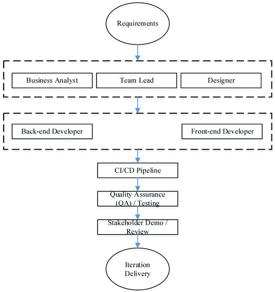
Figure 1.
Generalized model of a software development team.
The presented team structure can reflect traditional and flexible approaches, ensuring both systematic planning and flexibility in responding to changing requirements. The model presented is the result of a generalization of modern industry practices and takes into account key roles that ensure the full development cycle.
One of the important principles is to maintain a balanced team size. This helps maintain effective communication, reduces management costs, and allows for a harmonious combination of different competencies.
Within such an organization, the following roles are distinguished:
- −
- Business Analyst (Requirements Analyst)—defines and formalizes the customer’s business needs, transforming them into technical specifications. His activities reduce the risk of misinterpretation of requirements and deviation from strategic goals.
- −
- Team Lead (technical manager)—responsible for architectural decisions, code quality, and coordination of the team. In addition to technical leadership, he serves as a facilitator, resolving organizational obstacles and promoting adherence to Agile principles.
- −
- Designer (interface and user experience designer)—shapes the appearance and logic of user interaction with the system. His contribution guarantees not only functionality, but also ergonomics and competitiveness of the product.
- −
- Back-End Developer (server-side developer)—implements business logic, data processing mechanisms, and interaction with external services. This role ensures the stability and scalability of the system.
- −
- Front-End Developer (client-side developer)—responsible for creating the user interface, integrating with business logic, and implementing interactivity.
- −
- CI/CD Pipeline (automated integration and delivery pipeline) is a critical element of the modern development process, ensuring the continuity of integration, testing, and deployment of a software product. Using CI/CD allows you to quickly detect defects, accelerate the release of increments, and increase the reliability of releases.
- −
- Quality Assurance—verifies the functionality, performance, and safety of a product. Their job is to detect errors early and minimize the risk of critical failures during operation.
- −
- Stakeholder Demo/Review (presentation of results to customers and stakeholders)—the stage where the team presents the developed increment, receives an assessment of compliance with requirements and recommendations for further development.
- −
- Iteration Delivery (incremental delivery) is the final phase of iteration, which ensures continuous enhancement of system functionality and forms the basis for subsequent cycles.
2.2. Hybrid Project Management Algorithm with AI Elements
Having summarized the structure of the development team, it is advisable to move from the organizational description to the operational outline of the process, “from the concept of functionality to the delivery of the increment”. For further formalization in GERT terms, a representative process diagram is required, which clearly reflects the control conditions for decision-making, addressable feedback loops, as well as modern IT practices. First of all, a CI/CD pipeline, the separation of automated and manual quality checks, and the optional involvement of AI tools to reinforce individual steps. The updated functionality development life cycle diagram agreed upon by us (see Figure 2) serves as a reference model for further mathematical description: its nodes and transitions are further interpreted as vertices and arcs of the GERT network with the corresponding probabilities of passage from node to node, as well as duration distributions.
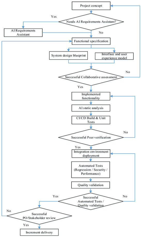
Figure 2.
Block diagram of the hybrid project management algorithm with AI elements.
Drawing on [21,22] and Agile/DevOps practices, we present a detailed description of the updated feature development flow consistent with the figure. The model reflects the iterative nature of development, combining the classic phases of analysis, design, implementation, and verification with modern automation tools (CI/CD) and decision-making checkpoints, and also supports addressable rework loops.
The life cycle begins with the conceptualization stage (Project concept), which articulates the business value and expected effects of the new functionality. Then, if necessary, the AI Requirements Assistant is involved as an auxiliary tool to clarify formulations, identify contradictions, and prepare initial usage scenarios. The use of AI is not a mandatory phase of the flow. It acts as an amplifier of the quality of requirements, not a separate mandatory step. The result of this block is the Functional specification. This is a formalized description of the requirements with acceptance criteria, non-functional constraints, and assumptions. It is the only source of truth for subsequent work.
Based on an agreed specification, two complementary design lines are deployed in parallel.
The first is the System design blueprint. It covers the choice of architectural solutions, component interaction contracts, security policies, and data management. The Team Lead is responsible for the integrity of the architecture.
The second is the Interface and user experience model. It creates the interface information architecture, screen layouts, and interaction rules that ensure ergonomics and predictability of the user experience. The consistency of these artifacts is recorded at the decision-making checkpoint Successful Collaborative assessment. In the case of a positive decision, the process moves to implementation. If gaps in requirements, UX risks, or architectural discrepancies are identified, targeted returns are initiated to the artifact where the problem occurred (specification, UX, or system design). Such targeted returns minimize the amount of rework and reduce cycle time.
The implementation phase begins with the creation of the Implemented functionality increment by the front-end and back-end developers (FE/BE) under the technical guidance of the Team Lead.
Immediately after writing the code, AI static analysis is performed. Static analysis tools (including AI-enhanced hints) perform linting, identify potential vulnerabilities (SAST), stylistic and anti-patterns. Early detection of defects in the code fundamentally reduces the cost of their removal and reduces the load on subsequent stages.
The increment then goes to CI/CD Build and Unit Tests. The continuous integration pipeline builds the project, runs unit tests, and basic artifact quality checks, ensuring reproducibility and traceability of builds.
After automated checks, the quality of the code is confirmed by “human” control Successful Peer verification (formalized code review). This assesses compliance with architectural rules, coding standards, and change requirements.
If the decision is positive, the increment is deployed to the Integration environment deployment, where the relevant infrastructure parameters are recreated (IaC approach). In case of failure, a managed rollback to the implemented functionality is performed for refinement while preserving all review artifacts, ensuring transparency of the reasons for the rollback.
A full suite of Automated Tests (Regression/Security/Performance) is launched in the integration environment, which includes regression, security (DAST/SCA), and load/performance tests. After this, Quality validation is performed—manual validation by testers of end-to-end scenarios, verification of negative cases, and non-functional requirements. The results of automated and manual tests are consolidated into decision-making checkpoints Successful Automated Tests/Quality validation. In case of failure, an addressed return is activated, usually to implement functionality (to correct defects), and when the source of the deviation is errors in the requirements or UX solutions, then to the Functional specification or Interface and user experience mode. Such a return policy ensures a cause-and-effect correspondence between the defect and the point of its elimination.
The final part of the flow is the Successful PO/Stakeholder review. The increment is demonstrated to stakeholders, and the Product Owner, compliance with business expectations is assessed, and readiness for delivery is determined. If the decision is positive, Increment delivery is performed, which records the completion of the iteration and forms the basis for the next cycle of continuous functionality enhancement. In the case of comments from stakeholders, the flow returns to the level of the requirements specification and/or UX model for prompt clarification and repeated passage of quality checkpoints.
2.3. Mathematical Model of the Software Development Process
We mathematically formalize the software development process. To do this, we will use the GERT modeling technology [23,24,25,26].
From the perspective of further formalization based on the GERT network, each transition between states is considered as an arc with a probability of successfully passing checkpoints and a duration distribution that reflects the complexity and involvement of roles. The intensity of team participation is naturally interpreted through the “weights” of the arcs: collective reviews (collaborative assessment, peer review) have a higher involvement coefficient than individual actions (for example, deployment or individual automated steps), and the effect of CI/CD and AI tools is manifested in a decrease in the duration parameters and/or the probability of return. Due to this, the updated scheme not only describes the process at the engineering level but also serves as a ready-made basis for quantitative analysis: assessing the expected iteration time, variability, probability of deadline insertion, and sensitivity to the level of automation and the quality of requirements and design artifacts.
In Figure 3 the GERT scheme of the software development process is presented.
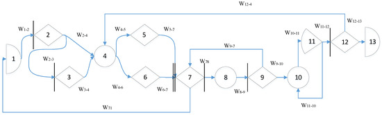
Figure 3.
GERT-diagram of the software development process.
The model is considered as a directed probabilistic graph G = (V,E) with a set of nodes V = {1,…,13} and a set of arcs E ⊆ V × V. Each arc Wij specifies the probability of passing pij and the duration (or cost) distribution Tij. For decision nodes, the sum of the probabilities of the output arcs is equal to one. Node 7 has input logic I-AND (triggered only after receiving results from nodes 5 and 6), and the output logic in all decision nodes is O-OR.
The process starts at node 1 (Project concept) and, with a mandatory transition, W12 moves to node 2, where a decision is made on the need for an AI requirements assistant. If the option “Yes” is selected, node 3 (AI Requirements Assistant) is executed with a transition W34 to the specification. In this step, the assistant structures the informal requirements of stakeholders into requirements artifacts (user stories, acceptance criteria, non-functional constraints), eliminates contradictions, and forms traceability traces.
It should be noted that this transition models a conscious choice to use the AI Requirements Assistant module as a preliminary stage of formalization. Semantically, this is the probabilistic output of the decision node 2. p2−3 is normalized together with p24 (p23 + p24 = 1) and calibrated by design factors (degree of unstructuredness of the elicitation input materials, novelty of the subject area, multilinguality of the sources, pronounced security restrictions, maturity of the team). The time costs of the transition itself are considered negligibly small (decision), and the main duration is taken into account at the next stage of processing (node 3). Selecting the W23 branch activates the AI assistance procedures, normalization and deduplication of stakeholder statements, detection and resolution of contradictions, extraction of entities and relationships (glossary, NFR classification), generation of user stories and acceptance criteria, and construction of the initial traceability matrix. The result is an agreed package of requirements artifacts, which is then transmitted by the W34 arc to node 4. Empirically, its application reduces the expected value of E[T3−4] and subsequent returns at later stages (in particular, p9−7 and p12−4, which affects the total cycle time and the probability of reaching the terminal node 13.
If the option is “No”, W2−4 is activated, and the process bypasses node 3, moving directly to node 4 (Functional specification). Node 4 consolidates the requirements into a single document that serves as the source of truth for the following stages.
From the specification, the branching occurs in parallel, arcs W45 and W46, respectively, trigger node 5 (System design blueprint), where the architecture, module interfaces, data model, and security aspects are processed, and node 6 (Interface and UX model), where interaction flows and user interface prototypes are designed. Both flows must be completed, after which their results converge in node 7 (Successful Collaborative assessment). This is a synchronous node with input logic I-AND; it is triggered only if artifacts 5 and 6 are present.
To make the implicit-AND (I-AND) join and feedback reduction concrete for readers unfamiliar with GERT, we include a short pseudocode recipe that reduces a minimal subnetwork with one feedback loop and a parallel I-AND join. The recipe works at the level of the first two moments (mean and variance) and is fully consistent with the semantics introduced above.
- function GeometricLoopReduce(mu, var, p):
- # total time until first success (geometric number of attempts)
- mu_eq = mu/p
- var_eq = var/p + (1 − p)/(p^2) * (mu^2)
- return mu_eq, var_eq
- # Main reduction: parallel I-AND with one feedback loop on A
- # Inputs: mu_A, var_A, p_A, mu_B, var_B, rho # set rho = 0 if unknown
- function IAND_Reduce(mu_A, var_A, p_A, mu_B, var_B, rho = 0):
- (mu_A_eq, var_A_eq) = GeometricLoopReduce(mu_A, var_A, p_A)
- # If branch B also has a loop, replace with:
- # (mu_B_eq, var_B_eq) = GeometricLoopReduce(mu_B, var_B, p_B)
- mu_B_eq = mu_B
- var_B_eq = var_B
- # Conservative I-AND (serialized upper-bound): sum of branch equivalents
- mu_AND = mu_A_eq + mu_B_eq
- sd_Aeq = sqrt(var_A_eq)
- sd_Beq = sqrt(var_B_eq)
- var_AND = var_A_eq + var_B_eq + 2 * rho * sd_Aeq * sd_Beq
- return mu_AND, var_AND
Node 7 performs a joint (engineering-product) assessment of the architecture and UX alignment with the requirements. A typical output from this node is arc W7−8 to automated checks. Another possible output is arc W7−1, which models a strategic “pivot” (return to rethinking the concept in case of fundamental inconsistencies).
Next, node 8 (automated checks: AI static analysis + CI/CD build and unit tests) is executed. This is the operational stage where AI-supported static analysis (AI static analysis) complements classic checks; dependencies and security policies are analyzed, anti-patterns and potential defects are detected, a build is performed in the CI/CD pipeline, and unit tests are run.
Node 8 acts as a “quality filter” before human review at node 9. The input is code and configuration changes, dependency manifests, infrastructure as code descriptions, and build telemetry, and the output is a machine-readable package of test results with risk ranking, problem localization, and short fix suggestions, as well as assembled artifacts with unit test results. A key component is AI-supported static analysis, which complements classic SAST with semantic interpretation of call contexts (LLM/ML models), code graph analysis (code property graph, taint-propagation), dependency and SBOM checks for known vulnerabilities and license incompatibilities, search for secrets and configuration flaws, and revision of IaC manifests. The results are aggregated into a vector of quality indicators SAI = (Ssec, Srel, Sperf, Slic, Sconf), which is then combined with the assembly and unit test metrics to form a “quality gate”. Formally, the passage to node 9 can be written as the condition
where —a set of build metrics (success, coverage, stability),
τ—threshold configurable by quality policies.
The influence of node 8 on the network parameters is manifested both in the time distributions and in the subsequent probabilistic choices. First, the expected duration of preparation and execution of checks decreases with increasing quality of static analysis, which is conveniently modeled by the dependence
where is —component SAI, which reflects the overall “cleanliness” of the code based on the results of AI analysis.
For dispersion, exponential reduction is natural.
where is —weighted combination of quality components.
Second, improving security, reliability, and performance reduces the likelihood of rejection during review. Easily enter risk indicators
and describe the rollback as a logistic function
so that the reduction in risk components induced by node 8 monotonically reduces p9−7 and shortens the local cycle 7 → 8 → 9 → 7.
The indirect effect is also observed in the integration loop, removing system defects before entering node 10 statistically reduces the probability of repeated deployments and retests p11−10, which can be modeled by a similar logistic relationship with a different set of coefficients.
From the point of view of parameter identification, it is advisable to store the telemetry of node 8 (types and severity of findings, confidence level, applied corrections, time costs) and use it to calibrate α, ν, β, and the shapes of the T78, T89 distributions on historical iterations. In practice, this is implemented as a logistic regression for p9−7 with stabilization (for example, isotonic calibration) and Bayesian update of the duration parameters. In this form, node 8 not only “fixes” defects, but also quantifies their impact on the network trajectories; it reduces E[T78] and Var(T78), corrects p9−7 and, indirectly, p11−10, increasing the chances of reaching the terminal node 13 within the given time budgets.
The results of this step are transmitted by arc W89 to node 9 (Peer verification), where one of the decisions is adopted based on the results of the expert review. In case of success, the transition from W9−10 to the integration deployment is approved. In case of problems, the return of W9−7 to the stage after merging the artifacts is approved (which forms a local cycle of “revision → auto-checks → review”).
Integration deployment is performed in node 10 (Integration environment deployment) with subsequent transition W10−11 to node 11 (Automated tests + Quality validation), where regression, load, and other automated tests are launched and a consolidated quality validation is performed. If the tests are passed, the arc W11−12 is activated for final acceptance. If discrepancies are detected, arc W11−10 is activated, forming an internal loop of retests and redeployments until a given quality level is achieved.
Final acceptance is implemented in node 12 (PO/Stakeholder review). If the decision is positive, the transition W12−13 to the terminal node 13 (Increment delivery) is performed, which corresponds to the delivery of the increment. If the scenario is negative, the arc W12−4 is activated, which starts the refinement macrocycle. The flow returns to specification refinement (node 4), then again passes through stages 5 and 6, their combination in 7, automatic checks in 8, review in 9, integration 10−11, and re-acceptance in 12. Thus, the network contains three characteristic feedback loops: local 7 → 8 → 9 → 7 (refinements based on the review results), integration 10↔11 (retest/redeployment), and macrocycle 12 → 4 → ⋯ → 12 refinement based on the acceptance results. The rare but costly W71 arc formalizes the “pivot” scenario.
The final interpretation is as follows. Two AI nodes are explicitly built into the process topology—node 3 (AI Requirements Assistant) as an optional branch of early requirements formalization (driven by the decision in node 2 and leading to W34, and node 8 (AI static analysis as part of automatic checks) as a mandatory operational stage before the review. The remaining nodes and arcs retain the basic semantics of the engineering circuit. The probabilities pij in the decision nodes are normalized to 1 (in particular, p23 + p24 = 1, p9−10 + p9−7 = 1, p11−12 + p11−10 = 1, p12−13 + p12−4 = 1), and the distributions Tij are set according to the practical data of the project. This description format makes the role of AI transparent. In this case, nodes 3 and 8 affect both the probability of reaching node 13 and the expected iteration duration.
According to the GERT diagram shown in Figure 3, the equivalent W-function of software development time can be represented as a composition of two interconnected process components. Due to the high analytical complexity of formalizing the full model, we will decompose the diagram into two components: (1) “Software Design” and (2) “Code Implementation and Testing”. The relationship between the components (feedback 7 → 1 and 12 → 4) is expedient to formalize by means of a fuzzy GERT model, where the fuzzy parameterization of probabilities and durations reflects epistemic uncertainty.
For each arc (i, j), we define the W-function as the product of the probability weight coefficient and the Laplace transform of the duration distribution:
where the durations are assumed to be gamma-distributed (k,) (positive random variables with wide variability, suitable for “times between events”). This choice agrees well with the “random walk” analogy for human communication and creative steps in design. The final duration is the sum of many stochastic steps, which is naturally approximated by the gamma law.
Consider the first component of the “Software Design” model (nodes 1–7). In our model, this stage includes: 1 → 2 (initial solution), an optional branch 2 → 3 → 4 with AI Requirements Assistant, a direct transition 2 → 4 (if AI is rejected), parallel design 4 → 5 and 4 → 6, and a synchronization node 7 (Successful Collaborative assessment) with I-AND logic at the input.
The main parameters of transitions at the “Software Design” stage are presented in Table 2.
Table 2.
Characteristics of transitions at the “Software Design” stage.
Let us denote the “direct” (without taking into account the cycle 7 → 1) transition 1 → 7 as
For AND-merge (4 → {5,6} → 7), we apply analytically closed serialized approximation (pessimistic estimate of synchronization time):
In the real process, the completion time of the parallel design branches is determined by the last finishing path. Formally, letting and , the synchronization time is
To retain a single closed-form W-function for the whole network, we adopt a conservative serialized surrogate
which upper-bounds and avoids optimistic bias in deadline-related metrics at the price of overestimation. This choice preserves the analytic tractability of Equations (7)–(19) and provides a safe planning estimate. Alternative treatments (moment-matching for max, hybrid analytic-simulation) are left for future extensions.
Then, taking into account the return loop “pivot” 7 → 1, the equivalent transfer function of the first component has the form of a geometric reduction:
Let us consider the second component of the model, “Code Implementation and Testing” (nodes 7–13).
The stage includes automated checks with AI static analysis (7 → 8), peer-review (8 → 9), local refinement cycle 9↔7, integration deployment 10 and retest cycle 11↔10, as well as final acceptance 12 and release 13. The feedback 12 → 4 is inter-component and is further used to build a “reinforced” (fuzzy) model of the entire network.
The main parameters of the transitions at the stage “Code implementation and testing” are presented in Table 3.
Table 3.
Characteristics of transitions at the “Code Implementation and Testing” stage.
In this example, serial connection with local loop reduction gives:
The first part of expression (10) formalizes the reduction in the cycle 9↔7. The second part of expression (10) describes the reduction in the cycle 11↔10.
A complete system is formed by a series connection and with inter-component feedback 12 → 4. For 12 → 4 we apply fuzzy probabilities and/or vague durations (triangular or trapezoidal numbers), advancing them through (1)–(5) according to the Zade expansion principle [27,28,29].
The numerical inversion of the Laplace transform provides an estimate of the system’s time metrics. As a result, the decomposition allows us to obtain interpreted partial equivalent W-functions (9) and (10), and the “enhanced” GERT model allows us to combine them into a holistic characteristic function of the iteration time, taking into account the uncertainties of the requirements, design, and acceptance procedures.
Let us expand the components of expressions (7)–(10) and reduce the model to a closed equivalent W-function of the entire network. To do this, we substitute these components into the aggregated transfer functions of the components.
Lets start with the first component, “Software Design”. We will explicitly rewrite the aggregate “initial” transition 1 → 4, taking into account the optional branch of the AI assistant (2 → 3 → 4).
According to the definition P(s) (11) we have
Therefore, taking into account (6),
where p2−3 + p2−4 = 1.
Next, for the parallel branches 4 → 5 → 7 and 4 → 6 → 7, we adopt a serialized approximation of AND-merge as (8):
The serialized form (13) is deliberately conservative. Using this expression, the product of Laplace transforms for two consecutive branches, the synchronization time is formalized. Thereby overestimating the duration relative to the approximate maximum of the two stochastic paths. This choice reduces the risk of optimistic planning errors. If necessary, formal accuracy can be easily improved by moment matching for Tmax and numerical inversion. However, for analytical transparency and further inferences, this is not required. Semantically (13) formalizes the achievement of the 7th checkpoint in the presence of both finished artifacts. And it is they who determine the time profile of the final design stage.
Taking into account the pivot loop 7 → 1, the effective transition 4 → 7 is reduced by a geometric factor, we rewrite (9) in expanded form:
The geometric reduction in the denominator of expression 14 has a transparent engineering meaning. multiplier is equal to the “amplification factor” of the large return to zero. While the convergence condition < 1 guarantees that the expected number of such returns is finite. Thus, even with rare strategic revisions to the concept, the process on average moves forward and does not turn into an endless wandering.
Lets examine the second component, “Code Implementation and Testing.” Here, according to expression (10), we have a sequence with two local loops. Their explicit reductions are given as follows:
where each according to (6), and the probabilities at the decision nodes are normalized: p9−10 + p9−7 = 1, p11−12 + p11−10 = 1. The sequential transfer from 7 to 12 is equal to B(s) = B1(s)B2(s).
Both reductions have the same structure. The numerator formalizes the “direct” sequential movement, while the denominator is a geometric correction for the expected number of repetitions. At zero, the convergence conditions simplify to , which in a real process is performed automatically since (otherwise the team would never achieve through the review and integration tests). Here you can see the direct path of influence of node 8 (AI static analysis). decrease by , partially, “compression” of arc lengths 7 → 8 and 8 → 9 lead to a decrease in the denominator in (14), i.e., they reduce the average number and “cost” of review cycle repetitions.
At the output 12 of the node, we have an alternative. Output 12 → 13 and intercomponent return 12 → 4.
Based on this, we can formalize the following.
Next, it is convenient to introduce an “open” transmission from 4 to 12 through 7, which already takes into account the pivot loop and both local reductions:
Closing the intercomponent feedback 12 → 4 with the “loop gain” Fss gives the final equivalent W-function of the entire network (from 1 to 13):
Size sets the importance of acceptance. The larger it is, the less often the command returns to specification, and the smaller the contribution of the second denominator in (19). At the same time, the parameters fix the “price” of such a return. The more complex the requirements refinements and design redesign, the “heavier” the contribution of F(s) to the overall transfer becomes [30].
Since is the Laplace transform of the corresponding time measure, standard operations allow you to directly obtain key indicators.
The probability of completing the iteration (reaching node 13) is equal to the value at zero:
Value of equals the probability of completing an iteration. A useful indicator in cases where the model allows for absorbing failure modes (in particular, a potentially infinite cycle of strategic reversals is fundamentally possible). The derivatives at zero give the conditional expectation and variance of the calendar duration of the iteration, in this sense, the geometric multipliers in (13), (14), (15), and (19), formalize the increase in the mean values, which is proportional to the expected number of repetitions of the corresponding cycle. At a practical level, this means that if, say, p9−7 is reduced by 10%, then to first approximation the average number of review cycles falls by about the same amount, and the contribution of B1(s) in (19) proportionally reduces the expected iteration time.
Under the termination condition, the expectation and variance of the iteration time are expressed in terms of derivatives at zero:
From a practical point of view, all parameters (11)–(19) identified from process telemetry. For P(s) and A(s) identified from elicitation and design data (including the AI Requirements Assistant branch). For B1(s) calculated from AI static analysis and CI/CD metrics, as well as review results. For B2(s) identified from integration tests. For S(s) and F(s) generated from acceptance statistics.
If the intercomponent transition 12 → 4 carries significant epistemic uncertainty, the application of fuzzy parameterization , is consistent with the already adopted scheme. Relevant -functions are simply substituted into (17) and passed through expressions (18) and (19) according to the Zadeh expansion principle, after which the numerical inversion of the Laplace transform provides estimates of the time metrics with confidence intervals. Thus, expressions (11)–(21) complete the formalization of the model and are ready for the substitution of data for a specific project.
Given the practical conditions of project implementation, the full model should reflect not only the random (actually stochastic) variability of work durations, which is already taken into account through gamma distributions in the W-functions of arcs, but also the epistemic uncertainty of parameters, caused by incomplete knowledge at the early stages, domain novelty, and variability of the organizational context. That is why it is advisable to specify some of the network parameters, for example, the transition probabilities pi−j and the time parameters (ki−j,θi−j) of critical arcs (in particular 2 → 3, 7 → 1, 12 → 4, as well as those that determine the quality gate after node 8), as fuzzy numbers of type-1. In this case, the corresponding W-functions take the form
The final transfer function of the network preserves the fractional-rational structure (19), but with fuzzy parameters. The estimation is performed according to the principle of Zade expansion through α. For each parameters , , are replaced by interval estimates, and expression (19) is calculated intervalically, which generates a range of values
At the point s = 0, this gives a fuzzy probability of the iteration ending. In particular,
Derivatives are used for time points and at zero (while preserving the monotonicity of the corresponding mappings), which provides interval estimates and . Thus, the model returns not point, but interval (or, in fuzzy mathematics terms, possibility-necessity) characteristics of key metrics, and the narrowing of α-intersections in the process of CI/CD telemetry accumulation, review, and acceptance reflects the gradual reduction in epistemic uncertainty without changing the structure of the GERT composition.
Thus, the mathematical model (11)–(19) not only specifies the equivalent W-function of the network but also makes transparent the mechanism of influence of local solutions and quality of artifacts on global time indicators. Together with (21) and (22), it forms a self-sufficient tool for forecasting terms and risks, where the parameters are directly related to the measured process quantities, and the two AI-insertions (nodes 3 and 8) have an explicit and reproducible effect on the structural elements of the transfer function.
A mathematical model of the software development process with elements of hybrid management has been developed. Unlike others, the model takes into account the topology of the real hybrid project management process and provides causal levers (loop/duration parameters). This allows for the return of interval metrics under uncertainty and is directly translated into planning indicators.
2.4. Telemetry-to-Parameter Calibration
To ensure transparency and reproducibility, we detail a step-by-step workflow that transforms raw software-process telemetry into quantitative parameters of the GERT network: branch probabilities and arc-duration distributions .
In brief, the calibration pipeline executes:
- −
- Extract and harmonize logs
- −
- Clean and window by iteration, apply interquartile-range (IQR) and median absolute deviation (MAD) rules, and join entities by {iteration_id, issue_key, PR_id, build_id, commit_SHA}
- −
- Map events to GERT arcs (Section 2.3) and compute per-arc durations ()
- −
- Estimate branch probabilities with beta–binomial smoothing (Jeffrey’s prior), with a logistic + isotonic calibration for
- −
- Fit Gamma durations via the method of moments with 95% bootstrap CIs
- −
- Export calibrated parameters to CSV and simulator inputs, with QA checks (probabilities sum to one at each split; durations are non-negative)
Requirements traceability (user stories/epics, acceptance criteria, trace matrix linking requirements to commits/pull requests, approval status)
Peer review (pull/merge-request identifier, review decisions approve/request-changes, diff size, number of review rounds)
CI/CD (Continuous Integration/Continuous Delivery) builds and tests (build ID, commit SHA, build time, unit/regression/load test statuses, coverage, flaky-test rate)
SAST (Static Application Security Testing) and policy checks (issue counts by severity, SBOM (Software Bill of Materials), and license findings, secret/configuration flags)
Acceptance/PO (Product Owner) decisions (accept/return and return reasons)
Cleaning and joining. We de-duplicate events, window them by iterations (e.g., sprint/iteration IDs), document missing data rules, and suppress obvious outliers using IQR/MAD with audit flags. Each event is then mapped to GERT arcs defined in Section 2.3:
- −
- review and the review branch ;
- −
- integration/re-test ;
- −
- acceptance
- −
- joint-assessment “pivot” ;
- −
- requirement-assistant branch .
For arcs , , , , we compute empirical proportions over the iteration window and apply beta-binomial smoothing with the Jeffreys prior for small-sample stability:
For the review return branch we further incorporate a telemetry-based risk vector xxx from automated checks (see Section 2.3, Equations (4) and (5)):
We fit a logistic model, logit on historical iterations and apply isotonic calibration to correct the probability scale. The calibrated is then plugged into Equations (4) and (5), keeping causal consistency with node 8 (AI-augmented static analysis).
For each arc , the duration is measured as the timestamp difference between stage start and completion (e.g., (): “start automated checks/build”–“ready for review”). Assuming the Gamma law as in Section 2.3, we estimate parameters by the method of moments:
where are sample variance/mean after cleaning; 95% confidence intervals are obtained via bootstrap (B = 1000).
Illustrative telemetry-based calibration is presented in Table 4.
Table 4.
Illustrative telemetry-based calibration (micro-case: 4 iterations).
2.5. Scenario Parameters and Reproducibility Settings
To ensure transparency and repeatability, this subsection lists the exact numeric inputs used to produce the results for both scenarios (“No-AI” and “AI-enabled”) and the corresponding computational settings. While Table 1 and Table 2 define the model structure, Table 5 and Table 6 enumerate, respectively, the transition probabilities , and duration parameters per arc that were used in the simulations. All results in Section 3 were generated with a discrete-event Monte–Carlo simulator using N = 300,000 iterations per scenario, a fixed random seed (1729), and kernel density estimation (KDE) with Silverman’s rule [31] applied to normalized histograms.
Table 5.
Transition probabilities used in simulations (No-AI vs. AI-enabled).
Table 6.
Gamma duration parameters used in simulations (No-AI vs. AI-enabled).
In addition to the base runs (N = 300,000, fixed seed 1729, KDE via Silverman’s rule), we perform systematic robustness checks:
- −
- ±10% parameter perturbations of transition probabilities and arc-duration scales (probabilities are renormalized at each node)
- −
- Alternative duration laws by replacing Gamma with Weibull distributions, moment-matched to each arc’s mean and variance
- −
- Dependency relaxations by inducing moderate positive correlation among related stages via a Gaussian-copula (target within design, verification, and acceptance groups)
- −
- Fuzzy membership variations, reweighting expert weights by ±25% followed by renormalization and centroid defuzzification
For all settings, we report 95% bootstrap confidence intervals (B = 1000 resamples) for the median, , , at and for-loop PMFs at zero counts
A minimal, fully reproducible package (synthetic/anonymized telemetry schema, scenario parameter tables with fuzzy intervals, and all simulation/plotting scripts with a fixed random seed of 1729) is publicly available at https://github.com/serhsemenov/artykl (accessed on 28 October 2025). The repository contains a step-by-step README and scripts to regenerate all Section 3 figures and the unified summary table.
Parameterization follows standard practice: positive task times are modeled with Gamma laws. Shape values encode multi-step activities with moderate variability, while AI speed-ups are implemented by scaling the scale parameter θ\thetaθ (preserving phase structure and interpretability). Scenario deltas target the loops most affected by AI support—post-analysis rework , redeploy/retest , and acceptance rework reflecting fewer returns and faster fixes with an AI requirements assistant (node 3) and static analysis (node 8). This combination yields the observed left-shift and narrowing of iteration-time distributions (Figure 4, Figure 5, Figure 6, Figure 7, Figure 8, Figure 9, Figure 10, Figure 11 and Figure 12) and increases the share of iterations without loops (Figure 13, Figure 14, Figure 15 and Figure 16).
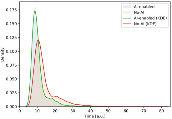
Figure 4.
Empirical probability density of total iteration time for the “AI-enabled” and “No-AI” scenarios (as indicated in the legend), estimated from 300k Monte–Carlo iterations. The AI-enabled curve is visibly left-shifted and slightly narrower, indicating shorter typical durations and reduced dispersion—supporting higher on-time release chances in Section 3.
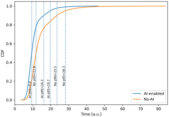
Figure 5.
Cumulative distribution functions (CDF) of total iteration time (300k Monte–Carlo iterations). The AI-enabled CDF first-order stochastically dominates the baseline: for any deadline is higher under AI, implying earlier completion across thresholds.
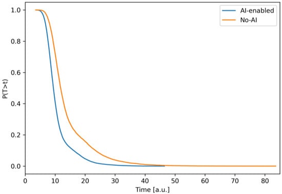
Figure 6.
Survival (reliability) functions for total iteration time. Lower survival under AI across T > t means fewer long overruns and a smaller tail risk versus the baseline.
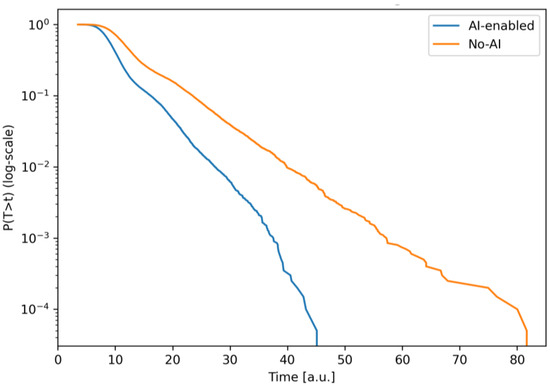
Figure 7.
Survival functions on a logarithmic scale. Log-scale reveals extreme-delay probabilities; the AI-enabled curve remains uniformly below the baseline, highlighting materially lower tail risk for rare but costly overruns.
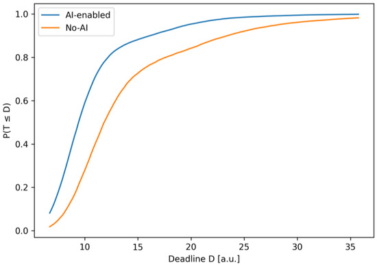
Figure 8.
Deadline-achievement curves . The AI scenario achieves a higher probability of meeting deadlines for the full range of D; the gap is largest near typical iteration lengths, directly improving release reliability.
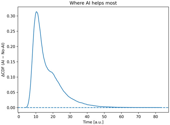
Figure 9.
Difference in Cdfs, . Positive indicates uplift due to AI. The curve pinpoints where AI brings the largest on-time benefit and where gains taper off.
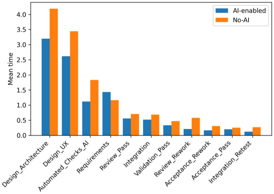
Figure 10.
Average contributions of stages to the total iteration time (top stages).
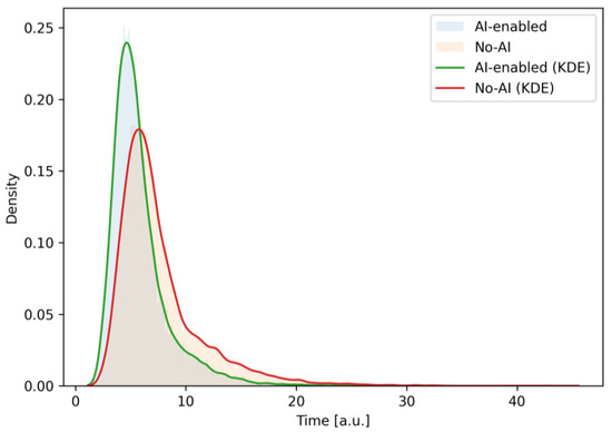
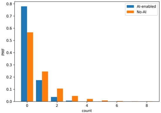
Figure 13.
Empirical probability mass function (PMF) of review–rework cycles per iteration (loop 9 ↔ 7). AI shows a substantially higher mass at zero cycles and lower probabilities for multiple cycles, indicating fewer post-review returns and faster stabilization.
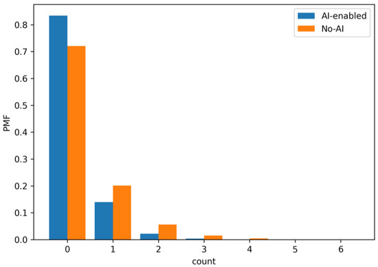
Figure 14.
PMF of integration retests per iteration (loop 11 ↔ 10). Under AI, the probability of zero retests increases and the tail for multiple retests shrinks, implying smoother integration and reduced re-verification load.
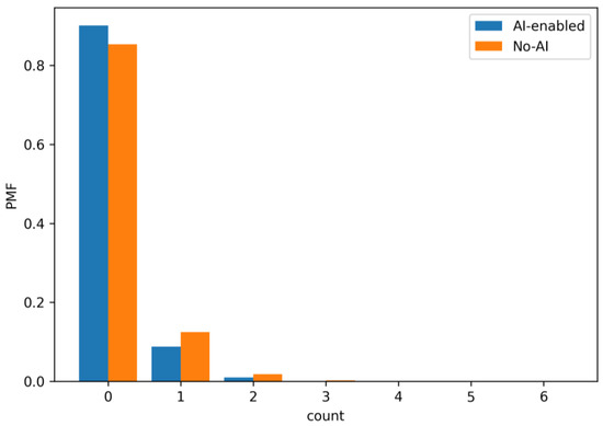
Figure 15.
PMF of acceptance returns per iteration (arc 12 → 4). AI reduces the probability of any return and compresses the right tail, signaling fewer late-stage changes and more first-pass acceptances.
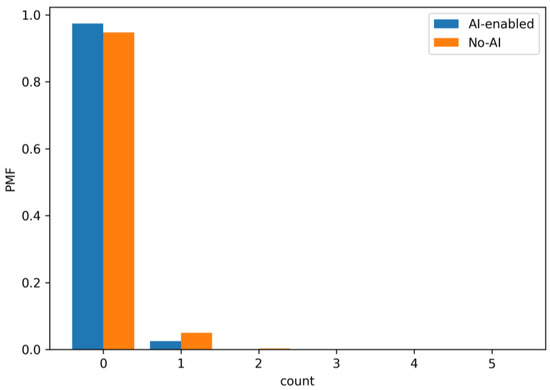
Figure 16.
PMF of radical concept revisions per iteration. The AI scenario concentrates probability at lower counts, indicating that upstream assistance limits major rework.
All analyses and simulations were run in Python 3.11. Monte–Carlo sampling and closed-form routines used NumPy/SciPy; data handling used pandas; bootstrap confidence intervals relied on NumPy resampling; figures were produced with Matplotlib 3.10.7; notebooks were executed in Jupyter 4.4.10. Source code and environment files (e.g., requirements.txt) are provided in the repository (Supplementary Materials), with random seeds and commit hashes recorded for reproducibility.
All computations were performed on a standard x86-64 workstation (8 logical cores, 16 GB RAM, 512 GB SSD). The code is CPU-only (no GPU required) and is portable to Windows 10/11 and macOS.
3. Results
For both scenarios, all numeric parameters used in the simulations are provided in Table 3 and Table 4 (probabilities and Gamma parameters).
The developed and described mathematical model provides analytical transparency. However, due to the complexity of the composition and the presence of uncertainty, it requires numerical verification and quantitative illustration. We will conduct an empirical study of the behavior of the model. To do this, we will check the expected shift in the Distributions towards shorter iterations, the localization of the zones of the greatest impact from AI-insertions, and analyze the contribution of individual delay mechanisms.
We will conduct further analysis for the two process configurations. The first is AI-enabled (node 3 “AI Requirements Assistant” is activated by the decision in node 2; node 8 contains “AI static analysis”). The second scenario assumes that the AI elements are ignored (branch 2 → 3 is blocked; node 8 operates without AI-boosting).
While the network’s closed-form W-function (Section 2.3) provides structural insight and moments (termination probability, mean/variance of the iteration time, expected number of loops), the detailed iteration-time distributions and all distributional plots in this section are obtained via a discrete-event Monte–Carlo simulator built from the GERT topology and the parameters of Table 1 (including the serialized upper-bound at the I-AND merge, see Section 2.3). We do not numerically invert Equation (19) for the figures. Analytics are used for tractable invariants, simulation, and for full distributions.
For both scenarios, the transition probabilities and the parameters of the gamma distributions of the arcs correspond to Table 1 and Table 2. The epistemic uncertainty of the critical parameters (primarily 7 → 1 and 12 → 4) is interpreted as fuzzy intervals and, where necessary, is passed through formulas (17)–(19) according to the Zadeh expansion principle [27,28,29]. The basic treatment of I-AND at node seven is performed in a “serialized” conservative approximation (Formula (13)), which is consistent with the analytical conclusions.
3.1. Methodological Baselines and Unified Summary
To position our framework against established paradigms, Table 7 contrasts core capabilities of Petri nets/GSPN, fuzzy-PERT, discrete-event simulation (DES), and our GERT with fuzzy parameterization. We use identical workflow semantics (branching, feedback, I-AND mergers) for comparison of modeling affordances rather than claiming numerical parity across toolchains. We also provide a unified quantitative summary of our two scenarios in Table 8 (median, at the maximum gap, loop PMFs), reported with 95% bootstrap confidence intervals for transparency.
Table 7.
Capability baseline across modeling paradigms (qualitative comparison).
Table 8.
Unified scenario summary (median, , rework PMF; values with 95% bootstrap CIs; Δ = AI − No-AI, relative % in parentheses).
Table 8 consolidates the quantitative contrast between the two scenarios. On location metrics, the AI-enabled configuration reduces the median iteration time from ≈11.9 to ≈9.4 (about −21%) and compresses the upper tail: drops from ≈23.5 to ≈16.1 (−31%), and from ≈28.2 to ≈19.7 (−30%). These shifts indicate not only faster typical iterations but also materially fewer long overruns, which drives planning reliability.
On deadline reliability, the probability of finishing by a representative short deadline increases from ≈0.45 to ≈0.76 (+0.31), and by a more relaxed deadline from ≈0.78 to ≈0.96 (+0.18). The maximum uplift of the CDF (the largest pointwise advantage in on-time probability), , is ≈0.31 occurring around − pinpointing where AI support yields the strongest schedule benefit.
Loop statistics corroborate these gains. For the review–rework loop () the probability of zero cycles rises from 0.56 to 0.77 (+21 percentage points), with mass shifting away from one and multiple cycles; the expected number of cycles decreases accordingly. For integration retests (11↔10), the chance of proceeding without retest increases from 0.72 to 0.84 (+12 pp), and the tail of multiple retests shrinks. At acceptance (), the probability of any return drops from 0.15 to 0.10 (−5 pp), implying fewer late-stage changes and smoother finalization. Taken together, these loop PMFs explain the global left-shift and tail compression in the total-time distributions.
3.2. Distributional Characterization and Deadline Reliability
For each scenario (“AI” and “No-AI”), we simulate N = 300,000 independent iterations with a fixed random seed. Imooth curves are kernel density estimates (Silverman’s rule [31]) over normalized histograms. Unless noted otherwise, Figure 4, Figure 5, Figure 6, Figure 7, Figure 8, Figure 9, Figure 10, Figure 11, Figure 12, Figure 13, Figure 14, Figure 15 and Figure 16 reflect these empirical distributions; analytical values from Section 2.3 (e.g., , mean/variance, loop-related terms) are reported in-text for reference.
Because the serialized surrogate upper-bounds the true synchronization time almost surely, all location metrics shift conservatively: for any . For the mean, the bias admits an exact identity
hence , where and . For gamma-distributed arc durations with parameters , the arc means are , so and . This identity quantifies the conservative shift at the mean level exactly and explains why the surrogate is most pessimistic when the two branches have comparable meanings.
Figure 4 shows the probability density graphs of the total iteration time for scenarios with and without the use of AI.
In this figure, the smooth curves are obtained using the Kernel Density Estimation (KDE, Silverman rule) method, and the histograms are shown only as a background for visual control of the normalization.
As can be seen from the figure, there is a clear leftward shift in the distribution in the scenario with the use of AI (modal zone ~8–9 conventional time units) relative to the scenario without its use (≈10–12), as well as a smaller dispersion and a thinner right tail. This indicates a reduction in both typical execution time and the risk of long delays due to AI insertions at the requirements formalization (node 3) and automatic checks (node 8) stages. The slight “shoulder-like” shape of the red curve in the range of ~18–25 corresponds to additional cycles of reviews and retests (loops 97 and 11 ↔ 10), the intensity of which decreases when using AI.
Figure 5 shows the graphs of the iteration duration distribution function (CDF) for scenarios with and without the use of AI.
The graph compares the empirical CDFs of the total iteration time. The AI-enabled curve is located further to the left over the entire range of t, reflecting first-order stochastic dominance. For any fixed time, the probability of completing the iteration no later than t is higher when using AI. Dotted vertical lines indicate percentiles for the AI scenario. (p50–mediany of 50% iteration time p50 ≈ 9.4), (p90–90th percentile at 90% iteration time p90 ≈ 16.1), (p95–The 95th percentile at 95% of iteration time p95 ≈ 19.7). Without the use of AI, p50 ≈ 11.9, p90 ≈ 23.5, p95 ≈ 28.2. The left shift and greater steepness of the curve, for the example of using AI mean both a shorter typical time and lower variability. In practice, this is interpreted as an increase in the probability of meeting work deadlines and a significant reduction in “long” iterations that form schedule risks.
Figure 6 shows graphs of the reliability function (survival) of the total iteration time S(t) = P(T > t) for scenarios with and without the use of AI.
The graph shows the probability of exceeding a given threshold time t in one iteration, i.e., S(t) = 1 − F(t). In both configurations, S(t) is monotonically decreasing, but the AI-enabled curve falls significantly faster and lies lower over the entire range of t.
This means that for any fixed threshold, the risk of “not meeting” the time with AI is lower. The most noticeable difference is observed in the area of working durations (~8–25 a.u.). At these values, the probability of exceeding in the scenario with AI is 1.5–3 times lower, while the “tail” without AI persists up to much higher t. The resulting picture is consistent with the CDF (Figure 5) and quantitatively reflects the reduction in the risk of delays due to AI-insertions in nodes 3 and 8.
Figure 7 shows graphs of the reliability function (survival) of the total iteration time S(t) = P(T > t) for scenarios with and without the use of AI, but on a logarithmic scale.
The logarithmic scale on the y-axis highlights rare, extreme delays, which are critical for effective release planning. Both curves fall monotonically, but for scenarios with AI, a sharp “tail clipping” is observed. Already in the interval t ≈ 35–45, the probability of exceeding drops to levels of 10−3–10−4, while in the scenario without AI, the order of 10−2 is maintained at the same points. Therefore, in the zone of large t, the risk of delays with AI is lower by 1–2 orders of magnitude. In fact, the “tail” of the distribution with AI ends around t ≈ 40–45, while without AI it extends to t ≈ 70–80. Almost straight sections in the log-scale indicate an approach to exponential behavior (phase-exponential mixture), while the lower slope of the AI curve corresponds to a lower intensity of large delays. Thus, AI not only reduces typical time (see Figure 4 and Figure 5) but also reduces the likelihood of extreme delays, which is critical for effective release planning.
Figure 8 shows the deadline achievement curves P(T ≤ D) for scenarios with and without the use of AI.
The dependence of the probability of completing an iteration no later than the given deadline D (i.e., F(D)) for two process configurations is shown. The curve of the scenario using AI lies higher over the entire range of D values, which means a greater chance of successfully meeting the deadline for any realistic deadline. In particular, at a service level of 0.9, the corresponding deadlines correspond to the 90th percentile of the CDF (see Figure 5). The scenario using AI requires D ≈ 16.1 a.o., while the scenario without using AI requires about 23.5a.o. Thus, the use of AI reduces the necessary time margin to achieve a given schedule reliability and at the same time reduces the risk of delay at a fixed D. The quasi-sigmoidal shape of the curves reflects a rapid increase in the probability in the region of typical durations and further saturation at large D.
Figure 9 shows the difference in the cumulative distribution functions which is interpreted as a point increase in the probability of completing the iteration by time t due to AI.
The curve reflects the pointwise increase in the probability of completing an iteration no later than time t in the scenario with AI compared to the scenario without it. Over the entire range, ΔF(t) ≥ 0, which empirically confirms the first-order stochastic dominance of the configuration with AI. The maximum is reached near t ≈ 10 − 12a.o. time, where ΔF is about 0.30–0.32, i.e., the probability of completing the task on time with AI is ≈30 percentage points higher. Then the increase monotonically decreases and approaches zero in the far “tails”, where both scenarios rarely last that long. So, the greatest return from AI is observed in the area of typical durations, and it is there that the chance of meeting practical deadlines increases the most. In the “tail,” the advantage decreases, which is consistent with the reduction in the frequency of review loops and retests.
Figure 10 presents the average contributions of stages to the total iteration time (top stages). The bars in this figure reflect the estimates
for the main stages of the process (according to Monte–Carlo results) [30]. In this case, is the time spent on stage k in the nth trajectory. A comparison is shown for configurations with and without the use of AI.
The dominant contribution to the total duration is made by design (architecture and UX). With AI, both components shift down by about a quarter (approximately −20…25%), which is consistent with better early requirements processing (node 3) and the coordinating I-AND-join at node 7.
The Automated checks (incl. AI static) stage is also noticeably reduced (≈−20…30%), which corresponds to the effect of AI-supported static analysis at node 8. The Requirements stage sees a reduction in about a third of the time (≈−30…40%), reflecting the benefit of the AI assistant during requirements structuring and tracing.
The largest relative changes are characteristic of rework: “Review–Rework”, “Integration_Retest”, and “Acceptance_Rework” are significantly reduced by 2–3 times (with point reductions in ≈50–70%), which is consistent with the PMF of discrete loops in the subsequent figures. At the same time, Review Pass in the scenario with AI is somewhat longer, which is the expected compensatory effect. Part of the mass goes from “rework” to “pass”, and the total review time (pass + rework) remains no larger and is accompanied by a decrease in the number of iterations. Taken together, the graph shows where exactly the left shift in CDF/Survival for the total time comes from. Due to the shorter design, faster automatic checks, and a sharp reduction in rework on review, integration, and acceptance.
Figure 11 shows graphs of empirical time densities of the design stage (architecture + UX) for scenarios with and without the use of AI.
The distributions are obtained for the total time of branches 4 → 5 → 7 and 4 → 6 → 7, which in the model is accumulated in the I-AND union of node 7. The smooth curves illustrate the kernel density estimates (KDE according to Silverman’s rule), the transparent fills show the corresponding histograms.
The AI-enabled curve (green) is shifted to the left and is narrower relative to the No-AI curve (red). The modal zone is approximately 4–6 conventional units of time versus ~6–8 without AI, and the right “tail” is significantly thinner. This means that both the typical design duration and its variability are reduced with AI-enabled inserts. The causal interpretation is consistent with the network topology: the previous node 3 (“AI Requirements Assistant”) improves requirements structuring and tracing, reducing the number of late refinements, and the synchronized assessment at node 7 (“Successful Collaborative assessment”) is less likely to detect fundamental discrepancies between architecture and UX. As a result, a more compact distribution with a shorter “tail” is formed, which directly reduces the contribution of the design stage to the total iteration time (see also Figure 10).
Figure 12 shows graphs of empirical time densities of the automatic verification stage (including AI static analysis).
The figure compares the distributions of the total time of node 8 (AI-supported static analysis, dependency, and policy checks) together with the build and unit tests in the CI/CD pipeline. Similarly to the previous Figure 11, the smooth curves illustrate the kernel density estimates (KDE according to Silverman’s rule), and the transparent areas show the corresponding histograms.
The AI-enabled curve (green) is located further to the left and is narrower, while the No-AI curve (red) has a more right modal zone and a longer right “tail” (single long runs). Interpretively, this means that AI-static analysis reduces both the typical duration of auto-checks (modal values < 1 CU vs. ≈1–1.2 without AI) and their variability, cutting off abnormally long passes (detecting vulnerabilities, dependency conflicts, anti-patterns, and review policy violations). The effect at this stage correlates with a further decrease in the frequency of rework and contributes to a leftward shift in the total iteration duration (see Figure 4 and Figure 5).
Figure 13 shows histograms of the probability mass function of the number of review–rework cycles (loop 97) per iteration.
The probability mass function reflects the empirical probability mass P(K = k) for the number of repetitions K per iteration.
The bars show the empirical probability mass P(K = k), where K is the number of returns from node 9 (peer verification) to node 7 (after joint evaluation) within one iteration. The AI scenario is dominated by zero cycles: P(K = 0) ≈ 0.77 versus ≈ 0.56 in the no-AI scenario. For positive values, the mass is also systematically lower with the AI scenario. P(K = 1) is around 0.17 (AI) versus ≈ 0.25 (No-AI), P(K = 2) is ≈0.04 versus ≈ 0.11. For k ≥ 3 In the scenario without the use of AI, a noticeable “tail” is formed (up to 6–8 repetitions), while in the scenario with the use of AI, such events are isolated.
In summary, the expected number of cycles
in our experiments, approximately three times less with AI (about 0.25−0.30 versus 0.75−0.85 without AI) [32]. The probability of multiple iterations also decreases dramatically. P(K ≥ 2) drops from ≈0.20 in the scenario without AI to ≈0.05 in the scenario with AI. These results are consistent with the zero-inflated analysis of post-review revision times, which shows a higher mass at zero and a shorter conditional duration T > 0 when AI is used. Causally, this reflects the effect of nodes 3 (“AI Requirements Assistant”) and 8 (AI static analysis), which reduce the frequency and depth of defects that emerge in expert review.
Figure 14 shows histograms of the probability mass functions of the number of integration retests per iteration (loop 11 ↔ 10).
Unlike the previous Figure 13, this figure evaluates the operational integration loop. How often after deployment (node 10) is it necessary to rerun autotests (node 11). In the configuration with the scenario using AI, a clear mass shift to zero is observed. The proportion of iterations without a retest is ≈0.84 versus ≈0.72 in the opposite scenario. Accordingly, the risk of at least one retest drops from ~28% to ~16% (approximately −43% in relative terms). Events with two or more retests are rare with AI (≈0.02) and significantly more common without AI (≈0.06), i.e., at least three times more common. In terms of the odds of a first pass deployment, the effect is even more obvious. The odds ratio increases approximately twice (5.25 vs. 2.57).
Interpretively, this means that AI-enhanced static analysis and artifact checks (node 8) reduce some of the integration issues before they reach the environment, reducing pipeline queues and reducing time variability. It is this degradation of the “tail” due to infrequent multiple retests that is consistent with the thinner right wing of the total iteration duration in Figure 6 and Figure 7.
Unlike the previous Figure 13 and Figure 14, Figure 15 shows the results of the analysis of the final gateway.
Figure 15 illustrates histograms of probability mass functions of the number of returns from acceptance to specification per iteration (arc 12 → 4).
In the AI scenario configuration, the mass is concentrated at zero (P(K = 0) ≈ 0.90) versus ≈ 0.85 in the opposite scenario. The risk of at least one rollback decreases from ≈0.15 to ≈0.10 (relative reduction in ≈33%; odds ratio ≈ 0.63). K ≥ 2 events practically disappear (about 1% with AI versus ≈ 2% without AI). According to the Monte–Carlo results, the average number of rolls is ≈0.11 with AI and ≈0.17 without AI. This confirms that early formalization of requirements (node 3) and AI-enhanced auto-checks (node 8) increase acceptance readiness and weaken the right tail of the total iteration duration.
Figure 16 shows histograms of the probability mass functions of the number of radical revisions of concepts.
This graph concerns the most radical scenario–strategic concept review and return to concept rethinking after joint assessment in node 7. The event is rare in both configurations, but with AI, the fraction of iterations without concept review increases to ≈0.97 (versus ≈ 0.94–0.95 without AI), and the probability of at least one concept review decreases by about half in terms of odds. For values of k ≥ 2 in the scenario with AI, the mass practically disappears (at the noise level), while without AI, a thin but visible “tail” is observed. Although radical concept revisions occur infrequently, they form the heaviest right tails of the total duration, so their suppression through better formalization of requirements (node 3) and alignment of architecture with UX in the joint assessment has a disproportionately large positive effect on the correctness of the schedule.
Figure 17 shows the probabilistic dependence of the time of completion after the review. From this figure, we can find the point mass P(T = 0) and the conditional density (loop 97).
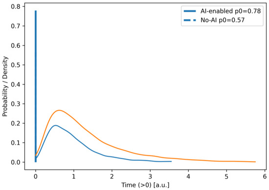
Figure 17.
Review–rework time (loop 97). Mixed distribution with a point mass at zero and a conditional density for positive durations. Vertical spikes at t = 0 show the probability of zero rework time: AI-enabled p0 = 0.78, No-AI p0 = 0.57. Continuous curves show the conditional density f(t∣T > 0). Blue – AI-enabled, orange — No-AI. AI reduces both the frequency (higher p0) and the spread of positive rework times (lower mass in the right tail).
The graph shows a two-component model of post-review revision time. The first component is the point probability of no revisions. For the AI scenario, = 0.78; for the non-AI scenario, p0 = 0.56. There is an increase of +22 percentage points. The second component is the conditional density . In the AI scenario, the peak is closer to zero, and the “tail” is shorter, meaning that if revisions are needed, they last less and are more stable. This is consistent with the decrease in the number of iterations, 9 ↔ 7, and explains the left shift in the total iteration duration (see Figure 4, Figure 5 and Figure 6).
Figure 18 shows the probabilistic dependence of the integration retest time. This figure illustrates the point mass and the conditional density (loop 1110).
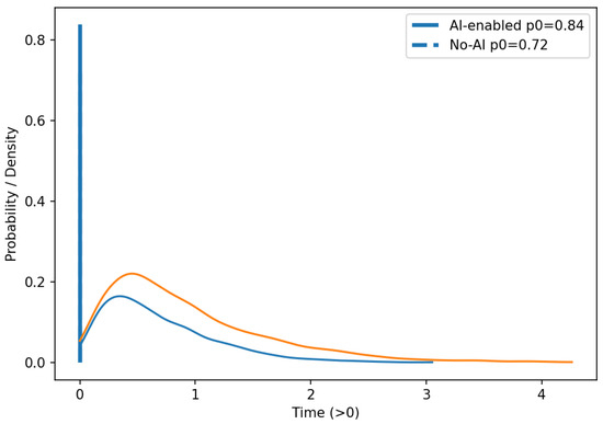
Figure 18.
Two-component distribution of retest time (loop 1110): the vertical sticks at show the point mass (AI-enabled p0 = 0.84; No-AI p0 = 0.72). The blue curve is the conditional density for the AI-enabled scenario; the orange curve is the conditional density for the No-AI scenario. AI increases the zero-mass and shifts the conditional density left, indicating fewer and shorter retests.
The graphs form a vision of the results of the formalization of the two-component model of the rerun time after the integration deployment. In the scenario with the use of AI, the probability that a retest is not needed at all is significantly higher. It is p0 = 0.84 versus p0 = 0.72 in the opposite scenario. We can observe an increase of +12 bp. If a retest occurs (T > 0), its conditional distribution for the scenario with the use of AI is shifted to the left and has a shorter “tail”; that is, the rerun lasts less and is more stable.
Interpretively this, is consistent with the action of AI-enhanced checks at node 8. Some of the problems are cut off to the integration environment, and those that remain require less time to fix. As a result, the effective contribution of the stage to the iteration duration is reduced, which is compactly described by
where in the AI configuration, both factors are smaller [33,34]. The result correlates with the distribution of the number of retests and contributes to the thinner right “tail” of the global duration (see Figure 6 and Figure 7).
Figure 19 shows the curves of the probability dependence of the time of finalization at the reception (arc 12 → 4).
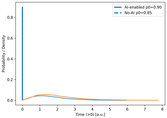
Figure 19.
Two-component distribution of acceptance-rework time (arc 124). Vertical sticks at show (AI-enabled p0 = 0.90; No-AI p0 = 0.85). Blue = AI-enabled conditional density ; orange = No-AI conditional density.
At the final gateway, most increments pass without returning; in the AI scenario configuration, this proportion is higher, p0 = 0.90, compared to the non-AI scenario, p0 = 0.85. If a return occurs (T > 0), the conditional distribution for the AI scenario is shifted to the left and has a shorter “tail”, i.e., corrections last less and are more stable. Visually, the density peak for this scenario is located closer to 1–1.5 CU, while for the non-AI scenario, it is located more to the right, with a more noticeable tail extension to 6–7 CU. The combination of a larger P(T = 0) and a smaller typical duration for T > 0 means a smaller average contribution of the acceptance stage to the total iteration time and further explains the higher probability of meeting deadlines in the AI scenario (see Figure 8).
Results reported above are consistent under our robustness protocol (±10% perturbations; Gamma↔Weibull swaps; Gaussian-copula ; fuzzy weights ±25%), suggesting qualitative stability of deadline reliability and loop attributions.
3.3. Sensitivity and Robustness Analysis
We assess the stability of conclusions under parameter, distributional, dependency, and fuzzy-weight variations (protocol in Section 2.4). Across all tests, the ordering of scenarios remains unchanged: the AI-enabled configuration yields lower median/p90/p95, higher for , and a larger mass at zero for loop PMFs. Quantitative gaps vary (as expected) but do not reverse. We summarize outcomes in Table 9 and provide bootstrap 95% uncertainty bands for representative curves.
Table 9.
Robustness checks–design and qualitative outcomes (95% bootstrap; B = 1000).
4. Discussion
The proposed integrated GERT model of hybrid SDLC with support for I-AND synchronizations and explicit AI nodes interprets the development process as a probabilistic network of interconnected decisions and iterations, in which local changes in the quality of requirements or static code analysis results are translated into global release metrics. The analytical reduction in the network to a W-function provides a transparent comparison of scenarios, in particular “with/without AI”, and allows for the quantitative assessment of the “cost” of review loops, integration retesting, and acceptance returns, while the fuzzy parameterization separates epistemic uncertainty from random variability, making management conclusions interpretable in terms of possible intervals and sensitivities.
This study currently relies on training/synthetic scenarios calibrated from telemetry-like statistics; industrial logs cannot be shared (GDPR/NDAs), which limits external validity. The implicit-AND (I-AND) join is treated as a conservative serialized upper bound; exact join semantics are left for future work and may tighten some results. Calibrations assume process stationarity and Gamma arc durations with Jeffreys-smoothed branch probabilities; heavy tails or seasonality could reduce accuracy. The AI-node mapping (logistic + isotonic) may face covariate shift when toolchains or coding standards change, requiring periodic recalibration. Finally, the framework depends on log completeness and schema mapping (). Missing or biased events can propagate into parameter estimates, and Monte–Carlo runs add moderate CPU cost.
4.1. Assumptions and Threats to Validity
The GERT topology is fixed within an iteration; replications are i.i.d. (no cross-iteration learning). Threat: learning curves. Future work: time-varying parameters.
Outgoing choices at a node and arc times are independent. Threat: hidden common causes. Mitigation: Section 3.3 adds positive correlations (); conclusions stayed stable.
and are time-homogeneous within an iteration. Threat: calendar effects. Future work: non-stationary rates.
No explicit queues/capacity; tasks start when enabled. Scope: elastic CI/CD. Threat: contention-heavy settings. Future work: couple with queueing/GSPN.
At node seven, we use a conservative serialized upper-bound (sum vs. max) to retain a single closed-form W-function. Effect: right-shift in location metrics; Section 2.3 states it; Section 3 shows robustness with unchanged scenario ordering.
For readers new to GERT (Generalized Evaluation and Review Technique), a step-by-step worked example and executable pseudocode illustrating the reduction in a minimal subnetwork with a parallel implicit-AND (I-AND) join and a feedback loop are provided in the Supplementary Materials. The example follows the same semantics as Section 2.3 (conservative serialized I-AND geometric loop reduction) and reuses the probability and Gamma-duration notation of Section 2.4 to keep symbols consistent.
Arc times are Gamma; Mitigation: Section 3.3 replaces Gamma with moment-matched Weibull–ordering preserved.
Telemetry-based mapping to and , fuzzy weights vary by ±25% in Section 3.3 with stable outcomes.
Best suited for instrumented Agile/DevOps iterations with moderate parallelism and elastic infrastructure; extensions are needed for strong resource contention, non-stationary calendars, or high cross-stage dependence.
4.2. External Validation and Scenario Diversity
The sensitivity protocol (Section 2.4 and Section 3.3) indicates that our comparative findings are stable under ±10% parameter changes, Gamma Weibull replacements, moderate inter-stage correlations, and fuzzy-weight variations; bootstrap 95% intervals confirm these effects without reversals.
In the design merge, we replace the physically correct synchronization with the last-finishing branch with a serialized upper-bound approximation (sum). This choice preserves a single closed-form W-function for the entire network and avoids optimistic bias in deadline-related metrics, but it overestimates the merge time. Section 2.3 now states this explicitly, and Section 3 provides a robust note showing that the approximation shifts quantiles to the right and yields a mean overestimation proportional to the faster branch. In future work, we plan to do the following:
- −
- Apply moment-matching/phase-type approximations for the max of gamma variates
- −
- Use hybrid analytic–simulation treatment for parallel gates (exact max on the subnetwork, analytic elsewhere)
- −
- Explore fork–join bounds and numerical inversion for targeted nodes
The assumption of partial independence of transitions and stationarity of process parameters simplifies real interdependence between loops and artifacts. In production environments, return probabilities may be correlated due to expert workloads, domain “blind spots,” or seasonality of requirements
The choice of duration distribution families is likely to depend on the subject area. Universal assumptions require regular validation and, if necessary, re-identification.
The quality of fuzzy sets for epistemic parameters is determined by an expert elicitation procedure; in the absence of standardized protocols, systematic biases are possible, both towards excessive optimism and excessive caution.
Model calibration is based on process telemetry (RE metrics, SAST/CI/CD signals), so its accuracy is sensitive to completeness of logging, consistency of team practices, and data quality; frequent recalibration is required in the event of pivots, staff rotations, or tool changes.
The proposed topology focuses on cause-and-effect relationships and does not explicitly model resource scarcity and queue contention. For certain classes of tasks, this may reduce the accuracy of the forecast without additional consideration of resource constraints.
These limitations form natural directions for further research. One promising approach is to relax the stationarity assumption through online parameter updates and Bayesian calibration, which allows for adaptive accounting of changes in practices and team composition [35,36].
An important step is to extend the fuzzy component to type 2 and formalize elicitation protocols, which will reduce the bias of expert assessments and increase reproducibility. Separate development is required for the identification and cutting off of correlated loops through causal analysis and latent modeling, as well as the introduction of multi-criteria utility functions that integrate time, quality, technical debt, and cost of changes.
In summary, the combination of GERT modeling with I-AND synchronizations, explicit AI nodes, and fuzzy parameterization already provides a comprehensive framework for quantitative management of hybrid software development processes, but its reliability and scope will increase as the outlined shortcomings are overcome and methods for adaptive calibration, resource-process hybridization, and large-scale empirical testing are developed.
We acknowledge that our current evaluation uses a single training/synthetic topology calibrated from telemetry-like statistics. This choice was deliberate: (1) privacy and security constraints prevent sharing raw logs with commit messages, author identifiers, and SAST (Static Application Security Testing) findings; disclosing them would risk leaking secrets or vulnerabilities; (2) legal/organizational approvals (non-disclosure agreements and RODO/General Data Protection Regulation (GDPR) reviews) are ongoing with our partners; (3) schema heterogeneity across repositories (different CI/CD (Continuous Integration/Continuous Delivery) pipelines and log formats) requires a reproducible mapping layer to our GERT arcs (Section 2.4) before fair cross-project comparisons are possible.
As a mitigation, our robustness protocol (±10% parameter perturbations; Gamma–Weibull moment-matched swaps; Gaussian-copula correlations ρ = 0.3 within stage groups; fuzzy weights ±25%; 95% bootstrap confidence intervals) indicates that the headline conclusions (deadline reliability trends and loop attributions) remain qualitatively stable under plausible variations. In future work, we will (1) release a curated, anonymized open-source case with a stable event schema and (2) add two additional topologies (nested rework and highly parallel with conservative I-AND), processed by the same calibration pipeline, to broaden external validity.
5. Conclusions
Thus, a stochastic GERT model of incremental software development with explicit consideration of AI inserts has been developed. The network specifies nodes V = {1,…,13}, arcs with transition probabilities and transformations of duration distributions (W-functions), includes I-AND-union of design results at node seven and three return loops: local 9 ↔ 7 (review), integration 11 ↔ 10 (retest/redeploy), and macrocycle 12 → 4 (return from acceptance). An equivalent W-function with loop reduction has been derived for the entire network, and closed-form expressions for key time metrics (probability of iteration completion, mathematical expectation, and time variance) have been obtained.
The scientific novelty of the model lies in considering AI-activity not as a “superstructure”, but as full-fledged GERT nodes, which allows us to causally trace their influence on the intensity of loops and time distributions. In addition, the model parameters (probabilities of transitions and durations) are presented in a fuzzy formulation for epistemic uncertainty with passing fuzzy sets through formulas according to the expansion principle. This allows us to obtain analytical metrics (e.g., quantiles, survival) and operational derivatives (curves of deadline achievement, contribution of stages), which facilitate managerial interpretation.
An empirical verification and quantitative illustration of a fuzzy GERT model of the development process with explicitly built-in AI inserts was conducted. The experiments showed a consistent effect of AI across the entire range of metrics.
Left shift in the PDF/CDF of the total iteration time and reduction in variability and “long tails”; in the corresponding percentiles, this means a significant reduction of p50/p90/p95 for the AI scenario.
Survival curves (on linear and logarithmic scales) capture tail behavior at large t; the AI-enabled scenario shows uniformly lower tails, reducing planning risk.
The deadline achievement curves show a higher P(T ≤ D) for any practical D; for example, for service level 0.9, the required deadline in the AI configuration is significantly shorter.
The derivative ΔCDF(t) localizes the time interval where the gain from AI is maximum (≈10–12 conditional units) and quantitatively shows the increase in the probability of timely completion (of the order of tens of units).
The anatomy of delays by stage shows that the largest contributions to the win are formed by reducing design time (architecture/UX), automated checks, and a sharp reduction in rework during review, integration, and acceptance.
Discrete metrics (PMF) for the number of loops 9 ↔ 7, 11 ↔ 10, 12 → 4 confirm the shift in the mass to zero and the drop in the probability of multiple repetitions; in the zero-inflated analysis of the time of completions, the mass fraction P(T = 0) increases and the conditional distribution for T > 0 shifts to the left.
In conclusion, the experiments empirically confirmed the analytical conclusions of the model. AI-insertions reduce the intensity of feedback loops and shorten the durations at key stages, which translates into higher chances of meeting deadlines and lower risk of extreme delays at the level of the entire cycle. Importantly, the entire analysis is built on the same formalism (equivalent W-functions/derived metrics) and two reproducible scenarios, so the obtained AI benefits have both statistical and causal interpretations.
We will broaden external validity by adding two representative topologies (nested rework and highly parallel with implicit-AND) and an anonymized open-source case calibrated by the same telemetry pipeline. We plan to move beyond the conservative serialized I-AND by incorporating exact join semantics where synchronization timestamps are available and by quantifying the induced gap empirically. The AI node will be extended to capture dynamic decision policies and the causal impact of SAST/CI signals on rework, with continuous recalibration. We also aim to integrate process-mining discovery and conformance checking to automate arc mapping and detect structural drift, and to model cross-team dependencies plus cost/effort outcomes alongside schedule-risk metrics. Subject to legal approvals (RODO/GDPR), we will release additional anonymized telemetry samples and executable scripts to facilitate replication.
Supplementary Materials
Public repository: https://github.com/serhsemenov/artykl (accessed on 28 October 2025). Contents: README.md (reproduction steps), params_Table3a.csv and params_Table3b.csv (scenario parameters with fuzzy bounds), simulate_gert.py (discrete-event simulator), plot_figs.py (plot generation), make_table5.py (summary metrics), telemetry_sample.csv (synthetic/anonymized schema), and pinned environment files (requirements.txt, environment.yml).
Author Contributions
Conceptualization, S.S. and V.M.; methodology, V.T.; software, V.T.; validation, V.M. and V.T.; formal analysis, S.S. and V.T.; investigation, M.M. (Mateusz Muchacki) and G.L.; data curation, M.M. (Mykhailo Mozhaiev) and V.T.; writing—original draft preparation, S.S. and V.T.; writing—review and editing, S.S. and V.T.; visualization, I.P.; supervision, S.S. and V.T. All authors have read and agreed to the published version of the manuscript.
Funding
This research received no external funding.
Institutional Review Board Statement
Not applicable.
Informed Consent Statement
Not applicable.
Data Availability Statement
The raw data supporting the conclusions of this article will be made available by the authors on request. The study uses training/synthetic scenarios; raw industrial logs are not publicly available due to privacy, security, and legal constraints (RODO/GDPR), but an anonymized open-source case and scenario files will be added to the repository in a subsequent release.
Conflicts of Interest
The authors declare no conflicts of interest.
References
- El Aouni, F.; Moumane, K.; Idri, A.; Najib, M.; Jan, S.U. A systematic literature review on Agile, Cloud, and DevOps integration: Challenges, benefits. Inf. Softw. Technol. 2025, 177, 107569. [Google Scholar] [CrossRef]
- Dong, H.; Dacre, N.; Baxter, D.; Ceylan, S. What is Agile Project Management? Developing a New Definition Following a Systematic Literature Review. Proj. Manag. J. 2024, 55, 668–688. [Google Scholar] [CrossRef]
- Almeida, F.; Bálint, B. Approaches for Hybrid Scaling of Agile in the IT Industry: A Systematic Literature Review and Research Agenda. Information 2024, 15, 592. [Google Scholar] [CrossRef]
- Barros, L.; Tam, C.; Varajão, J. Agile software development projects–Unveiling the human-related critical success factors. Inf. Softw. Technol. 2024, 170, 107432. [Google Scholar] [CrossRef]
- Li, X.-Y.; Liu, Y.; Lin, Y.-H.; Xiao, L.-H.; Zio, E.; Kang, R. A generalized petri net-based modeling framework for service reliability evaluation and management of cloud data centers. Reliab. Eng. Syst. Saf. 2021, 207, 107381. [Google Scholar] [CrossRef]
- Hocaoğlu, M.F. A novel object-oriented Petri net framework with logic programming for discrete and continuous event simulations. Simulation 2025, 101, 951–979. [Google Scholar] [CrossRef]
- Liu, B.; Zhang, H.; Dong, L.; Wang, Z.; Li, S. Metrics for software process simulation modeling. J. Softw. Evol. Process 2024, 36, e2676. [Google Scholar] [CrossRef]
- Guo, C.; Song, Y. A New Stochastic Petri Net Modeling Approach for the Evolution of Online Public Opinion on Emergencies: Based on Four Real-Life Cases. Systems 2024, 12, 333. [Google Scholar] [CrossRef]
- Tao, L.; Su, X.; Javed, S.A. Time-cost trade-off model in GERT-type network with characteristic function for project management. Comput. Ind. Eng. 2022, 169, 108222. [Google Scholar] [CrossRef]
- Zhang, N.; Ou, M.; Liu, B.; Liu, J. A GERT Network Model for input-output optimization of general aviation industry chain based on value flow. Comput. Ind. Eng. 2023, 176, 108945. [Google Scholar] [CrossRef]
- Pregina, K.; Vasugi, K.; Kannan, M.R. Neutrosophic fuzzy-based graphical evaluation and review technique for construction scheduling for residential buildings. Intell. Decis. Technol. 2025, 19, 2267–2294. [Google Scholar] [CrossRef]
- Ahmad, K.; Abdelrazek, M.; Arora, C.; Bano, M.; Grundy, J. Requirements engineering for artificial intelligence systems: A systematic mapping study. Inf. Softw. Technol. 2023, 158, 107176. [Google Scholar] [CrossRef]
- Ferrari, A.; Spoletini, P. Formal requirements engineering and large language models: A two-way roadmap. Inf. Softw. Technol. 2025, 181, 107697. [Google Scholar] [CrossRef]
- Semenov, S.; Kolomiitsev, O.; Hulevych, M.; Mazurek, P.; Chernyk, O. An Intelligent Method for C++ Test Case Synthesis Based on a Q-Learning Agent. Appl. Sci. 2025, 15, 8596. [Google Scholar] [CrossRef]
- Moskalenko, V.; Kharchenko, V.; Semenov, S. Model and Method for Providing Resilience to Resource-Constrained AI-System. Sensors 2024, 24, 5951. [Google Scholar] [CrossRef] [PubMed]
- Figueroa–García, J.C.; Hernández–Pérez, G.; Ramos–Cuesta, J.S. Uncertain project network analysis with fuzzy–PERT and Interval Type–2 fuzzy activity durations. Heliyon 2023, 9, e14833. [Google Scholar] [CrossRef]
- Maravas, A.; Pantouvakis, J.-P. Fuzzy Repetitive Scheduling Method for Projects with Repeating Activities. J. Constr. Eng. Manag. 2011, 137, 561–564. [Google Scholar] [CrossRef]
- Aghileh, M.; Tereso, A.; Alvelos, F.; Lopes, M.O.M. Multi-project scheduling under uncertainty and resource flexibility: A systematic literature review. Prod. Manuf. Res. 2024, 12, 2319574. [Google Scholar] [CrossRef]
- Dotsenko, N.; Chumachenko, I.; Kraivskyi, B.; Railian, M.; Litvinov, A. Methodological support for managing of critical competences in agile transformation projects within a multi-project medical environment. Adv. Inf. Syst. 2024, 8, 26–33. [Google Scholar] [CrossRef]
- Azad, N.; Hyrynsalmi, S. DevOps critical success factors—A systematic literature review. Inf. Softw. Technol. 2023, 157, 107150. [Google Scholar] [CrossRef]
- Kim, G.; Humble, J.; Debois, P.; Willis, J.; Forsgren, N. The DevOps Handbook, 2nd ed.; IT Revolution Press: Portland, OR, USA, 2021. [Google Scholar]
- Saleh, S.M.; Madhavji, N.; Steinbacher, J. A Systematic Literature Review on Continuous Integration and Deployment (CI/CD) for Secure Cloud Computing. In Proceedings of the 20th International Conference on Web Information Systems and Technologies, Porto, Portugal, 17–19 November 2020; pp. 331–341. [Google Scholar]
- Semenov, S.; Liqiang, Z.; Weiling, C. Penetration Testing Process Mathematical Model. In Proceedings of the 2020 IEEE International Conference on Problems of Infocommunications. Science and Technology (PIC S&T), Kharkiv, Ukraine, 6–9 October 2024; pp. 142–146. [Google Scholar]
- Semenov, S.; Lymarenko, V.; Yenhalychev, S.; Gavrilenko, S. The Data Dissemination Planning Tasks Process Model Into Account the Entities Differentity. In Proceedings of the 2022 12th International Conference on Dependable Systems, Services and Technologies (DESSERT), Athens, Greece, 9–11 December 2022; pp. 1–6. [Google Scholar]
- Dong, P.; Chen, W.; Wang, K.; Gong, E. Joint Optimization of Delivery Time, Quality, and Cost for Complex Product Supply Chain Networks Based on Symmetry Analysis. Symmetry 2025, 17, 1354. [Google Scholar] [CrossRef]
- Zhang, N.; Yan, S.; Fang, Z.; Yang, B. Fuzzy GERT model based on z-tag and its application in weapon equipment management. J. Intell. Fuzzy Syst. 2021, 40, 12503–12519. [Google Scholar] [CrossRef]
- Zadeh, L.A. The concept of a linguistic variable and its application to approximate reasoning—I. Inf. Sci. 1975, 8, 199–249. [Google Scholar] [CrossRef]
- Zadeh, L.A. The concept of a linguistic variable and its application to approximate reasoning—II. Inf. Sci. 1975, 8, 301–357. [Google Scholar] [CrossRef]
- Zadeh, L.A. The concept of a linguistic variable and its application to approximate reasoning—III. Inf. Sci. 1975, 9, 43–80. [Google Scholar] [CrossRef]
- Semyonov, S.G.; Gavrilenko, S.Y.; Chelak, V.V. Information processing on the computer system state using probabilistic automata. In Proceedings of the 2017 2nd International Ural Conference on Measurements (UralCon), Chelyabinsk, Russia, 16–19 October 2017; pp. 11–14. [Google Scholar]
- Silverman, B.W. Density Estimation for Statistics and Data Analysis, 1st ed.; CRC Press: Boca Raton, FL, USA, 1986; Volume 26. [Google Scholar]
- Feng, C.X. A comparison of zero-inflated and hurdle models for modeling zero-inflated count data. J. Stat. Distrib. Appl. 2021, 8, 8. [Google Scholar] [CrossRef] [PubMed]
- Almeida, Y.; Albuquerque, D.; Filho, E.D.; Muniz, F.; Santos, K.d.F.; Perkusich, M.; Almeida, H.; Perkusich, A. AICodeReview: Advancing code quality with AI-enhanced reviews. SoftwareX 2024, 26, 101677. [Google Scholar] [CrossRef]
- Charoenwet, W.; Thongtanunam, P.; Pham, V.-T.; Treude, C. Toward effective secure code reviews: An empirical study of security-related coding weaknesses. Empir. Softw. Eng. 2024, 29, 88. [Google Scholar] [CrossRef]
- Li, J.; Deng, Z.; Tang, Y.; Wang, S.; Yang, Z.; Luo, H.; Feng, W.; Zhang, B. Improved Bayesian Model Updating Method for Frequency Response Function with Metrics Utilizing NHBFT-PCA. Mathematics 2024, 12, 2076. [Google Scholar] [CrossRef]
- Meleshko, Y.; Raskin, L.; Semenov, S.; Sira, O. Methodology of probabilistic analysis of state dynamics of multidimensional semiMarkov dynamic systems. East. Eur. J. Enterp. Technol. 2019, 6, 6–13. [Google Scholar] [CrossRef]


Disclaimer/Publisher’s Note: The statements, opinions and data contained in all publications are solely those of the individual author(s) and contributor(s) and not of MDPI and/or the editor(s). MDPI and/or the editor(s) disclaim responsibility for any injury to people or property resulting from any ideas, methods, instructions or products referred to in the content. |
© 2025 by the authors. Licensee MDPI, Basel, Switzerland. This article is an open access article distributed under the terms and conditions of the Creative Commons Attribution (CC BY) license (https://creativecommons.org/licenses/by/4.0/).