Abstract
Avalanche susceptibility mapping is vital for disaster prevention and infrastructure safety in cold mountain regions under climate change. Traditional machine learning (ML) approaches have demonstrated strong predictive capacity, yet their limited interpretability and difficulty in identifying threshold effects hinder their broader application in geohazard risk management. To overcome these limitations, this study develops an explainable ML framework that integrates remote sensing data, topographic and climatic variables, and SHapley Additive exPlanations for the Kanas Scenic Area transportation corridor in the Chinese Altay Mountains. The framework evaluates five classifiers: Random Forest, XGBoost, LightGBM, Soft Voting, and Stacking, and using sixteen conditioning factors that capture topography, climate, vegetation, and anthropogenic influences. Results show that LightGBM achieved the best performance, with an AUC of 0.9428, accuracy of 0.8681, F1-score of 0.8750, and Cohen’s kappa of 0.7366. To ensure transparency for risk decisions, SHAP analyses identify Terrain Ruggedness Index, wind speed, slope, aspect and NDVI as dominant drivers. The dependence plots reveal actionable thresholds and interactions, including a TRI plateau near 5–7, a slope peak between 30° and 40°, a wind effect that saturates above about 2.5 m s−1, and a near-river high-risk belt within 0–2 km. The five-class map aligns with independent field observations, with more than three quarters of events falling in moderate to very high zones. By integrating explainable ML with remote sensing, this study advances avalanche risk assessment in cold region transportation corridors and strengthens the robustness of regional susceptibility mapping.
1. Introduction
Avalanches, as a distinctive type of geohazard in cold mountainous regions, are rapid downslope movements of snow masses triggered by the sudden collapse of unstable snowpacks. They pose severe threats to human life, transportation corridors, and alpine infrastructure [1,2,3]. Their occurrence typically results from the combined influence of steep terrain, wind-driven snow deposition, heavy snowfall, sharp temperature fluctuations, and insufficient vegetation anchoring [4,5]. In mountainous regions—especially along remote transportation corridors—sudden avalanches can sever vital routes and isolate communities [6,7]. Ongoing climate warming and more frequent extremes further elevate avalanche risk on mountain roads, as rising temperatures, snowpack instability, and altered precipitation regimes increase both the frequency and unpredictability of events [8,9]. Avalanches typically arise in cold mountainous environments where sustained snow accumulation, low temperatures, and strong winds interact to form unstable snow layers. Prolonged subfreezing conditions promote weak layers through faceting and depth-hoar growth, while intermittent thaw–freeze cycles and wind deposition enhance snowpack stratification. Subsequent loading or temperature variations can then cause shear stress to exceed snow cohesion, triggering avalanches. Northern Xinjiang’s Altay Mountains exemplify such an avalanche-prone setting: lasting snow cover, high winds, and large diurnal temperature ranges accelerate snow metamorphism and instability. In mid–high latitudes such as China’s Altai Mountains, frequent avalanches have been documented along roads in the Kanas Scenic Area; for example, multiple avalanches on 8 January 2024 caused road closures and stranded thousands of visitors. Avalanche susceptibility mapping—which delineates areas prone to future avalanches from environmental and climatic indicators—is a powerful tool for infrastructure planning, early warning, and disaster mitigation in vulnerable mountain corridors [10]. Because susceptibility is strongly conditioned by local terrain, climate, and surface characteristics, region-specific modeling is essential. A deeper understanding of the physical mechanisms and spatiotemporal patterns of avalanche occurrence not only improves prediction accuracy but also supports targeted mitigation strategies and reliable risk zoning for fragile mountain corridors [11].
The growing availability of high-resolution topographic data, meteorological reanalysis products, and advanced data processing has made Geographic Information Systems (GIS) and Remote Sensing (RS) indispensable for detailed spatiotemporal analyses of avalanche susceptibility [12]. GIS and RS enable the extraction of high-quality topographic, surface, and climatic variables at fine spatial resolutions, providing critical inputs for susceptibility modeling and risk mapping [13]. To address the complexity of mountain environments, a broad spectrum of modeling approaches has been developed, typically grouped into physical, statistical, and ML methods. Physical models such as RAMMS and SNOWPACK simulate avalanche release and runout using snow mechanics, mass-movement theory, and dynamic flow equations [14,15]. Statistical approaches including Frequency Ratio (FR), Information Value (IV), and Certainty Factor (CF) quantify empirical relationships between historical avalanches and conditioning factors within multi-criteria frameworks [16]. In addition to conventional statistical approaches, multi-criteria decision analysis (MCDA) frameworks have also been applied for avalanche susceptibility mapping, where factor weights are determined through expert judgment or analytical hierarchy processes [17]. While statistically based models are relatively simple and interpretable, they often struggle to capture the inherently nonlinear interactions that govern avalanche processes [18].
In recent years, ML has emerged as a powerful alternative due to its capability to handle high-dimensional, multi-source, and strongly interacting datasets [19]. Unlike rule-based or traditional statistical methods, data-driven ML models can effectively learn nonlinear relationships between avalanche occurrence and conditioning factors such as terrain characteristics, snow accumulation patterns, and meteorological influences. A range of classifiers—e.g., Logistic Regression (LR) [20], Support Vector Machine (SVM) [21], Multiple Discriminant Analysis (MDA) [22], and Generalized Additive Model (GAM) [23]—have been used individually to produce susceptibility maps with promising skill. Recent studies highlight that ensemble learning further improves accuracy by aggregating the strengths of multiple classifiers [24,25]. For instance, Akay demonstrated the effectiveness of tree-based ensemble algorithms in Turkey’s alpine regions [26], while Iban and Bilgilioglu employed XGBoost and SHAP to interpret avalanche susceptibility across spatial scales [27]. Similarly, Liu et al. and Fang et al. integrated ensemble learning with factor analysis to improve prediction reliability in mountainous environments [28,29]. These works collectively represent the state of the art in data-driven avalanche modeling, yet they remain primarily focused on predictive performance rather than interpretability. Consequently, the lack of a unified explainable framework limits the operational use of ML models in practical risk assessment. Among these, tree-based methods such as Random Forest (RF), eXtreme Gradient Boosting (XGBoost), and Light Gradient Boosting Machine (LightGBM) achieve notable gains in accuracy and stability [27,30]. Additional ensemble strategies, such as Soft Voting and Stacking, have also been explored to further optimize predictive performance [31]. Despite their strong predictive skills, conventional ML models often struggle to explain complex variable interactions and spatial heterogeneity of triggers in mountains. Limited transparency and physical interpretability can reduce credibility and usability in operational risk management, particularly in highly heterogeneous cold regions. Addressing this interpretability gap is therefore critical to bridge the divide between data-driven predictions and physically meaningful avalanche processes.
To improve model transparency and trustworthiness, explainable artificial intelligence (XAI) has attracted increasing attention [32]. Among XAI techniques, SHapley Additive exPlanations (SHAP) is particularly effective, as it quantifies the marginal contribution of each conditioning factor to model predictions based on cooperative game theory and provides both global and local explanations through summary and dependence plots [33]. Compared with conventional feature importance measures, SHAP enhances interpretability by not only ranking variables but also revealing nonlinear responses and interactive effects, thereby aligning model outputs with physical processes relevant to avalanche initiation and runout [34]. Previous research has made significant progress in applying ML to avalanche susceptibility modeling, achieving higher predictive accuracy through ensemble methods and multi-source data integration. However, most studies have primarily focused on improving model performance rather than interpretability. Even when explainable methods such as SHAP have been adopted, their application has largely been limited to displaying global feature importance, without further exploring localized threshold effects, nonlinear responses, or cross-factor interactions that govern avalanche formation [35]. This gap prevents current models from providing physically meaningful insights or supporting real-world monitoring and early warning. Addressing this interpretability challenge represents a critical step toward bridging data-driven prediction with process understanding.
Building on these developments, this study proposes an integrated and interpretable avalanche susceptibility modeling framework that combines multiple ensemble ML classifiers with a SHAP-based explanatory approach. The framework is applied to the Kanas Scenic Area transportation corridor in the Altay Mountains, northwestern China, aiming to (1) evaluate and compare the performance of advanced ensemble learning algorithms under complex alpine conditions, (2) enhance model interpretability by quantifying threshold effects and factor interactions using SHAP, and (3) generate a high-resolution susceptibility map aligned with field validation to support disaster prevention and infrastructure planning in cold mountain regions..
2. Study Area
The study area is the Kanas Scenic Area in northern Altay City, Xinjiang, China (Figure 1), located on the southern flank of the Altai Mountains (48°30′20″ N, 87°07′37″ E). The Altai range extends from 85°54′ to 90°58′ E and from 45°37′ to 49°10′ N, spanning nearly 500 km within China. Relief exhibits a pronounced NW–SE gradient, with Youyi Peak reaching 4374 m and valley floors descending to ~1000 m, forming a stepped landscape of glaciated highlands, steep midslopes, and dissected piedmonts. Kanas Scenic Area is characterized by deep-incised gorges, marked elevational contrasts, and clear altitudinal vegetation belts that include glacial and periglacial zones, coniferous forests, alpine meadows, and semi-arid shrublands.
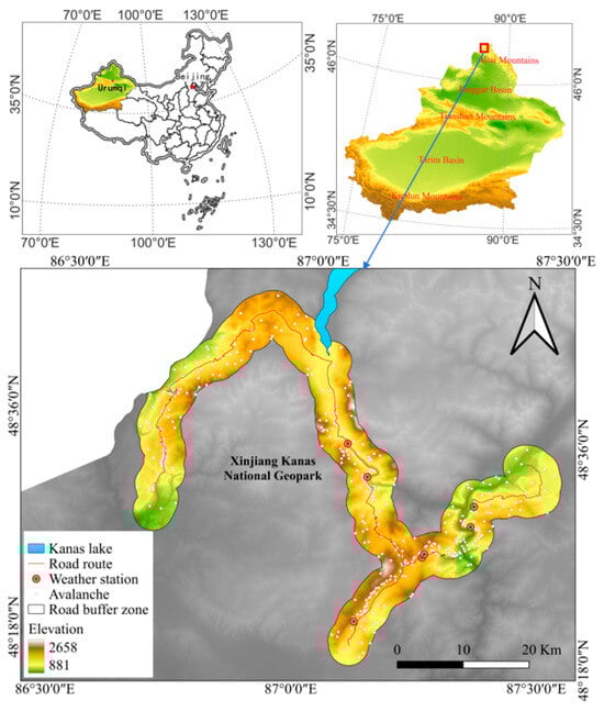
Figure 1.
Location map of the study area. The red rectangle marks the Kanas Scenic Area, and the blue arrow indicates the zoomed-in direction. The lower panel shows the road network, avalanche points, and weather stations within the Xinjiang Kanas National Geopark.
The region experiences a cold-temperate climate characterized by long, severe winters and a short growing season. Situated deep within the Eurasian continent and far from maritime moisture sources, and further influenced by complex topography, it develops distinctive microclimates. The mean annual temperature is −0.2 °C, with winter extremes down to about −40 °C. Mean annual precipitation is ~1000 mm, over 70% of which falls during the warm half of the year. Winters (October–April) are dominated by persistent snow cover, with >70 snowfall days annually and a snow season lasting >200 days. Snowfall typically begins in late August above 1400 m, and seasonal snow depth can reach 1–2 m.
From the perspective of avalanche susceptibility, Kanas Scenic Area presents a highly vulnerable snow-hazard environment. Steep terrain, heterogeneous forest cover, intense convective snowfall, and strong wind redistribution during the snow season jointly create conditions conducive to avalanche occurrence. Major transportation corridors and associated tourist infrastructure traverse known avalanche-prone zones and face direct impact risk. Recent events have not only interrupted traffic but also underscored the urgent need for predictive avalanche mapping. The region’s climatic and geomorphic setting makes it a natural testbed for applying remote sensing and explainable machine learning to avalanche susceptibility analysis.
3. Materials and Methods
3.1. Avalanche Inventory
An avalanche inventory is a prerequisite for susceptibility modeling: it provides georeferenced records of past events and serves as the dependent variable for model training and validation. All avalanche samples were randomly partitioned using an 80/20 split, with 80% allocated to the training set for model fitting and 20% reserved for the test set for independent performance evaluation. During the 2023–2024 snow season, 226 avalanche events were documented within the Kanas Scenic Area. The inventory was compiled primarily from field surveys and on-site unmanned aerial vehicle (UAV) campaigns (Figure 2).
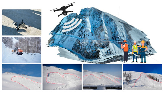
Figure 2.
UAV imagery illustrating site conditions and observed avalanche morphological features.
Field observations were conducted following major snowfall events, focusing on road corridors along the S232, X852, and G219 highways where avalanche activity is common. Ground records included geotagged photographs, GPS-delineated outlines of avalanche debris, and visual confirmation of crown fracture lines and runout paths. In selected high-hazard areas, UAV-based photogrammetry was employed to validate satellite-derived detections and to refine debris boundaries in steep and forested terrain [36]. High-resolution terrain data were acquired using a DJI Matrice 300 RTK UAV equipped with a Zenmuse H20 camera (DJI, Shenzhen, China). The flight altitude was 500 m, with 80% longitudinal and 70% lateral overlap. The resulting 0.2 m DEM and DOM.
The final avalanche dataset was converted to point-format centroid coordinates representing initiation or release areas. Each point was assigned a binary label, and an equal number of non-avalanche points was randomly sampled from slopes with no observed activity to ensure class balance. All points were then linked to topographic, vegetation, and meteorological predictors extracted from the geospatial database for avalanche susceptibility modeling. The performance of all models was evaluated using the 20% test subset of the avalanche inventory, which included 45 independent avalanche events randomly selected from the 2023–2024 snow season. These unseen samples were used exclusively for quantitative performance assessment (AUC, F1, κ, and accuracy), ensuring unbiased validation of the predictive models.
3.2. Avalanche Conditioning Factors
Selecting factors for avalanche susceptibility modeling requires careful consideration of local environmental complexity, dominant triggering mechanisms, data availability, and the need for model interpretability [23]. In the Kanas Scenic Area, avalanche occurrence is primarily influenced by the combined effects of slope steepness, snow accumulation and wind-driven redistribution, vegetation cover, and meteorological extremes. Guided by expert knowledge from regional avalanche monitoring and control, evidence from prior studies, and data accessibility, we selected 16 conditioning factors that are mechanistically linked to local avalanche processes. These variables capture potential instability mechanisms across topographic setting, snow distribution, climatic forcing, and vegetation conditions, and align with dominant triggers such as slope breaks, wind transport, and intense snowfall.
The selected factors include: topographic metrics—elevation, slope, aspect, curvature, plan curvature (PlanCurv), profile curvature (ProfCurv), local terrain relief (Relief), Topographic Wetness Index (TWI), Topographic Position Index (TPI), and Terrain Ruggedness Index (TRI); surface and vegetation indicators—distance to rivers (DistRiver), land use (LU), and Normalized Difference Vegetation Index (NDVI); and snow-season meteorological variables—daily maximum air temperature (Tmax), precipitation (Precip), and maximum wind speed (MaxWind).
3.2.1. Data Sources
Table 1 summarizes the datasets used to derive the 16 conditioning factors. Ten terrain variables—elevation, slope, aspect, curvature, ProfCurv, PlanCurv, Relief, TWI, TPI, and TRI—were extracted from the 12.5 m ALOS PALSAR digital elevation model (DEM) using the Spatial Analyst tools in ArcGIS 10.8. The NDVI layer was obtained from NASA’s MOD13A3 monthly NDVI composite. Land use information was taken from the China Land Cover Dataset (CLCD) at 30 m resolution, developed by Wuhan University from annual Landsat observations [37].

Table 1.
Data and data sources.
Snow-season meteorological variables included Tmax, Precip, and MaxWind, retrieved from the ERA5-Land reanalysis provided via the Copernicus Climate Data Store. River polylines were sourced from the National Earth System Science Data Center and used to compute a Euclidean DistRiver. Because the native spatial resolutions differ markedly across sources, all raster datasets were harmonized to 12.5 m to avoid scale mismatch and interpolation artifacts. Continuous variables were resampled using bilinear interpolation, whereas categorical layers were resampled using nearest-neighbor to preserve class integrity. The resampled products underwent visual cross-checks and consistency assessments to ensure conformity with the original spatial patterns, thereby improving factor-layer coherence and the reliability of inputs for susceptibility modeling.
All spatial layers were projected to the WGS 1984 UTM Zone 45N coordinate system to ensure spatial consistency. Raster layers were resampled to a uniform resolution of 12.5 m using bilinear interpolation and overlaid using the spatial analyst tools in ArcGIS 10.8. Factor extraction for each avalanche and non-avalanche point was conducted through the “Extract Multi Values to Points” tool, ensuring a one-to-one correspondence between sample points and conditioning variables. The Kanas Scenic Transportation Corridor, covering highways S232, X852, and G219, was delineated using road vector data with a 3 km buffer zone to define the analysis area. Avalanche and non-avalanche samples were extracted within the buffered corridor through overlay analysis for model training. Topographic predictors for susceptibility mapping were derived from the 12.5 m ALOS PALSAR DEM, whereas UAV-derived DOM/ ≈ 0.2 m DEM were used only for site-specific mapping and validation of avalanche outlines and were not included as model predictors. Statistical modeling was implemented in Python 3.10(scikit-learn/XGBoost, fixed random seed) using a 1:1 presence–background sample and an 80/20 train–test split.
3.2.2. Topographic and Vegetation Factors
Topographic characteristics strongly influence snow deposition, wind-driven redistribution, and the physical conditions that lead to avalanche release. The factors considered here include elevation, slope, aspect, curvature, ProfCurv, PlanCurv, local relief (Relief), TWI, TPI, and TRI (Figure 3). Figure 3a depicts the elevation distribution across the study area; elevation modulates snow depth, temperature variability, and the duration of seasonal snow cover, particularly in high basins with limited insolation [38]. Slope is a primary determinant of gravitational instability [39]; avalanche-prone slopes typically fall within 25–45°, where shear stress exceeds the shear strength of the snowpack [40]. Aspect influences formation processes by regulating melt rates and exposure to storms; leeward slopes commonly receive wind-deposited snow, whereas sun-exposed slopes may wet earlier—both pathways can promote instability [41].
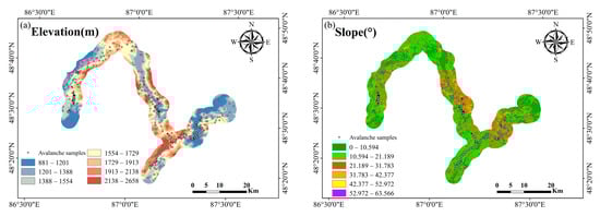
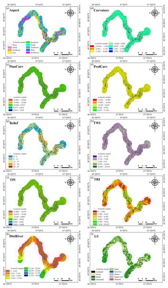
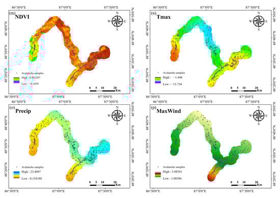
Figure 3.
Thematic map of avalanche conditioning factors (a) Elevation; (b) Slope; (c) Aspect; (d) Curvature; (e) PlanCurv; (f) ProfCurv; (g) Relief; (h) TWI; (i) TPI; (j) TRI; (k) DistRiver; (l) LU; (m) NDVI; (n) Tmax; (o) Precip; (p) MaxWind.
Curvature metrics (Curvature, ProfCurv, PlanCurv) capture surface geometry and shape spatial patterns of snow accumulation and drainage. Concave slopes tend to accumulate snow, while convex breaks often serve as release zones [42]. Relief, TPI, and TRI characterize local variability and prominence, which are closely linked to potential release areas and terrain traps. Finally, NDVI indicates vegetation density: low NDVI typically reflects sparse cover or bare ground that provides limited mechanical anchoring and is more susceptible to overloading, whereas higher NDVI on forested slopes can enhance stability by intercepting snowfall and reducing wind exposure.
3.2.3. Meteorological Factors
Meteorological forcing is a primary trigger of avalanche events and largely governs the timing and magnitude of releases. Three variables were considered: snow-season daily maximum air temperature, seasonal cumulative precipitation, and maximum wind speed. These fields were obtained from ERA5-Land and downscaled to 12.5 m using inverse distance weighting to produce the grids shown in Figure 3. Tmax regulates the thermal state of the snowpack; sustained temperatures above 0 °C promote meltwater percolation, loss of cohesion, and wet-snow avalanches [43]. Precip represents moisture input and loading; intense or persistent precipitation increases overburden and may initiate failure, while rain-on-snow under near-freezing conditions can accelerate weakening. MaxWind is particularly important in mountains, where strong winds transport snow from windward to leeward slopes, forming dense, cohesive slabs and cornices that are often unstable and prone to collapse [44]. Together, these meteorological variables capture dynamic atmospheric conditions that interact with static topography to control avalanche occurrence, and their inclusion improves representation of both background and triggering conditions in susceptibility modeling.
All topographic and vegetation variables represent static conditions, while meteorological factors were composited from two consecutive snow seasons (November–April 2022/2023 and 2023/2024) to ensure temporal consistency with the recorded avalanche events. This temporal alignment ensures that the remote-sensing–derived predictors correspond directly to the period of avalanche occurrence. Meteorological factors were derived from ERA5-Land for two recent snow seasons (November–April 2022/23 and 2023/24) and composited to match the 2023/24 avalanche inventory period.
3.3. Methodology
This study followed five main steps. First, avalanche and non-avalanche samples were prepared from field surveys and UAV data, and 16 conditioning factors were extracted using GIS. Second, multicollinearity among factors was assessed with Pearson’s correlation and the variance inflation factor (VIF) to ensure model robustness. Third, five classifiers—RF, XGBoost, LightGBM, Soft Voting ensemble, and Stacking ensemble—were trained and evaluated using stratified sampling and multiple performance metrics. Fourth, the SHAP framework was applied to interpret feature contributions at global and local scales. Finally, the best-performing model was used to produce the avalanche susceptibility map, and the predicted probabilities were partitioned into five susceptibility classes for spatial visualization. Figure 4 summarizes the workflow.
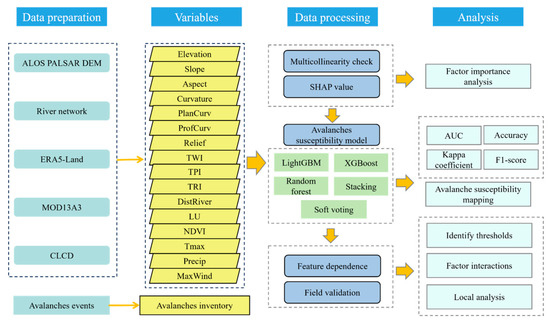
Figure 4.
Schematic diagram of the workflow of this study.
3.3.1. LightGBM
LightGBM is an efficient tree-based ensemble learning algorithm developed to improve the training speed, scalability, and accuracy of gradient boosting frameworks [45]. It builds decision trees in a leaf-wise manner rather than level-wise, prioritizing the leaf with the highest loss reduction, which enhances convergence and allows the model to capture complex feature interactions more effectively.
The model iteratively fits a series of regression trees to the residuals of previous predictions by minimizing a regularized objective function. The general formulation of the additive model is expressed as:
where denotes the regression tree added at the -th iteration and is the corresponding learning rate. Each tree is constructed to optimize a second-order Taylor approximation of the loss function, which incorporates both gradient and Hessian information. Regularization terms are included to control model complexity and mitigate overfitting.
LightGBM introduces two novel techniques—gradient-based one-side sampling (GOSS) and exclusive feature bundling (EFB)—to reduce computational cost without compromising model accuracy. GOSS retains instances with large gradients while randomly sampling from those with small gradients, accelerating convergence. EFB bundles mutually exclusive features to reduce dimensionality, particularly beneficial in high-dimensional sparse datasets.
In this study, LightGBM was employed to construct the avalanche susceptibility model using a set of 16 environmental predictors, including topographic, meteorological, and vegetation-related factors. The model was trained using stratified sampling to address class imbalance, and missing values were handled through median imputation. Hyperparameters were optimized via manual tuning and cross-validation, with the number of trees set to 300, the learning rate to 0.05, and the maximum tree depth to 5.
3.3.2. Random Forest
Random Forest is a bagging-based ensemble method that constructs multiple decision trees using bootstrapped samples of the training data [46]. Each tree is built independently, and predictions are aggregated through majority voting to reduce variance and improve generalization. The final output is given by:
where denotes the prediction of the -th tree and is the total number of trees. In this study, the RF model consisted of 300 trees with a maximum depth of 15. Balanced class weights were applied to address data imbalance, and missing values were handled by median imputation. RF was included as a robust baseline due to its tolerance to multicollinearity and ability to assess variable importance.
3.3.3. XGBoost
XGBoost is a scalable and regularized variant of the traditional gradient boosting algorithm, designed for efficient learning on structured data [47]. Like other boosting methods, XGBoost builds an ensemble of weak learners in a stage-wise manner, where each new tree is trained to minimize the residual error of the ensemble’s current predictions.
XGBoost introduces several improvements, including shrinkage, column subsampling, and explicit regularization terms, which help to control overfitting and enhance model generalization. The regularized objective function is defined as:
Here, is the loss function, penalizes model complexity via the number of leaves and their weights , and , are regularization coefficients.
In this study, the XGBoost model was configured with 150 trees, a learning rate of 0.08, and a maximum depth of 5. Feature preprocessing and sampling procedures were aligned with those used in the RF and LightGBM models. The inclusion of XGBoost enables comparison with other boosting and bagging algorithms under a consistent framework.
3.3.4. Stacking Ensemble
Stacking is a meta-learning strategy that integrates the predictions of multiple base classifiers by training a higher-level learner to combine them. In this study, logistic regression was used as the meta-learner, while LightGBM, XGBoost, and RF served as base learners. During training, out-of-fold predictions from the base learners were used as input features to the meta-learner, which helps reduce overfitting and improve generalization. The stacking ensemble enables the complementary strengths of different algorithms to be leveraged within a unified framework.
3.3.5. Soft Voting Ensemble
The soft voting ensemble aggregates the probabilistic outputs of multiple classifiers by computing the weighted average of predicted class probabilities. In this study, equal weights were assigned to LightGBM, XGBoost, and RF. The final class label was determined by selecting the class with the highest average probability. Soft voting is particularly effective when individual models exhibit diverse yet complementary decision boundaries, and it enables performance gains with minimal additional complexity.
3.3.6. Shapley Additive Explanation
To enhance the interpretability of avalanche susceptibility models, this study employed SHAP, a unified framework based on cooperative game theory. SHAP quantifies the marginal contribution of each predictor to individual predictions by computing Shapley values, which represent the average marginal contribution of a feature across all possible coalitions [48].
Given a trained model , the SHAP value for feature is calculated as:
where is the set of all input features, and is a subset of features not containing . This formulation ensures local accuracy, consistency, and missingness.
We used the TreeSHAP algorithm to compute SHAP values for each test sample, attributing model outputs to individual features. TreeSHAP provides computational efficiency and exact attribution for tree ensembles, making it suitable for high-dimensional inputs. We then generated global and local SHAP plots based on all 226 avalanche instances, visualizing the average influence of each input and the marginal interaction patterns, and thereby identifying the key determinants of avalanche susceptibility. Feature importance was ranked by the mean absolute SHAP values, and no fixed threshold was imposed.
3.4. Performance Assessment
The performance of avalanche susceptibility classifiers was assessed using four widely adopted evaluation metrics: overall accuracy (Acc), F1-score, Cohen’s kappa coefficient (κ), and the area under the receiver operating characteristic curve (AUC). These indicators provide complementary perspectives on model reliability and are particularly suited for imbalanced datasets common in avalanche occurrence. The formulas are defined as follows:
In these equations, TP (true positives) and TN (true negatives) denote avalanche and non-avalanche instances correctly classified, respectively, while FP (false positives) and FN (false negatives) represent misclassifications.
Accuracy reflects overall classification correctness. The F1-score provides a balanced measure of precision and recall, making it robust for uneven avalanche-to-non-avalanche ratios. Cohen’s kappa quantifies the level of agreement between predictions and observations beyond chance expectation. AUC is derived from the receiver operating characteristic (ROC) curve and measures the threshold-independent discriminative capacity of a model; values close to 1 indicate excellent separability, whereas values near 0.5 imply random performance.
4. Results
4.1. Multicollinearity Results
To evaluate potential multicollinearity among the 16 conditioning factors, we computed the Pearson correlation matrix and VIFs. As shown in Figure 5, the meteorological variables—Precip, Tmax, and MaxWind—exhibit relatively high VIFs, approaching or slightly exceeding the commonly used threshold of 10, indicating moderate to high multicollinearity. By contrast, most terrain and land-cover variables, such as NDVI, LU, and curvature, have low VIFs (<4), suggesting minimal redundancy. Despite the elevated VIFs for the meteorological set, these variables were retained due to their theoretical relevance to avalanche formation in cold regions and their expected contribution to model skill. Moreover, the mean VIF across all factors remains within acceptable bounds, and no variable showed excessive inflation warranting exclusion.
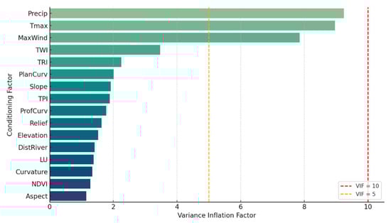
Figure 5.
VIF values of the 16 avalanche conditioning factors.
The Pearson correlation matrix (Figure 6) corroborates these findings. While most factor pairs show weak-to-moderate associations (|r| < 0.7), several expected geometric linkages are evident. For example, slope correlates strongly with Relief (r = 0.97) and TRI (r = 0.99), and TPI correlates with PlanCurv (r = 0.83) and overall curvature (r = 0.96). Linear relationships between meteorological and topographic variables are limited, implying complementary roles in the model. Although some multicollinearity is present, no variables were removed. This decision reflects the use of tree-based ensemble classifiers, which are nonparametric and split-based and are inherently robust to multicollinearity. Retaining all 16 factors also enables a more comprehensive assessment of feature contributions in the subsequent SHAP interpretability analysis.
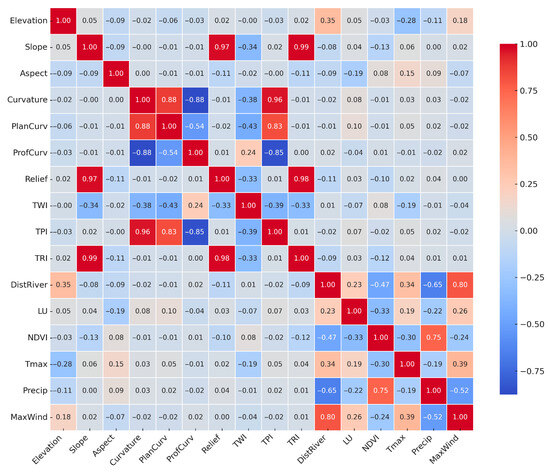
Figure 6.
Pearson’s correlation coefficient matrix.
4.2. Classifier Performance
To assess the predictive capabilities of different models in avalanche susceptibility mapping, five classifiers were evaluated: XGBoost, RF, LightGBM, Soft Voting, and Stacking. Each model was trained and tested using a stratified split (80% training, 20% testing), and performance was evaluated based on AUC, Acc, F1-score, and Kappa coefficient, the specific results are shown in Figure 7.
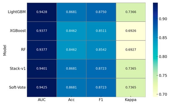
Figure 7.
Classifiers’ performance comparison.
LightGBM outperformed the other classifiers, achieving the highest AUC (0.9428), accuracy (0.8681), F1-score (0.8750) and Kappa coefficient (0.7366), indicating its superior ability to distinguish between avalanche-prone and non-prone areas. XGBoost and RF exhibited comparable performance with AUCs of 0.938, Acc of 0.8462, and slightly lower Kappa values (0.692). The ensemble classifiers, including the Soft Voting and Stacking models, also demonstrated strong performance, with the Stacking model reaching an AUC of 0.943 and balanced scores across all evaluation metrics.
The ROC curves (Figure 8) further illustrate the discriminative power of the models. All classifiers showed good separation capability, with ROC curves closely following the upper-left boundary of the plot, confirming the robustness of tree-based ensemble methods in avalanche susceptibility modeling.
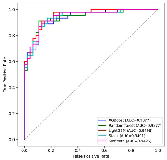
Figure 8.
ROC curves.
4.3. SHAP-Based Feature Importance
The SHAP summary plot and feature importance ranking of the LightGBM model are shown in Figure 9a and Figure 9b, respectively. These results reveal the contribution and direction of each conditioning factor to avalanche susceptibility across the entire study area.
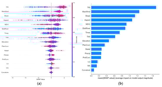
Figure 9.
Schematic diagram of feature ranking (a) Summary plot of SHAP values; (b) Factor importance plot.
Figure 9a illustrates the SHAP summary plot derived from the LightGBM model, highlighting the relative importance and directional influence of the 16 conditioning factors used in avalanche susceptibility modeling. Each dot represents an individual sample, with its horizontal position indicating the corresponding SHAP value and its color denoting the original feature value. Red dots indicate higher feature values, whereas blue dots represent lower values. From top to bottom, the features are ranked according to their mean absolute SHAP values (Figure 9b).
The top five most influential variables are TRI, maximum wind speed, slope, aspect, and NDVI, all of which exert significant impacts on the model output. Among them, TRI was identified as the most influential factor, suggesting that areas with greater terrain variability are more prone to avalanches. Maximum wind speed also plays a critical role, reflecting the importance of wind redistribution in snow loading and slab formation—both of which are central to avalanche triggering mechanisms. Slope ranks third, aligning with established understanding that avalanches are more likely to occur on moderately steep to steep slopes, particularly between 30° and 45°. Aspect and NDVI also exhibit substantial influence. South-facing slopes, which receive greater solar radiation, and areas with sparse vegetation are more susceptible to surface instability due to snowpack weakening or lack of anchorage. In contrast, variables such as curvature, TPI, and land use show narrow SHAP value distributions and lower importance, indicating limited contributions to the model. Interestingly, several factors, including precipitation and elevation, display both positive and negative SHAP effects across their value ranges, reflecting their nonlinear roles and environmental dependence in avalanche initiation.
4.4. SHAP Dependence Plots
To reveal the nonlinear responses and pairwise interactions between conditional factors, the study used TreeSHAP to calculate SHAP values and plot dependency diagrams. Primary variables were selected by global importance and mechanistic relevance. For each primary variable, the secondary variable used for coloring was chosen based on the strongest interaction signal together with physical interpretability; when multiple candidates were comparable, we preferred combinations that produced clearer color gradients and aligned with known avalanche processes. In each plot, the x-axis is the raw value of the primary variable, the y-axis is its SHAP value, and point colors encode the secondary variable, which allows simultaneous inspection of the marginal effect and its modulation.
Figure 10a shows a strong positive relationship between TRI and SHAP values. The contribution increases rapidly and reaches a plateau at approximately 5–7, with limited marginal gains beyond about 7. Steeper slopes amplify the positive effect most clearly when slope is at least 30°, whereas slopes of 15° or less markedly weaken the TRI gain. Figure 10b indicates a generally monotonic increase in SHAP with maximum wind speed and a saturation at higher values. The contribution changes sign near 2.0–2.3 m s−1 and then levels off for values above about 2.5 m s−1. Larger TRI values are associated with stronger positive wind effects; lower TRI weakens them.
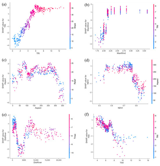
Figure 10.
SHAP dependency plots of different principal factors with their interactors: (a) TRI–Slope, (b) MaxWind–TRI, (c) Aspect–Relief, (d) NDVI–Aspect, (e) DistRiver–Tmax, and (f) TWI–TRI.
Figure 10c aspect shows directional windows. East–southeast aspects near 80–140° and west–southwest aspects near 220–270° present higher positive contributions. Northwest–north aspects near 300–360° and north–northeast aspects near 0–40° present negative contributions. Greater terrain relief increases the absolute magnitude of the aspect signal; small relief reduces it toward zero. Figure 10d NDVI displays a non-monotonic pattern. The highest contributions occur at NDVI values of about 0.65–0.75. Contributions decline rapidly when NDVI exceeds 0.75 and remain low when NDVI is below 0.60. South-centered aspects tend to elevate the peak within 0.65–0.75 and intensify the decline at high NDVI.
Figure 10e DistRiver defines a near-channel belt of high contribution. SHAP values are highest within 0–2 km, decay rapidly over 2–5 km, and level off beyond about 10 km. Warmer daily maxima amplify the near-channel effect, whereas colder conditions attenuate it. Figure 10f TWI shows a near-monotonic decrease. Suppression strengthens beyond approximately 7–8 and is most pronounced for TWI of at least 10. The negative effect is stronger where TRI is 3 or less; TRI of 6 or greater partially offsets it.
4.5. Avalanche Susceptibility Maps and Field Validation
Capitalizing on its strong performance, LightGBM together with 16 avalanche conditioning factors was used to generate the road-corridor susceptibility map for the Kanas Scenic Area. As shown in Figure 11, the map highlights potential avalanche risk as a function of the relevant conditioning variables. Among available classification schemes, the Jenks natural breaks method is widely used and is particularly effective near class boundaries because class intervals are derived from the data, which optimizes grouping. Accordingly, the LightGBM-derived probabilities were classified using natural breaks into five ordinal classes—very high, high, moderate, low, and very low—providing a standardized framework for comparison.
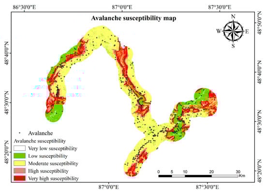
Figure 11.
Generated avalanche susceptibility map.
Figure 12 presents the spatial distribution of these susceptibility classes together with the corresponding avalanche samples. The results indicate extensive moderate-to-high susceptibility along the road network. LightGBM estimates that 18.15% of the study area falls in the very high class, 8.00% in high, 50.32% in moderate, 19.54% in low, and 3.99% in very low. Notably, about 76% of inventoried avalanche events occur within the moderate-or-higher classes, which supports the realism of the susceptibility map.
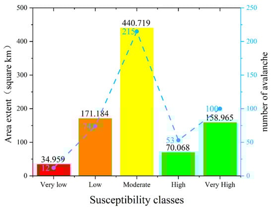
Figure 12.
Area and avalanche sample statistics of susceptibility levels.
Based on the spatial distribution of avalanche susceptibility predicted by the model, avalanches were found to be primarily concentrated along the midsection of the S232 route, particularly on both sides of the river valley, as well as the middle and lower sections of the X852 route. During the field investigation conducted throughout the 2023–2024 snow season, multiple avalanche events were identified around the scenic corridor. These events were all located in areas classified as high or very high susceptibility on the model-derived map, indicating a strong agreement between the evaluation results and actual conditions. Selected field-observed avalanche events are presented in Figure 13.
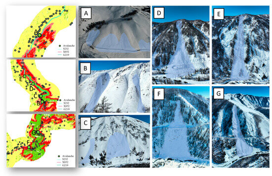
Figure 13.
Spatial distribution of avalanche susceptibility classes and field-verified avalanche locations. Panels (A–G) correspond to different representative road sections along the S232, X852, and G219 corridors.
In addition to the visual comparison, a spatial overlay analysis was conducted between the susceptibility map and field-recorded avalanche locations to quantitatively assess model reliability. The results showed that 76% of the mapped avalanche initiation zones fell within the moderate-to-very-high susceptibility classes. This spatial correspondence indicates a strong predictive agreement between the model and real-world avalanche occurrences.
Furthermore, field validation using UAV orthophotos and GPS-marked avalanche debris confirmed that the observed crown lines, deposition zones, and runout paths were accurately captured within the high-susceptibility belts predicted by the model. These belts are predominantly distributed along the middle sections of the S232 and X852 routes, coinciding with steep slopes (>30°) and areas of high TRI (>6), where dense snow accumulation and wind redistribution were observed during field campaigns.
Overall, the high spatial agreement between model predictions and observed avalanche paths demonstrates the practical validity of the proposed framework for identifying critical hazard zones and prioritizing monitoring and mitigation along mountain transportation corridors.
5. Discussion
5.1. Comparison with Previous Studies
The findings of this study are generally consistent with previous research on avalanche susceptibility modeling using machine learning. Similarly to Akay and Iban [26,27], our results confirm that ensemble tree-based algorithms, particularly LightGBM, achieve high predictive performance and robustness in complex alpine terrain. The identification of key conditioning factors such as slope, TRI, and wind speed also aligns with Maggioni et al. and Liu et al. [49,50], who emphasized the dominant role of topography and meteorological forcing in avalanche occurrence.
Beyond confirming these patterns, this study advances the literature by integrating SHAP-based explainable analysis to move from “which factors matter” to “how and where they matter.” Specifically, the SHAP dependence plots quantify nonlinear thresholds and pairwise interactions—for example, the slope peak around 30–40°, the TRI plateau near 5–7, and the wind-speed transition around 2.0–2.5 m s−1—thus linking model outputs to physically interpretable processes. Earlier ML work largely emphasized overall accuracy or global feature rankings; our approach complements those efforts by exposing factor response curves and interaction windows that are directly actionable for monitoring and early warning (e.g., prioritizing sensor placement on steep, high-relief, wind-exposed slopes).
Methodologically, we also complement studies that rely solely on statistical validation by incorporating independent field verification with UAV imagery and GPS-mapped events. The strong spatial agreement between mapped high-susceptibility zones and observed avalanches (≈76%) reinforces the operational reliability of explainable ML for hazard zoning in alpine transportation corridors. Taken together, these contributions position our framework as an incremental yet practical step from accurate prediction toward interpretable, site-aware decision support.
5.2. Thresholds and Interactions: Implications for Avalanche Monitoring and Early Warning
The SHAP dependence plots revealed several critical thresholds and interactions that provide valuable insights for avalanche monitoring and early warning in the Kanas Scenic Area transportation corridor.
First, terrain-related thresholds were clearly identified. Avalanches are most likely to occur on slopes between 30° and 40°, particularly when combined with high terrain ruggedness (TRI ≈ 5–7). These findings suggest that slope–ruggedness combinations can be prioritized for ground-based monitoring stations, drone inspections, or remote sensing surveillance. Second, climatic drivers demonstrated actionable thresholds. Maximum wind speed exhibited a transition zone around 2.0–2.3 m s−1, with susceptibility increasing rapidly before saturating above 2.5 m s−1. Such thresholds can be translated into real-time warning triggers using local meteorological stations, especially when high winds coincide with rugged terrain that favors snow redistribution. Third, vegetation and land-surface indicators provide additional guidance. Moderate vegetation cover (NDVI ≈ 0.65–0.75) was associated with peak susceptibility, whereas denser vegetation (>0.75) reduced instability. Monitoring NDVI changes via satellite or UAV imagery may therefore help detect areas where vegetation loss could amplify avalanche risk. Fourth, hydrological and microclimatic effects were evident. Areas within 0–2 km of river valleys exhibited the highest susceptibility, especially under warmer daily maximum temperatures. This highlights the importance of focusing patrols and structural mitigation measures along riverside road sections. Similarly, TWI values exceeding 7–8 showed a strong suppressive effect on avalanche probability, but this stabilizing role weakened in highly rugged terrain, suggesting that moisture can shift from protective to adverse under specific geomorphic conditions.
Overall, these thresholds and interactions extend the utility of ML-based susceptibility mapping by offering physically interpretable benchmarks for operational monitoring and early warning. Integrating such findings into local hazard management can support the development of threshold-based risk indices and adaptive alert systems, thereby enhancing preparedness for sudden avalanches in high-altitude transportation corridors.
5.3. Contributions, Limitations, and Future Directions
This study makes both scientific and practical contributions by integrating machine learning with explainable AI for avalanche susceptibility mapping in alpine transportation corridors. The use of SHAP enhanced model transparency and revealed the relative importance of topographic, climatic, and vegetation-related factors, thereby bridging data-driven modeling with physically interpretable mechanisms. These insights provide actionable guidance for disaster risk management: for instance, high TRI and steep slopes highlight zones requiring structural mitigation, while wind-exposed and sparsely vegetated slopes suggest the value of snow fences or reforestation programs. The strong agreement between predicted high-risk zones and observed avalanche events further validates the operational reliability of the framework, supporting its utility for proactive zoning and early warning in regions with limited monitoring infrastructure. Beyond the Kanas Scenic Area, the methodology offers a replicable template that balances predictive skill with interpretability, making it transferable to other alpine regions facing similar hazards.
Nevertheless, several limitations should be acknowledged. First, the reliance on ERA5-Land datasets introduces uncertainties, as its coarse resolution may miss micro-scale triggers such as short-lived gusts and localized snow redistribution, and prior studies have reported systematic biases in high-elevation terrain [51,52]. Second, despite its strong performance in the study area, transferability to other alpine regions with differing climate regimes, snowpack structures, or terrain types remains untested. Third, the current approach focuses on static susceptibility mapping, emphasizing spatial predisposition without accounting for the rapid temporal evolution of snowpack properties. Finally, while the SHAP framework enhances model transparency and factor ranking, it does not directly incorporate snow physical processes such as slab cohesion, weak layer evolution, or internal stress distribution. Coupling interpretable machine learning with process-based avalanche dynamics models may yield hybrid frameworks that balance accuracy, physical realism, and interpretability.
Future research should therefore prioritize three directions: expanding validation across multiple snow seasons and alpine regions to test robustness; incorporating higher-resolution meteorological and snowpack observations to refine environmental covariates; and combining interpretable ML with process-based models or real-time remote sensing indicators to enable spatiotemporal forecasting and dynamic early-warning systems. Pursuing these directions will support the development of more reliable, interpretable, and practically applicable avalanche forecasting tools for cold mountain regions.
6. Conclusions
This study proposes and validates an explainable ML framework for mapping snow avalanche susceptibility along the transportation corridor of the Kanas Scenic Area in the Altai Mountains, China. The main findings are as follows:
Among the five ML classifiers tested, Random Forest, XGBoost, LightGBM, Soft Voting and Stacking, LightGBM achieved the highest scores across all metrics (AUC = 0.9428, accuracy = 0.8681, F1-score = 0.8750, Cohen’s κ = 0.7366), indicating strong capability for delineating avalanche-prone zones and making it the preferred model for susceptibility mapping in this study.
Incorporating SHAP markedly improved model transparency. Global results identified TRI, MaxWind, slope, aspect, and NDVI as the dominant drivers. Dependence plots quantified actionable thresholds and interactions, including a TRI plateau at ~5–7, a slope peak at 30–40°, a MaxWind sign change at 2.0–2.3 m s−1 with saturation above 2.5 m s−1, a hump-shaped NDVI response with an optimum at 0.65–0.75, a near-river 0–2 km high-risk belt amplified by Tmax, and TWI suppression beyond 7–8 that is partially offset under high TRI. These interpretable patterns align predictions with physical processes and support corridor-scale risk mitigation.
Using LightGBM with 16 conditioning factors, we produced a susceptibility map classified by Jenks natural breaks into five classes: very high 18.15%, high 8.00%, moderate 50.32%, low 19.54%, and very low 3.99%. Spatial validation with 2023–2024 avalanche events shows that more than 75% of inventoried occurrences fall within the moderate-to-very-high classes, demonstrating the reliability of the map and its practical value for hazard zoning, infrastructure planning, and targeted risk reduction along high-elevation roads.
Limitations include reliance on reanalysis meteorology over complex terrain and a static mapping design. Future work will incorporate higher-resolution/downscaled forcings and event-time predictors, couple the data-driven outputs with physics-based avalanche dynamics for consequence mapping, and evaluate transferability via cross-region tests and spatial cross-validation with explicit uncertainty quantification. Overall, integrating remote sensing, ensemble ML, and explainable AI enhances the interpretability, accuracy, and usability of avalanche susceptibility assessment for cold region transportation corridors.
Author Contributions
Conceptualization, Y.L. and J.L.; methodology, Y.L., Z.Y. and J.L.; software, Y.L., Z.Y. and Q.C.; validation, Y.L.; formal analysis, Y.L. and J.L.; investigation, Y.L., Z.Y. and X.Q.; resources, Z.Y., Q.C. and J.L.; data curation, Z.Y. and Q.C.; writing—original draft, Y.L.; writing—review & editing, Z.Y. and Q.C.; supervision, Z.Y., Q.C. and J.L.; project administration, Q.C., X.Q. and J.L.; funding acquisition, Z.Y. and J.L. All authors have read and agreed to the published version of the manuscript.
Funding
This research was supported by the Key Technology Research and Development Program of Ministry of Transport of China (Grant No. 2022-ZD6-090); the Science and Technology Project for Transportation Industry of Xinjiang Transportation Department (Grant No. 2022-ZD-006); and the Research and Development Project of the Xinjiang Department of Science and Technology (Grant No. 2024B03042).
Data Availability Statement
The original contributions presented in the study are included in the article; further inquiries can be directed to the corresponding author.
Conflicts of Interest
Yaqun Li, Zhiwei Yang, Qiulian Cheng, Xiaowen Qiang and Jie Liu are employees of Xinjiang Transport Planning Survey and Design Institute Co., Ltd. The paper reflects the views of the scientists and not the company. The remaining authors declare that the research was conducted in the absence of any commercial or financial relationships that could be construed as a potential conflict of interest.
References
- Bhardwaj, A.; Sam, L. Reconstruction and characterisation of past and the most recent slope failure events at the 2021 rock-ice avalanche site in Chamoli, Indian Himalaya. Remote Sens. 2022, 14, 949. [Google Scholar] [CrossRef]
- McClung, D. Avalanche character and fatalities in the high mountains of Asia. Ann. Glaciol. 2016, 57, 114–118. [Google Scholar] [CrossRef]
- Mosavi, A.; Shirzadi, A.; Choubin, B.; Taromideh, F.; Hosseini, F.S.; Borji, M.; Shahabi, H.; Salvati, A.; Dineva, A.A. Towards an ensemble machine learning model of random subspace based functional tree classifier for snow avalanche susceptibility mapping. IEEE Access 2020, 8, 145968–145983. [Google Scholar] [CrossRef]
- Mott, R.; Vionnet, V.; Grünewald, T. The seasonal snow cover dynamics: Review on wind-driven coupling processes. Front. Earth Sci. 2018, 6, 197. [Google Scholar] [CrossRef]
- Schweizer, J.; Bruce Jamieson, J.; Schneebeli, M. Snow avalanche formation. Rev. Geophys. 2003, 41, 1016. [Google Scholar] [CrossRef]
- Leone, F.; Colas, A.; Garcin, Y.; Eckert, N.; Jomelli, V.; Gherardi, M. The snow avalanches risk on Alpine roads network. Assessment of impacts and mapping of accessibility loss. J. Alp. Res.|Rev. De Géographie Alp. 2014, 102. [Google Scholar] [CrossRef]
- Rafique, A.; Dasti, M.Y.; Ullah, B.; Awwad, F.A.; Ismail, E.A.; Saqib, Z.A. Snow avalanche hazard mapping using a GIS-based AHP approach: A case of glaciers in northern Pakistan from 2012 to 2022. Remote Sens. 2023, 15, 5375. [Google Scholar] [CrossRef]
- Eckert, N.; Corona, C.; Giacona, F.; Gaume, J.; Mayer, S.; van Herwijnen, A.; Hagenmuller, P.; Stoffel, M. Climate change impacts on snow avalanche activity and related risks. Nat. Rev. Earth Environ. 2024, 5, 369–389. [Google Scholar] [CrossRef]
- Haeberli, W.; Whiteman, C. Snow and ice-related hazards, risks, and disasters: Facing challenges of rapid change and long-term commitments. In Snow and Ice-Related Hazards, Risks, and Disasters; Elsevier: Amsterdam, The Netherlands, 2021; pp. 1–33. [Google Scholar] [CrossRef]
- Yariyan, P.; Omidvar, E.; Minaei, F.; Ali Abbaspour, R.; Tiefenbacher, J.P. An optimization on machine learning algorithms for mapping snow avalanche susceptibility. Nat. Hazards 2022, 111, 79–114. [Google Scholar] [CrossRef]
- Thakur, K.; Kumar, H. Avalanche susceptibility factors, trends, techniques, and practices in Indian Himalaya: A review. Earth-Sci. Rev. 2025, 269, 105207. [Google Scholar] [CrossRef]
- Fekete, A.; Tzavella, K.; Armas, I.; Binner, J.; Garschagen, M.; Giupponi, C.; Mojtahed, V.; Pettita, M.; Schneiderbauer, S.; Serre, D. Critical data source; tool or even infrastructure? Challenges of geographic information systems and remote sensing for disaster risk governance. ISPRS Int. J. Geo-Inf. 2015, 4, 1848–1869. [Google Scholar] [CrossRef]
- Statham, G.; Haegeli, P.; Greene, E.; Birkeland, K.; Israelson, C.; Tremper, B.; Stethem, C.; McMahon, B.; White, B.; Kelly, J. A conceptual model of avalanche hazard. Nat. Hazards 2018, 90, 663–691. [Google Scholar] [CrossRef]
- Bartelt, P.; Lehning, M. A physical SNOWPACK model for the Swiss avalanche warning: Part I: Numerical model. Cold Reg. Sci. Technol. 2002, 35, 123–145. [Google Scholar] [CrossRef]
- Christen, M.; Kowalski, J.; Bartelt, P. RAMMS: Numerical simulation of dense snow avalanches in three-dimensional terrain. Cold Reg. Sci. Technol. 2010, 63, 1–14. [Google Scholar] [CrossRef]
- Varol, N. Avalanche susceptibility mapping with the use of frequency ratio, fuzzy and classical analytical hierarchy process for Uzungol area, Turkey. Cold Reg. Sci. Technol. 2022, 194, 103439. [Google Scholar] [CrossRef]
- Durlević, U.; Valjarević, A.; Novković, I.; Vujović, F.; Josifov, N.; Krušić, J.; Komac, B.; Djekić, T.; Singh, S.K.; Jović, G. Universal snow avalanche modeling index based on SAFI–Flow-R approach in poorly-gauged regions. ISPRS Int. J. Geo-Inf. 2024, 13, 315. [Google Scholar] [CrossRef]
- Zheng, H.; Ding, M.; Huang, T.; He, Y.; Gao, Z.; Duan, Y. Integrating the frequency ratio and index of entropy with an extreme learning machine to map post-earthquake landslide susceptibility: A case study in Xingwen County, China. Stoch. Environ. Res. Risk Assess. 2024, 39, 4749–4771. [Google Scholar] [CrossRef]
- Pugliese Viloria, A.D.J.; Folini, A.; Carrion, D.; Brovelli, M.A. Hazard susceptibility mapping with machine and deep learning: A literature review. Remote Sens. 2024, 16, 3374. [Google Scholar] [CrossRef]
- Jomelli, V.; Delval, C.; Grancher, D.; Escande, S.; Brunstein, D.; Hetu, B.; Filion, L.; Pech, P. Probabilistic analysis of recent snow avalanche activity and weather in the French Alps. Cold Reg. Sci. Technol. 2007, 47, 180–192. [Google Scholar] [CrossRef]
- Pozdnoukhov, A.; Matasci, G.; Kanevski, M.; Purves, R.S. Spatio-temporal avalanche forecasting with Support Vector Machines. Nat. Hazards Earth Syst. Sci. 2011, 11, 367–382. [Google Scholar] [CrossRef]
- Choubin, B.; Borji, M.; Mosavi, A.; Sajedi-Hosseini, F.; Singh, V.P.; Shamshirband, S. Snow avalanche hazard prediction using machine learning methods. J. Hydrol. 2019, 577, 123929. [Google Scholar] [CrossRef]
- Choubin, B.; Borji, M.; Hosseini, F.S.; Mosavi, A.; Dineva, A.A. Mass wasting susceptibility assessment of snow avalanches using machine learning models. Sci. Rep. 2020, 10, 18363. [Google Scholar] [CrossRef]
- Mienye, I.D.; Sun, Y. A survey of ensemble learning: Concepts, algorithms, applications, and prospects. IEEE Access 2022, 10, 99129–99149. [Google Scholar] [CrossRef]
- Sakib, M.; Mustajab, S.; Alam, M. Ensemble deep learning techniques for time series analysis: A comprehensive review, applications, open issues, challenges, and future directions. Clust. Comput. 2025, 28, 73. [Google Scholar] [CrossRef]
- Akay, H. Spatial modeling of snow avalanche susceptibility using hybrid and ensemble machine learning techniques. Catena 2021, 206, 105524. [Google Scholar] [CrossRef]
- Iban, M.C.; Bilgilioglu, S.S. Snow avalanche susceptibility mapping using novel tree-based machine learning algorithms (XGBoost, NGBoost, and LightGBM) with eXplainable Artificial Intelligence (XAI) approach. Stoch. Environ. Res. Risk Assess. 2023, 37, 2243–2270. [Google Scholar] [CrossRef]
- Fang, Z.; Wang, Y.; Duan, G.; Peng, L. Landslide susceptibility mapping using rotation forest ensemble technique with different decision trees in the Three Gorges Reservoir area, China. Remote Sens. 2021, 13, 238. [Google Scholar] [CrossRef]
- Liu, B.; Guo, H.; Li, J.; Ke, X.; He, X. Application and interpretability of ensemble learning for landslide susceptibility mapping along the Three Gorges Reservoir area, China. Nat. Hazards 2024, 120, 4601–4632. [Google Scholar] [CrossRef]
- Choudhury, A.; Mondal, A.; Sarkar, S. Searches for the BSM scenarios at the LHC using decision tree-based machine learning algorithms: A comparative study and review of random forest, AdaBoost, XGBoost and LightGBM frameworks. Eur. Phys. J. Spec. Top. 2024, 233, 2425–2463. [Google Scholar] [CrossRef]
- Jabbar, H.G. Advanced threat detection using soft and hard voting techniques in ensemble learning. J. Robot. Control (JRC) 2024, 5, 1104–1116. [Google Scholar] [CrossRef]
- Chamola, V.; Hassija, V.; Sulthana, A.R.; Ghosh, D.; Dhingra, D.; Sikdar, B. A review of trustworthy and explainable artificial intelligence (XAI). IEEE Access 2023, 11, 78994–79015. [Google Scholar] [CrossRef]
- Li, M.; Sun, H.; Huang, Y.; Chen, H. Shapley value: From cooperative game to explainable artificial intelligence. Auton. Intell. Syst. 2024, 4, 2. [Google Scholar] [CrossRef]
- Kayhan, E.C.; Ekmekcioğlu, Ö. Coupling Different Machine Learning and Meta-Heuristic Optimization Techniques to Generate the Snow Avalanche Susceptibility Map in the French Alps. Water 2024, 16, 3247. [Google Scholar] [CrossRef]
- Ford, K.R.; Ettinger, A.K.; Lundquist, J.D.; Raleigh, M.S.; Hille Ris Lambers, J. Spatial heterogeneity in ecologically important climate variables at coarse and fine scales in a high-snow mountain landscape. PLoS ONE 2013, 8, e65008. [Google Scholar] [CrossRef]
- Nurakynov, S.; Sydyk, N.; Baygurin, Z.; Balakay, L. Advancements in Remote Sensing for Monitoring and Risk Assessment of Glacial Lake Outburst Floods. Geosciences 2025, 15, 211. [Google Scholar] [CrossRef]
- Yang, J.; Huang, X. 30 m annual land cover and its dynamics in China from 1990 to 2019. Earth Syst. Sci. Data Discuss. 2021, 13, 3907–3925. [Google Scholar] [CrossRef]
- Aranda, F.; Medina, D.; Castro, L.; Ossandón, Á.; Ovalle, R.; Flores, R.P.; Bolaño-Ortiz, T.R. Snow persistence and snow line elevation trends in a Snowmelt-Driven Basin in the Central Andes and their correlations with hydroclimatic variables. Remote Sens. 2023, 15, 5556. [Google Scholar] [CrossRef]
- Hao, J.-S.; Huang, F.-R.; Liu, Y.; Amobichukwu, C.A.; Li, L.-H. Avalanche activity and characteristics of its triggering factors in the western Tianshan Mountains, China. J. Mt. Sci. 2018, 15, 1397–1411. [Google Scholar] [CrossRef]
- Hao, J.; Li, L. Research progress and prospect of snow avalanche disaster prevention and control. J. Glaciol. Geocryol. 2022, 44, 762–770. [Google Scholar] [CrossRef]
- Wen, L.; Jia, J.; Yao, T. A review of study on snow avalanches monitoring. J. Glaciol. Geocryol. 2023, 45, 1679–1702. [Google Scholar] [CrossRef]
- Williams, C.; McNamara, J.; Chandler, D. Controls on the temporal and spatial variability of soil moisture in a mountainous landscape: The signature of snow and complex terrain. Hydrol. Earth Syst. Sci. 2009, 13, 1325–1336. [Google Scholar] [CrossRef]
- Zhuang, Y.; Xing, A.; Bilal, M.; Bartelt, P. The effect of ambient air temperature on meltwater production and flow dynamics in snow avalanches. Landslides 2024, 21, 2389–2398. [Google Scholar] [CrossRef]
- Thorn, C.E. The geomorphic role of snow. Ann. Assoc. Am. Geogr. 1978, 68, 414–425. [Google Scholar] [CrossRef]
- Fan, J.; Ma, X.; Wu, L.; Zhang, F.; Yu, X.; Zeng, W. Light Gradient Boosting Machine: An efficient soft computing model for estimating daily reference evapotranspiration with local and external meteorological data. Agric. Water Manag. 2019, 225, 105758. [Google Scholar] [CrossRef]
- Kutlug Sahin, E.; Colkesen, I. Performance analysis of advanced decision tree-based ensemble learning algorithms for landslide susceptibility mapping. Geocarto Int. 2021, 36, 1253–1275. [Google Scholar] [CrossRef]
- Lartey, B.; Homaifar, A.; Girma, A.; Karimoddini, A.; Opoku, D. XGBoost: A tree-based approach for traffic volume prediction. In Proceedings of the 2021 IEEE International Conference on Systems, Man, and Cybernetics (SMC), Melbourne, Australia, 17–20 October 2021; pp. 1280–1286. [Google Scholar]
- Nohara, Y.; Matsumoto, K.; Soejima, H.; Nakashima, N. Explanation of machine learning models using improved shapley additive explanation. In Proceedings of the 10th ACM International Conference on Bioinformatics, Computational Biology and Health Informatics, Niagara Falls, NY, USA, 7–10 September 2019; p. 546. [Google Scholar]
- Liu, J.; Zhang, T.; Hu, C.; Wang, B.; Yang, Z.; Sun, X.; Yao, S. A study on avalanche-triggering factors and activity characteristics in Aerxiangou, West Tianshan Mountains, China. Atmosphere 2023, 14, 1439. [Google Scholar] [CrossRef]
- Maggioni, M.; Gruber, U. The influence of topographic parameters on avalanche release dimension and frequency. Cold Reg. Sci. Technol. 2003, 37, 407–419. [Google Scholar] [CrossRef]
- Qian, L.; Zhao, P. Assessment of ERA5-Land Reanalysis Precipitation Data in the Qilian Mountains of China. Atmosphere 2025, 16, 826. [Google Scholar] [CrossRef]
- Zou, J.; Lu, N.; Jiang, H.; Qin, J.; Yao, L.; Xin, Y.; Su, F. Performance of air temperature from ERA5-Land reanalysis in coastal urban agglomeration of Southeast China. Sci. Total Environ. 2022, 828, 154459. [Google Scholar] [CrossRef]


Disclaimer/Publisher’s Note: The statements, opinions and data contained in all publications are solely those of the individual author(s) and contributor(s) and not of MDPI and/or the editor(s). MDPI and/or the editor(s) disclaim responsibility for any injury to people or property resulting from any ideas, methods, instructions or products referred to in the content. |
© 2025 by the authors. Licensee MDPI, Basel, Switzerland. This article is an open access article distributed under the terms and conditions of the Creative Commons Attribution (CC BY) license (https://creativecommons.org/licenses/by/4.0/).