Physics-Based Machine Learning for Vibration Mitigation by Open Buried Trenches

Featured Application

This work presents a novel and efficient Machine Learning (ML) methodology for the rapid prediction of Insertion Loss (IL) values for open trenches used in ground vibration mitigation. This approach serves as a compelling alternative to computationally intensive numerical methods like FEM or BEM. The developed ML models enable the rapid design optimization and real-time assessment of vibration barriers in geotechnical engineering. This is particularly useful for civil and geotechnical engineers aiming to mitigate vibrations from sources such as vehicles and construction operations, overcoming the significant computational costs and time constraints of traditional simulation methods.

Abstract

Mitigating ground vibrations from sources like vehicles and construction operations poses significant challenges, often relying on computationally intensive numerical methods such as Finite Element Methods (FEM) or Boundary Element Methods (BEM) for analysis. This study addresses these limitations by developing and evaluating Machine Learning (ML) methodologies for the rapid and accurate prediction of Insertion Loss (IL), a critical parameter for assessing the effectiveness of open trenches as vibration barriers. A comprehensive database was systematically generated through high-fidelity numerical simulations, capturing a wide range of geometric, elastic, and physical configurations of a stratified geotechnical system. Three distinct ML strategies—Artificial Neural Networks (ANN), Support Vector Machines (SVM), and Random Forests (RF)—were initially assessed for their predictive capabilities. Subsequently, a Meta-RF stacking ensemble model was developed, integrating the predictions of these base methods. Model performance was rigorously evaluated using complementary statistical metrics (RMSE, MAE, NMAE, R), substantiated by in-depth statistical analyses (normality tests, Bootstrap confidence intervals, Wilcoxon tests) and an analysis of input parameter sensitivity. The results clearly demonstrate the high efficacy of Machine Learning (ML) in accurately predicting IL across diverse, realistic scenarios. While all models performed strongly, the RF and the Meta-RF stacking ensemble models consistently emerged as the most robust and accurate predictors. They exhibited superior generalization capabilities and effectively mitigated the inherent biases found in the ANN and SVM models. This work is intended to function as a proof-of-concept and offers promising avenues for overcoming the significant computational costs associated with traditional simulation methods, thereby enabling rapid design optimization and real-time assessment of vibration mitigation measures in geotechnical engineering.

1. Introduction

The mitigation of vibrations resulting from the development of transportation networks (rail and road), activities in sectors such as construction and the exploration of geological resources, or even natural events like earthquakes, is a matter of great concern to society, particularly in densely populated urban environments [1]. These vibrations, depending on their source and distance, can cause discomfort to surrounding populations, significantly affecting the physiological and psychological aspects of human beings, as well as structural damage of varying importance to adjacent structures, or even failures in the operation of sensitive equipment [2,3,4,5]. Vibrations in the 1–80 Hz frequency range are perceptible to nearby residents, while higher-frequency vibrations, in the 16–250 Hz range, manifest as re-radiated noise inside buildings [3].

Two of the solutions considered effective to solve this problem involve the application of a finite geometric discontinuity (barrier), filled with some type of material that dissipates or promotes the reflection of incident energy (e.g., bentonite, cement-soil mixture, concrete, or geofoam), or open trenches. Vibrational energy propagates in the form of body waves (P and S waves) and surface waves (primarily Rayleigh waves) [6]. It is known that various factors, including the characteristics of the waves and the propagation medium, influence the performance of the barriers. The distance between the barrier and the vibration source also plays an important role in the filtering process. Çelebi et al. [7] concluded that passive isolation (barriers located further from the source) provides higher levels of isolation than active isolation (barriers near the source). To be effective, barriers must reflect, scatter, and diffract surface waves [4], since these types of vibrations, especially Rayleigh waves, carry most of the vibration energy over long distances [8].

While traditional numerical methods such as FEM or BEM are crucial for analyzing these complex systems, they often carry significant computational costs, especially for extensive parametric studies or real-time applications [2,6,9,10].

Our research delves into the efficacy of machine-learning-based vibration mitigation solutions. Open trenches serve as physical impediments, reducing seismic wave and vibration propagation through energy redirection or dissipation prior to reaching vulnerable structures [9]. Such a solution proves both effective and flexible, allowing for adaptation across varied geological and architectural settings. When compared to filled barriers, open trenches tend to exhibit greater efficacy in isolating vibrations caused by surface waves; however, their applicability is strongly conditioned by soil stability (they tend to require more maintenance) and geometry of the trench [7], also requiring the availability of space for installation. Woods [5] performed a series of scaled field experiments on vibration isolation by installing open trenches very close to the wave source as well as near the structure (or machine) to be protected. His research demonstrated that the ratio of the barrier’s depth to the wavelength of the Rayleigh wave (LR) is the most important geometric parameter in the process of damping wave propagation (he suggested that the depth of the barrier should be, at least, 0.6 LR, for effective vibration isolation). Other research [10,11,12,13] reached similar conclusions (this relationship should be around 0.7 LR or 0.8 LR, to ensure greater effectiveness in filtering vibrations), and that the depth of the trench is more decisive than its thickness [2]. The quantification of the effectiveness of implementing a trench can be achieved through the determination of the descriptor parameter “insertion loss” (IL), which indicates the difference in vibrational amplitude measured due to the insertion of a noise control device in a given system under study. Mathematically, insertion loss is defined as the logarithmic ratio of the vibrational velocity (in dB—decibel) before and after the insertion of this device [14], as demonstrated in the following equation (Equation (1)):

$$IL=20{\log }_{10}\left(\left|{\displaystyle \raisebox{1ex}{$V_{t1}$}\!\left/ \!\raisebox{-1ex}{$V_{t2}$}\right.}\right|\right)\mathrm{d}\mathrm{B}$$

(1)

Here, V_t1 represents the vibration velocity before the installation of the noise control device, and V_t2 represents the vibration velocity after its installation.

In this study, the application of different machine learning strategies—ANN, SVM, and RF—was motivated by their complementary characteristics in learning complex, non-linear mappings between input features (geometrical, physical, and elastic parameters) and insertion loss (IL) values across 11 frequency bands. Artificial neural networks (ANN) are particularly effective in approximating highly non-linear functions due to their layered structure and learning capacity. Support vector machines (SVM), on the other hand, perform well in high-dimensional spaces and are robust against overfitting in problems with limited training samples. Random forests (RF) offer interpretability and are less sensitive to parameter tuning, leveraging ensemble learning internally through decision tree aggregation. Each of these methods, however, presents specific biases or generalization limitations when employed individually. To address these shortcomings, an ensemble model was developed, synthesizing the predictions from the three approaches to enhance both accuracy and robustness. This ensemble acts as a meta-learner, effectively merging the distinct advantages of each method to provide a more stable and broadly applicable solution for predicting IL across various configurations.

Furthermore, recent advancements in data-driven methodologies have positioned machine learning (ML) as a potent alternative or valuable complement to conventional numerical techniques, particularly in engineering challenges characterized by intricate input–output relationships. Indeed, numerous studies have showcased ML’s capability for forecasting vibratory responses and other mechanical properties within geotechnical systems [15,16,17,18]. In the field of vibration mitigation, however, most studies remain centered on numerical simulations using FEM or BEM to analyze the performance of isolation measures [2,6,9,10]. Only a limited number of recent contributions have explored the integration of ML in this domain, such as using ANNs to predict vibration attenuation [16] or applying ensemble learning for structural response estimation [17,19].

This study is structured as follows: the Introduction outlines the current developments in the research area, highlighting key issues related to the problem and the methods used to address it; (i) the Numerical Method (FEM) Section explains its application in analyzing vibrational spectra through a model developed in MATLAB; (ii) the Machine Learning Section outlines the methodologies and theoretical foundations that sustain the main concepts of the research, subsequently presenting the results obtained from various algorithms, including artificial neural networks, support vector machines, random forests, and an ensemble stacking approach; and (iii) in the last section of this study, the conclusions are presented, highlighting the implications of the findings and suggesting areas for further research.

2. Numerical Method

The Finite Element Method (FEM) is a robust numerical technique widely employed in engineering to solve complex problems, particularly those involving structural dynamics and wave propagation [9,20,21,22,23,24,25]. This method discretizes a continuous domain into smaller, simpler elements (e.g., triangles in 2D, tetrahedrons or hexahedrons in 3D) connected at nodal points, where governing physical equations are approximated using interpolation functions to obtain an overall solution.

In this research, a FEM model was developed in MATLAB (version R2024b), based on the finite element model by Albino et al. [26]. The continuous domain was discretized using linear triangular elements. To ensure accurate results, a minimum of 8 elements per wavelength were considered, calculated for the S wave velocity and for the highest frequency of interest (160 Hz). Boundary conditions were handled by implementing absorbing layers along the lateral and bottom edges of the domain, which simulate non-reflecting boundaries with spatially varying damping based on an exponential profile [27], enabling gradual dissipation of seismic energy and avoiding artificial reflections.

While demanding significant computational resources, FEM’s capability is particularly powerful for solving wave propagation problems, modeling the interaction of mechanical waves with complex geometries, materials, and boundaries [22,28,29,30,31,32]. The method computes stiffness (K), mass (M), and damping (C) matrices, which describe the system. The time-dependent solution is often found using a time integration method, such as Newmark-beta or central difference, to calculate nodal displacements and velocities over time [9,21,22,24,25].

For each simulation, the fundamental material properties (Young’s Modulus, Poisson’s coefficient, and density) served as direct inputs for the FEM process, defining the elemental stiffness and mass matrices for the model. While the corresponding wave velocities (P-waves, S-waves, and Rayleigh waves) are derived from these properties and are conceptually important for aspects such as determining appropriate mesh sizing, they were not used as intermediate inputs in the simulation loop itself. The mesh represented a two-dimensional layered system with trench geometry. A damping coefficient was computed to simulate energy dissipation, with its spatial distribution dependent on the distance from the open trench. Vertical and horizontal displacements at specific surface receiver nodes were calculated to track wave propagation, and responses were analyzed in the frequency domain in one-third octave bands, providing insights about the effect of the open trench on the different frequencies. 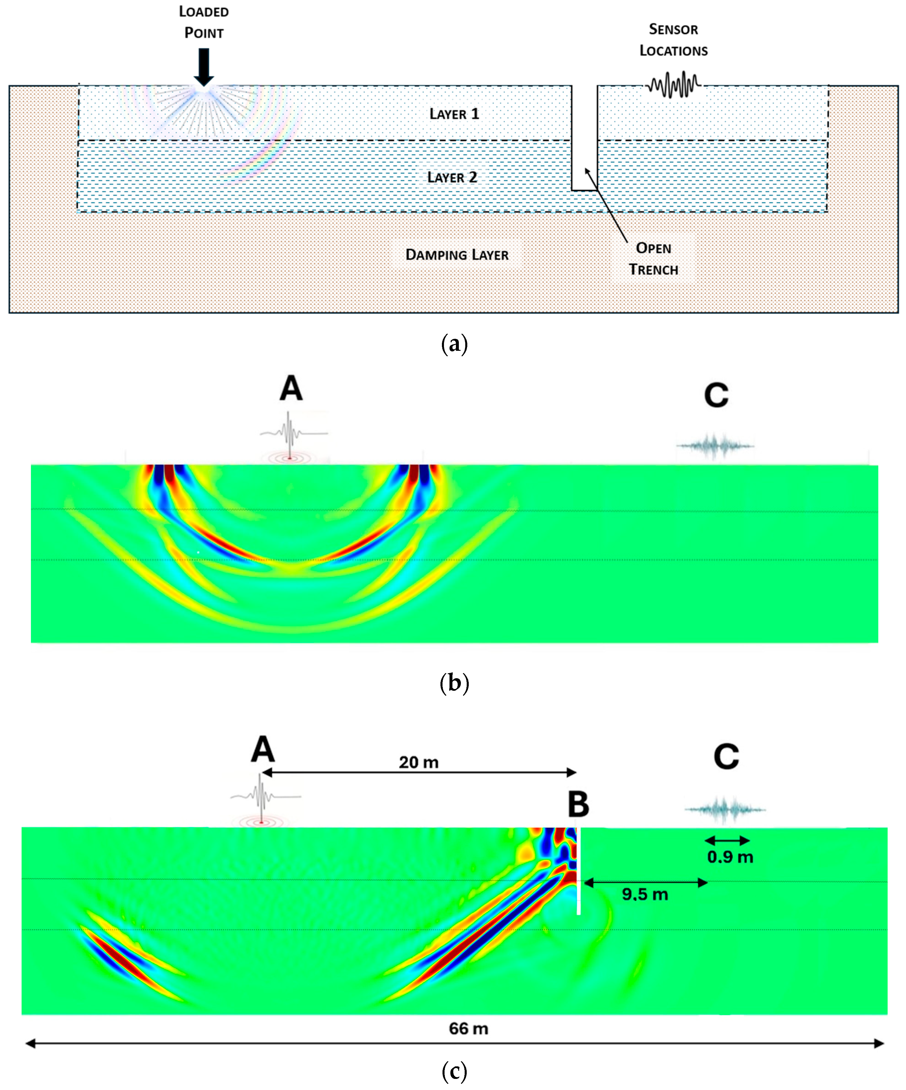Figure 1 illustrates an example of the model. It consists of two layers of homogeneous materials with variable thickness over a fixed 8 m damping layer (layers are delimited with dashed lines), measuring 66 m in length. The model was excited by a transient point load applied vertically to a single node on the domain’s surface (Ricker wavelet). This wavelet was generated with a center frequency (fc) of 75 Hz. Consequently, the magnitude of the applied force was not constant but varied over time according to the characteristic shape of the wavelet, which has a finite duration.

The impact point is 20 m to the left of the trench (which is 6 m deep and 0.36 m thick). Ten surface sensors recorded vibrational levels with and without the trench, positioned approximately 9.5 to 10.4 m to the right of the trench (with 10 cm spacing), as shown in Figure 1c. Figure 1b demonstrates an example of a simulation without the trench.

The thickness of the damping layer was kept fixed at 8 m, and a correlation was imposed between the values of the modulus of elasticity and density [33], according to (Equation (2)):

$$E=14.13{\gamma }_d-180.63$$

(2)

As already mentioned, all other parameters were varied randomly within known realistic limits (see

Table 1. Relevant parameters and limit variation ranges for the FEM simulation.

GEOMETRIC PARAMETERS
Parameter	Limit values
Thickness of layer 1	[1 to 5] m
Thickness of layer 2	[1 to 5] m
Depth of the trench	[3 to 7] m
Thickness of the trench	[0.1 to 0.5] m
ELASTIC PARAMETERS
Parameter	Limit values
Young modulus (E)	[10 to 150] MPa
Poisson coefficient (µ)	[0.27 to 0.37]
PHYSICAL PARAMETERS
Parameter	Limit values
Density (ρ)	[1350 to 2040] kg/m3

).

To ensure a representative exploration of the parameter space defined in Table 1, a uniform random sampling strategy was adopted. This approach enabled the generation of a diverse dataset by randomly selecting parameter combinations within their respective realistic bounds, without introducing bias or clustering effects. Although simple to implement, uniform random sampling provides sufficient variability and coverage in multidimensional spaces, making it suitable for the generation of synthetic datasets for machine learning purposes. This ensured that the trained models were exposed to a wide range of plausible physical and geometrical configurations, enhancing their ability to generalize to unseen cases.

3. Machine Learning

In recent decades (starting in the 1960s of the 20th century), artificial intelligence (AI) has assumed a significant role in human society, mainly through the application of machine learning (ML) methodologies to an increasing number of aspects of our daily lives. The success of these ML methods is so universal that it is, since the 1990s, recognized as the most successful branch of AI. The development of technology and computer infrastructure has enhanced the usability of ML methodologies in solving complex problems. ML algorithms can harness the growing volume of data now easily available in online databases to improve accuracy and predictive power by identifying complex patterns, refining models with diverse inputs, and continuously learning from new information. This can reduce the necessity of traditional approaches such as empirical trial and error. People interact with AI in nearly every aspect of human society, from voice and facial recognition to traffic and weather alerts, medical diagnostics, autonomous vehicles, optimizing production lines, and predicting material properties [16,18,34].

The use of machine learning in this context is particularly justified by the high computational cost and limited scalability of traditional numerical methods such as FEM or BEM. While these methods provide accurate physical insight, they require long simulation times for each configuration, especially when exploring wide parametric spaces involving geometrical and mechanical variations. Machine learning offers a data-driven alternative capable of learning complex, non-linear relationships from simulation results, allowing for rapid predictions of insertion loss (IL) across a wide range of configurations without rerunning computationally expensive simulations. This approach enables real-time applications, parametric optimization, and design sensitivity studies, which would otherwise be impractical using conventional methods alone.

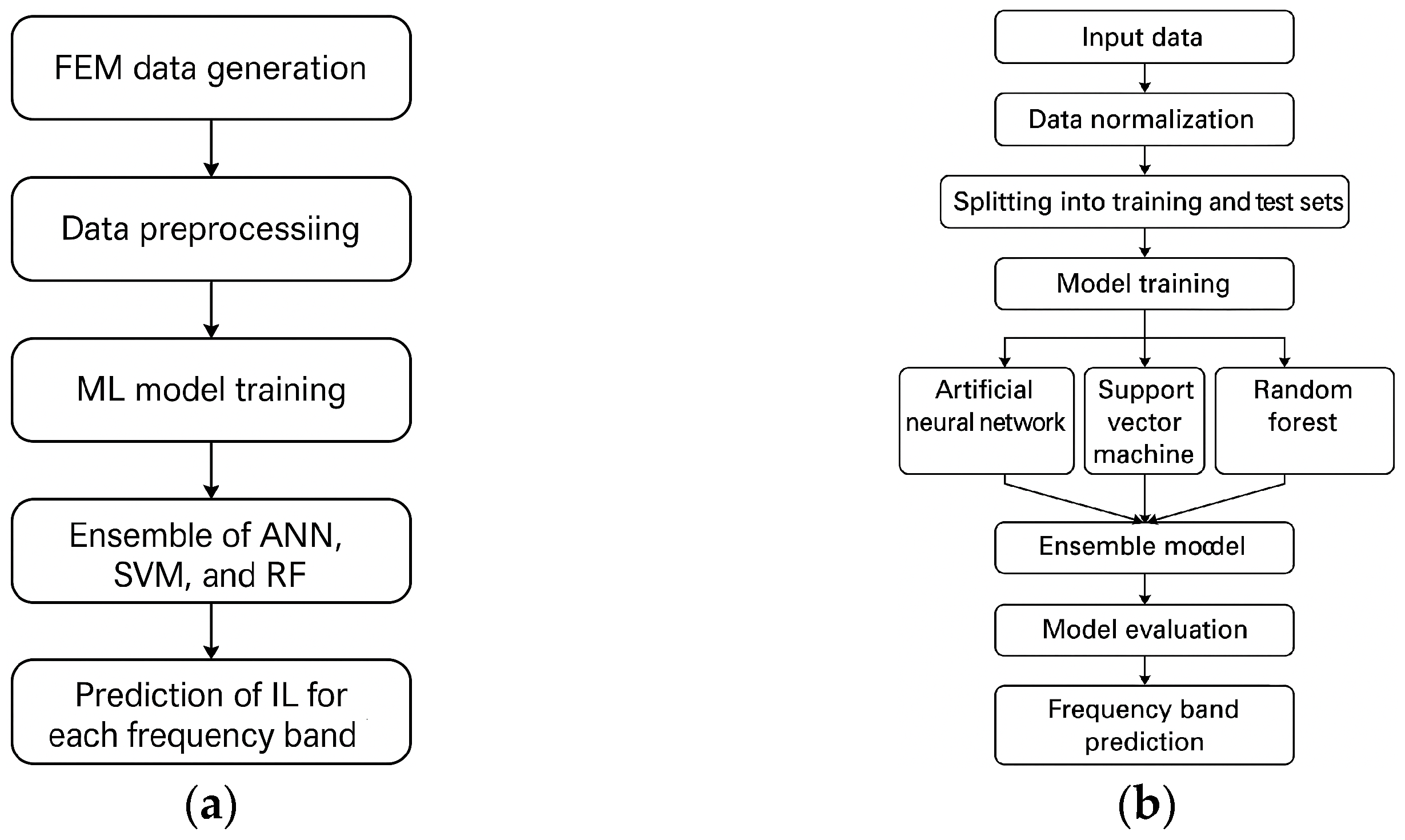
The workflow followed in this study for the application of machine learning algorithms is outlined in Figure 2a. The same procedure was applied independently to three different models: Artificial Neural Networks (ANN), Support Vector Machines (SVM), and Random Forests (RF). Each model was trained using the same set of input features and target values, and their performances were evaluated separately before combining their predictions in an ensemble model. The input parameter set for the machine learning models was carefully selected to include ten primary geometric and material properties: the thicknesses of both layers (h_lay1 and h_lay2), the depth and thickness of the open trench (h_trench and t_trench respectively), the Young’s Modulus, the density and Poisson coefficient of both layers (E₁, E₂, $\rho$₁, $\rho$₂, ν₁, and ν₂ respectively). A more detailed schematic of the modeling process—including preprocessing, training, evaluation, and sensitivity analysis is presented in Figure 2b. This unified approach ensures methodological consistency across all models and facilitates direct comparison.

A standardized data preparation strategy was employed. The complete dataset was first partitioned into a training set (70%), used for the k-fold cross-validation process, and a final hold-out validation set (15%). The remaining 15% of the data was used for testing within the cross-validation folds. Crucially, to prevent data leakage, data normalization (z-score) was applied independently within each cross-validation fold. The normalization parameters (mean and standard deviation) were learned solely from each fold’s training data and then applied to its corresponding test set and to the global validation set. This robust approach ensures that model evaluation is unbiased and accurately reflects performance on truly unseen data [35]. No outlier removal was conducted, as the dataset did not exhibit anomalous values that would justify exclusion. Subsequently, a systematic and reproducible approach was employed for hyperparameter tuning for all machine learning models (ANN, SVM, RF, and the Meta-RF). The methodology was based on a nested cross-validation framework. The outer loop (k = 15 folds) was dedicated to providing an unbiased evaluation of the final model performance. Within each of these outer folds, an inner cross-validation loop (k = 5 folds) was used as the objective function for a Bayesian Optimization algorithm. This algorithm systematically searched the predefined hyperparameter space for the configuration that minimized the cross-validated Root Mean Square Error (RMSE) on the inner folds. This ensures that the hyperparameter tuning for each outer fold was performed on data completely independent of its test set, thus avoiding any optimistic bias. The final, optimized configurations reported for each model are therefore the result of this rigorous and automated search process.

Table 2. Hyperparameters applied in each ML model. Note: RF is mentioned as an individual model here, although it is, per se, a combination of several decision trees).

MODEL	HYPERPARAMETERS
ANN	Training function: trainbr (Bayesian Regularization) Hidden layers: 2 layers, with the number of neurons optimized via BayesOpt in each fold (search range: [10, 30] for each layer). Activation function: logsig (for all hidden layers) Learning rate (fixed): 0.05 Regularization parameter (mu): Optimized via BayesOpt in each fold (search range: [10−4, 10−1]) mu_dec: 0.1 mu_inc: 2 mu_max: 1010 Maximum validation failures: 200 Minimum gradient: 10−9 Epochs: 500 Cross-validation folds: Nested (Outer: 15 folds; Inner: 5 folds)
SVM	Kernel: Gaussian Standardize (Normalization): Applied manually before training (z-score), and disabled in the function (‘Standardize’, false). Hyperparameter tuning: Bayesian Optimization (bayesopt) in each outer fold.
	Optimized Hyperparameters: BoxConstraint (C): (logarithmic search range: [10−5, 105]) KernelScale: (logarithmic search range: [10−5, 105]) Epsilon: (logarithmic search range: [10−6, 10−0.5])
	Optimization method: Bayesian expected-improvement-plus with 40 evaluations per fold. Cross-Validation: Nested (Outer: 15 folds; Inner: 5 folds)
RF	Method: Bag (Bootstrap Aggregating) Learner: Decisions Trees Hyperparameter Tuning: Bayesian Optimization (bayesopt) in each outer fold. Optimized Hyperparameters:
	NumLearningCycles (Number of trees): (search range: [50, 500]) MinLeafSize (Minimum leaf size): (search range: [1, 20]) NumVariablesToSample (Number of predictors to sample): (search range: [1, 10])
	Optimization Method: expected-improvement-plus with 30 evaluations per fold. Cross-Validation: Nested (Outer: 15 folds, Inner: 5 folds)
Meta-RF (with feature stacking)	Meta-Model: Random Forest Regressor (fitrensemble with ‘Method’, ‘Bag’). Input (Features): Enriched stacking, combining: the predictions from the 3 base models (ANN, SVM, RF, – 3 × 11 = 33 features) and the 10 original physical features (total: 43 features). Preprocessing: Z-score normalization applied to the full set of 43 features. Hyperparameter Tuning: Bayesian Optimization (bayesopt) in each outer fold.
	Optimized Hyperparameters: NumLearningCycles (Number of trees): (search range: [50, 500]) MinLeafSize (Minimum leaf size): (search range: [1, 20]) NumPredictorsToSample (Number of predictors to sample): (search range: [5, 43])
	Optimization Method: expected-improvement-plus with 40 evaluations per fold. Cross-Validation: Nested (Outer: 15 folds, Inner: 5 folds)

shows these optimal hyperparameters applied in each ML model.

The performance of all the predictive models contemplated in this study was evaluated using four complementary statistical metrics: RMSE, MAE, NMAE, and the correlation coefficient (R). The Root Mean Squared Error (RMSE) quantifies the average magnitude of the prediction error in decibels (dB), placing greater emphasis on larger deviations due to its quadratic formulation (see Equation (3)) [36]. Lower RMSE values indicate higher predictive accuracy by showing how closely the predicted insertion loss (IL) aligns with the numerical (target) IL across the datasets.

$$RMSE=\sqrt{\sum _{i=1}^n{\displaystyle \frac{{({\hat{y}}_i-y_i)}^2}{n}}}$$

(3)

with $n$ being the number of observations, ${\hat{y}}_i$ being the predicted values, and $y_i$ the numerical values, in this situation [37]. In contrast, the Mean Absolute Error (MAE) measures the average of the absolute differences between predicted and true IL values, also expressed in dB [38].

Unlike RMSE, MAE penalizes all errors equally, offering a more interpretable measure of typical prediction deviations and providing a general sense of model accuracy (Equation (4)).

$$MAE={\displaystyle \frac{1}{n}}\sum _{i=1}^n\left|y_i-{\widehat{y}}_i\right|$$

(4)

with $n$ being the number of observations, $n$ being the predicted values, and $y_i$ the numerical values.

To enable comparison across datasets with different scales, the Normalized Mean Absolute Error (NMAE) is employed, which represents the MAE normalized by the range of the true IL values [39]. Being dimensionless, NMAE facilitates an assessment of the relative error magnitude, with lower values indicating higher reliability of the model (Equation (5)).

$$NMAE={\displaystyle \frac{MAE}{\max \left(y\right)-\mathrm{m}\mathrm{i}\mathrm{n}\left(y\right)}}$$

(5)

where $\max \left(y\right)$ and $\min \left(y\right)$ represent the maximum and minimum of the numerical values, respectively.

Lastly, the Pearson correlation coefficient (R) evaluates the linear association between predicted and numerical IL values, with values close to 1 denoting a strong positive correlation [40]. This metric reflects the model’s ability to capture the overall trends in the data (see Equation (6)).

$$R={\displaystyle \frac{\sum _{i=1}^N(x_i-\overline{x})(y_i-\overline{y})}{\sqrt{{\sum _{i=1}^N(x_i-\overline{x})}^2}\sqrt{{\sum _{i=1}^N(y_i-\overline{y})}^2}}}$$

(6)

In Equation (6), $N$ is the number of paired observations in the dataset, $x_i$ and $y_i$ are the individual sample points from the two variables, and $x$ and $y$ are the means of the variables. Together, these metrics offer a robust and multidimensional perspective on the model’s predictive performance, balancing absolute error quantification with trend fidelity.

To ensure statistical robustness and interpretability of the results, three complementary analyses were introduced: (i) normality assessment of the performance metrics, (ii) bootstrap confidence intervals, and (iii) paired statistical testing.

First, the Shapiro–Wilk test was applied to the distribution of performance metric values (RMSE, MAE, NMAE and R) across cross-validation folds, which is fundamental for understanding their statistical properties and guiding the choice of subsequent inferential methods (Equation (7)).

$$W={\displaystyle \frac{{\left({\sum }_{i=1}^n{a}_i{x}_{\left(i\right)}\right)}^2}{{\sum }_{i=1}^n{(x_i-\overline{x})}^2}}$$

(7)

where $x_{\left(i\right)}$ are the ordered sample values, $\overline{x}$ is the sample mean, and $a_i$ are the coefficients derived from the expected values and covariance matrix of the normal distribution. The Shapiro–Wilk method is particularly powerful and well-suited for small to moderate sample sizes [41].

Secondly, bootstrap resampling with replacement was employed to estimate 95% confidence intervals for the RMSE, MAE, NMAE and R metrics, thus quantifying the uncertainty and reliability of each model’s performance [42] (Equation (8)).

$${\mathrm{C}\mathrm{I}}_{(1-\mathsf{\alpha })}=\left[{\mathsf{\theta }}_{\mathsf{\alpha }/2}^{\mathrm{*}},{\mathsf{\theta }}_{1-\mathsf{\alpha }/2}^{\mathrm{*}}\right]$$

(8)

where ${\mathsf{\theta }}_{\mathsf{\alpha }/2}^{\mathrm{*}}$ and ${\mathsf{\theta }}_{1-\mathsf{\alpha }/2}^{\mathrm{*}}$ are the percentile bounds (e.g., 2.5th and 97.5th percentiles for 95% CI).

Finally, Wilcoxon signed-rank tests were applied to determine whether differences in model performance across the training, test, and validation sets were statistically significant. This non-parametric test is fundamental for assessing potential overfitting and validating the model’s generalization capability, especially when the assumption of normality or symmetry of differences cannot be met. It evaluates the null hypothesis that the median of the differences between paired observations is zero (Equation (9)).

$$T=\sum _{i=1}^{N}sgn\left(d_i\right)·R_i$$

(9)

where $d_i$ is the difference between paired values, $sgn\left(d_i\right)$ is the sign of that difference, $R_i$ is the rank of the absolute difference ∣$d_i$∣ and $N$ is the number of pairs (e.g., the number of cross-validation folds). The combined application of these three techniques reinforces the statistical validity of the model comparison and supports robust conclusions regarding predictive performance and model generalization [43].

3.1. Artificial Neural Networks

An Artificial Neural Network (ANN) is a mathematical model that simulates the structure and functional aspects of biological neural networks. An ANN is, nowadays, a powerful tool for modeling complex non-linear relationships between dependent and independent variables, operating without relying on prior assumptions or existing mathematical frameworks. This methodology consists of a set (usually a large number) of interconnected non-linear computational elements, called artificial neurons, that process information through a connectionist approach. The structure of the ANN is modified based on the data that traverse the network during the learning or training phase. If successfully trained, the resulting model will be able to preview response variables in the presence of new input parameters. ANNs can be divided into three main groups: supervised, unsupervised, and semi-supervised learning networks. Under the supervised scope, regression (or function approximation) ANNs attempt to learn and then generalize the non-linear relations between the independent and dependent variables [15,44]. This methodology is widely used in the engineering field, for example, in non-destructive testing to monitor structures. It is also applied in pathology assessment, landslide risk evaluation, and monitoring of cracks in built structures, as well as predicting relevant mechanical and physical parameters, thereby reducing the need for laboratory or field tests [17,45,46,47].

Figure 3 illustrates the process of a supervised artificial neural network with backpropagation.

In this study, a supervised regression ANN model was developed in MATLAB to predict the parameter “insertion loss—IL”. The dataset was partitioned for training, testing, and validation, with the commonly used percentages of 70%, 15%, and 15%, respectively [35]. Instead of a fixed architecture, the model’s key hyperparameters—including the number of neurons in its two hidden layers—were systematically optimized using the Bayesian Optimization algorithm within the nested cross-validation framework previously described (see Table 2). The training algorithm used was trainbr, which updates the weights and biases based on Levenberg–Marquardt optimization with Bayesian regularization to produce a network that generalizes well. Additionally, the logsig activation function (logistic sigmoid) was used between each layer. This activation function was considered advantageous as its inherent output bounding facilitates the ANN’s learning process, especially when working with normalized input parameters. For further information about the Bayesian regularization backpropagation network training function (trainbr) and the logsig activation function, refer to [45].

Sensitivity analysis of the artificial neural network model was conducted to assess the influence of each input parameter on the predicted insertion loss. A perturbation-based global approach was applied, whereby each input variable was individually increased by 5% while the remaining variables were held constant. The trained ANN was then used to compute the change in predicted output resulting from this modification. This process was repeated for each of the neural networks trained during the 15-fold cross-validation, and the mean absolute change in output was recorded for each input variable. The average sensitivity across folds was normalized to yield a relative importance score for each parameter, expressed as a percentage. The standard deviation across folds was also computed to indicate the variability of each input’s influence. This method allows the identification of the most influential physical parameters on the predicted insertion loss, thus enhancing the interpretability of the model and providing useful guidance for future design and optimization.

3.2. Support Vector Machines

Support Vector Machines (SVM) is a widely used ML technique since the work of Boser et al. [48,49,50], which introduced it for classification problems. During that decade, it rapidly evolved and expanded its application scope, being nowadays applied in both classification and regression tasks, due to its accuracy and simplicity. The main concept in this algorithm is to find a way to separate groups of data features (vectors), finding an optimal separating hyperplane with the maximum distance between support vectors of the groups of data features. The data points located on the periphery of the data group are designated support vectors and influence the position and orientation of the hyperplane [18]. SVMs are effective even with small training datasets, though non-linear factors may be required to separate points that cannot be divided by a simple hyperplane, a process known as Kernel machines [18,48,49]. 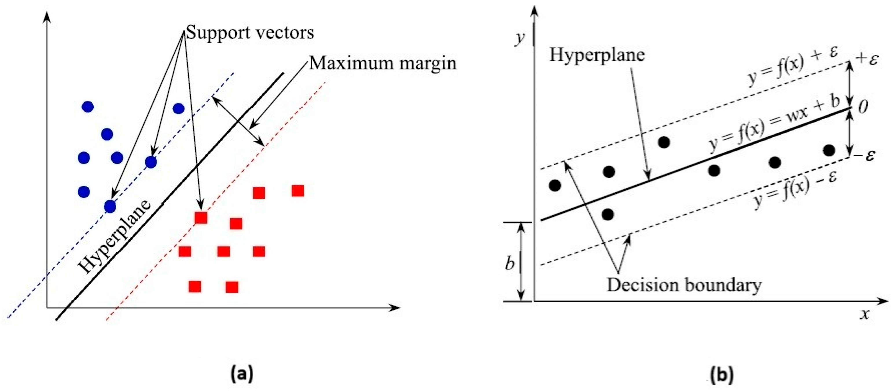Figure 4 shows a diagram representing a SVM for classification and regression.

In this study, a support vector regression (sometimes designated as SVR) model was developed and trained in the MATLAB environment to predict the same parameter (IL). This SVM algorithm aims at identifying a function that approximates the data while remaining within a margin of tolerance. The optimal solution is a hyperplane that maximizes the number of data points falling within a specified error limit. In most practical scenarios, data cannot be perfectly separated by a straight line or hyperplane. To address this, a penalty parameter and a kernel function are used. The penalty parameter allows for some misclassification by balancing the goal of maximizing the margin between data classes and minimizing the total distance of misclassified points. This approach, called the “soft margin,” ensures the margin is wide enough to correctly classify most of the data. Kernel functions, on the other hand, implicitly transform the original data (when it is impossible to separate it linearly) into a new feature space where it becomes linearly separable (this is known as the Kernel trick). Common kernel functions include linear, polynomial, Gaussian, and sigmoid expressions [51]. The “fitrsvm” training function was selected, and the SVM model used a Gaussian radial basis function (Gaussian kernel), which allowed the algorithm to handle non-linear relationships between the features and IL values [52]. Crucially, the model’s key hyperparameters, such as the BoxConstraint, KernelScale, and Epsilon, were not manually set but were systematically determined for each cross-validation fold using the Bayesian Optimization framework detailed in Table 2. The Gaussian radial basis function ($\phi \left(x\right)$) is given by (Equation (10)):

$$\phi (x)=e^{-{\displaystyle \frac{{\left|\left|x-u_j\right|\right|}^2}{2{\sigma }^2}}}$$

(10)

with $\left|x-u_j\right|$ being the Euclidian (absolute) distance between an input vector $x$ in the input space and $u_j$ (the support vectors, those specific data points from the dataset that will define the decision boundary of the SVM model), and ${\sigma }^2$ is the variance (also called kernel scale). Large variances result in wider Gaussian curves, meaning the influence of the support vectors spreads out over the input space. The opposite means that the influence of the support vectors is more localized. In these basis functions, the normalization coefficient is unimportant, since all the functions (for each value of $x$) will be affected by the tuned $w_j$ parameters of the non-linear function (Equation (11)), to determine the predicted output ($y(x,w)$):

$$y(x,w)=\sum _{j=1}^{M-1}{w}_j\phi (x)$$

(11)

where $\mathrm{w}$ is the collective representation of all the $w_j$ coefficients, and $M$ is the number of support vectors used in the model.

To evaluate the relative influence of each input parameter on the predicted insertion loss, a sensitivity analysis was conducted for the support vector machine (SVM) model. The approach consisted in perturbing each input variable individually by +5% while keeping all other variables constant and computing the corresponding variation in the predicted outputs. This procedure was applied across the 15 folds of the cross-validation, using the models trained for each fold and each frequency band. For each fold, the absolute difference between the original predictions and the perturbed ones was calculated and averaged across all training observations and output frequencies. This yielded a sensitivity score for each input variable per fold. The final importance of each variable was obtained by averaging these sensitivity scores across folds and normalizing the results to express relative importance in percentage terms. The standard deviation was also computed to reflect the uncertainty associated with each variable’s influence.

3.3. Random Forests

Random Forests (RF) is a supervised learning algorithm that employs decision trees (DT) as its base weak learners (the methods that have, per se, a poor predictive capacity). It should be noted that RF is not a single-model technique, but rather an ensemble learning method, in which multiple decision trees are trained and aggregated to produce a collective prediction. Each one of the DT’s that composes the RF model is generated slightly differently [52]. This algorithm constructs decision trees using the bagging method, which involves parallel training. The core concept is to create a collection of individual decision trees by randomly selecting subsets of features—hence the term “Random Forest”. After the decision trees are built, their outputs are combined through majority voting in classification tasks or averaging in regression tasks (it is possible to apply any other criteria suitable to a specific purpose). This approach enhances predictive performance by leveraging the diversity of the trees, leading to more robust and accurate results, reducing the risk of overfitting problems [18,19,53,54,55]. 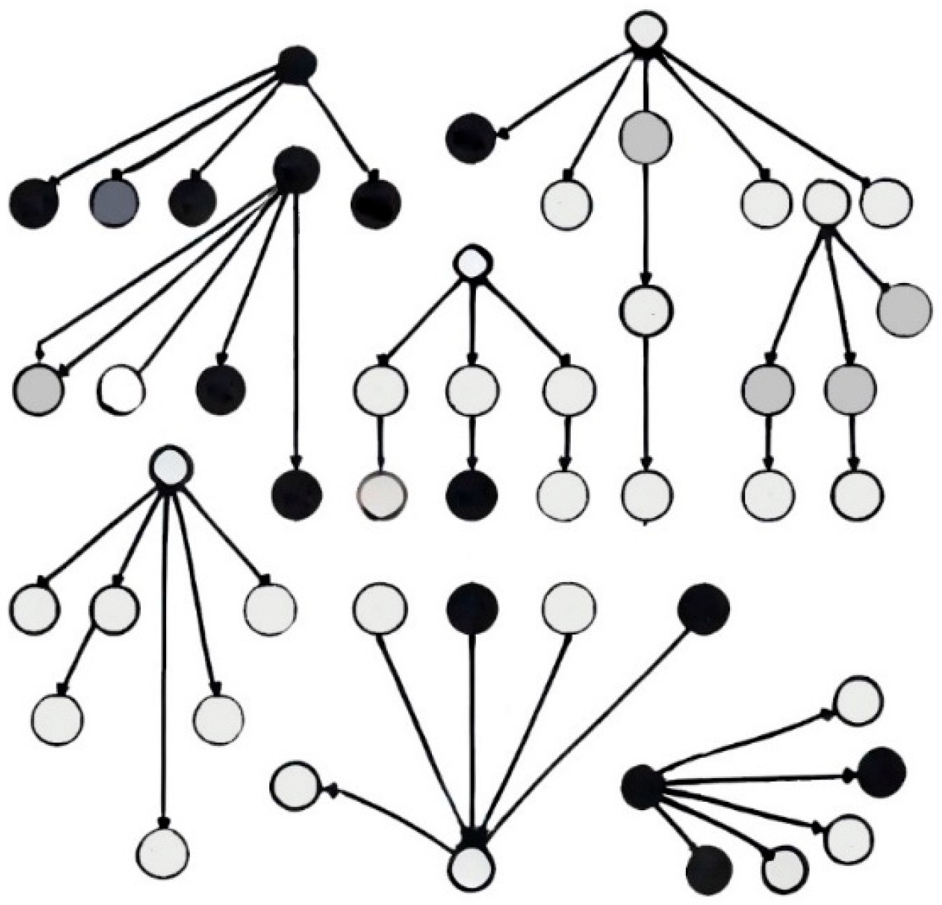Figure 5 represents a RF diagram, with several decision trees, each one of them with a random and different number of features and composed also by a random subset of data (thus the designation random forest, because it is made of several decision trees, with multiple sources of randomness).

In this study, a MATLAB script applying a Random Forest (RF) algorithm was developed to predict 11 target outputs (one for each frequency band). The model was constructed as an ensemble of decision trees using the bagging (bootstrap aggregation) method. In line with the robust methodology applied to all models, the key hyperparameters—such as the number of learning cycles (trees), the minimum leaf size, and the number of variables to sample—were not predefined. Instead, they were systematically tuned for each cross-validation fold via the Bayesian Optimization framework described in Table 2. The collective prediction of the RF is the average output from all individual trees in the ensemble, represented mathematically as (Equation (12)):

$$\widehat{\mathrm{y}}={\displaystyle \frac{1}{\mathrm{K}}}\sum _{\mathrm{k}=1}^{\mathrm{K}}{\mathrm{T}}_{\mathrm{k}}\left(\mathrm{X}\right)$$

(12)

where $\widehat{\mathrm{y}}$ is the predicted output, $\mathrm{K}$ the total number of decision trees of the RF model, and ${\mathrm{T}}_{\mathrm{k}}\left(\mathrm{X}\right)$ is the prediction of the $\mathrm{k}$-th tree for the input data $\mathrm{X}$. Predictions were generated for the training, testing, and validation sets.

A perturbation-based sensitivity analysis was carried out to assess the influence of each input parameter on the predictions of the Random Forest model. For each fold of the cross-validation procedure, a +5% variation was applied individually to each input feature, while keeping the remaining variables unchanged. The model’s response to the perturbed inputs was compared with the original predictions, and the absolute differences were computed for all output frequencies. This process was repeated across all folds, and the average variation induced by each input was calculated. The relative importance of each input parameter was then expressed as a percentage of the total variation. The results were summarized in a bar chart displaying the mean sensitivity values, allowing a clear identification of the most influential features in the prediction of insertion loss.

3.4. Ensemble Stacking Model

Ensemble models in ML combine several individual models to improve prediction accuracy, robustness, and generalization compared to single-model approaches. The underlying principle is that individual models may capture different aspects of the data or learn from different features, leading to diverse perspectives on the same prediction task. When combined, their collective insights tend to outperform any individual model in terms of overall performance [56]. In many real-world applications, including acoustic predictions like the IL data patterns are often complex and involve non-linear relationships. Single models such as ANNs, SVMs, or RFs may have inherent limitations in capturing all the nuances of the data due to biases from their individual learning architectures. An ensemble model mitigates these weaknesses by averaging or integrating the predictions of several individual models, leading to reduced variance and bias, and increased stability, which means the predictions become less sensitive to variations [57].

In this research, a MATLAB script was designed to implement an ensemble model for predicting IL, specifically termed “Meta-Random Forest (Meta-RF)”. This meta-model leverages the individual predictions generated by the ANN, SVM, and RF base models. The Meta-RF model employed a multi-stage approach to combine these base predictions. Initially, for each observation and each cross-validation fold, the raw predictions from the three base models (ANN, SVM, and RF) were aggregated. These aggregated raw predictions collectively formed the input features for the meta-model, aiming to provide a rich and detailed view of each base predictor’s output without simplifying it to mere summary statistics. This can be conceptualized as (Equation (13)):

$$X_{meta-raw}=\left[{Pred}_{ANN},{Pred}_{SVM},{Pred}_{RF}\right]$$

(13)

where ${Pred}_{ANN}$, ${Pred}_{SVM}$, and ${Pred}_{RF}$ were the raw prediction matrices from the respective base models, concatenated horizontally to form the raw input feature matrix for the meta-model.

To standardize the scale of these newly generated features and facilitate stable model training, a z-score normalization was applied. This transformed the raw features to have a mean of zero and a standard deviation of one (Equation (14)):

$$X_{norm}={\displaystyle \frac{X_{raw}-\mu }{\sigma }}$$

(14)

where $\mu$ is the mean and $\sigma$ is the standard deviation computed from the training data for each feature.

The input feature space for the meta-learner was constructed using an enriched stacking approach. It combines the predictions from the three base models across all 11 frequency bands (3 models × 11 bands = 33 features) with the 10 original, primary physical properties. This results in a comprehensive 43-dimensional feature set designed to provide the meta-learner with both the learned abstractions of the base models and the raw underlying physical context. Prior to training, this combined feature set was normalized using a standard z-score transformation. Notably, dimensionality reduction techniques such as PCA were intentionally omitted in the final methodology, as the feature space was deemed manageable and initial tests did not show a clear benefit that would outweigh the loss of interpretability.

Finally, a Random Forest (RF) model for regression (fitrensemble in MATLAB with ‘Method’, ‘Bag’) was trained directly on these 43 normalized features. The hyperparameters for this meta-learner were not predefined but were systematically tuned using the same nested Bayesian Optimization framework applied to the base models. Within each outer cross-validation fold, the optimization algorithm searched for the ideal combination of key hyperparameters, including the number of trees (NumLearningCycles, in the range [50, 500]), the minimum leaf size (MinLeafSize, in the range [1, 20]), and the number of predictors to sample at each split (NumVariablesToSample, in the range [5, 44]). This process ensures that the Meta-RF itself is optimally configured for the specific training data within each fold, maximizing its ability to model complex, non-linear relationships in the combined feature set. As with the individual models, the performance of this Meta-RF ensemble was evaluated by computing standard metrics such as RMSE, MAE, NMAE and R across the training, test, and validation sets.

The results achieved by this method are then compared with the other three approaches (ANN, SVM and RF).

4. Results and Discussion

In this section, the results obtained by the different machine learning methods used in this study are presented.

4.1. Empirical Rule Validation and Comparative Model Performance

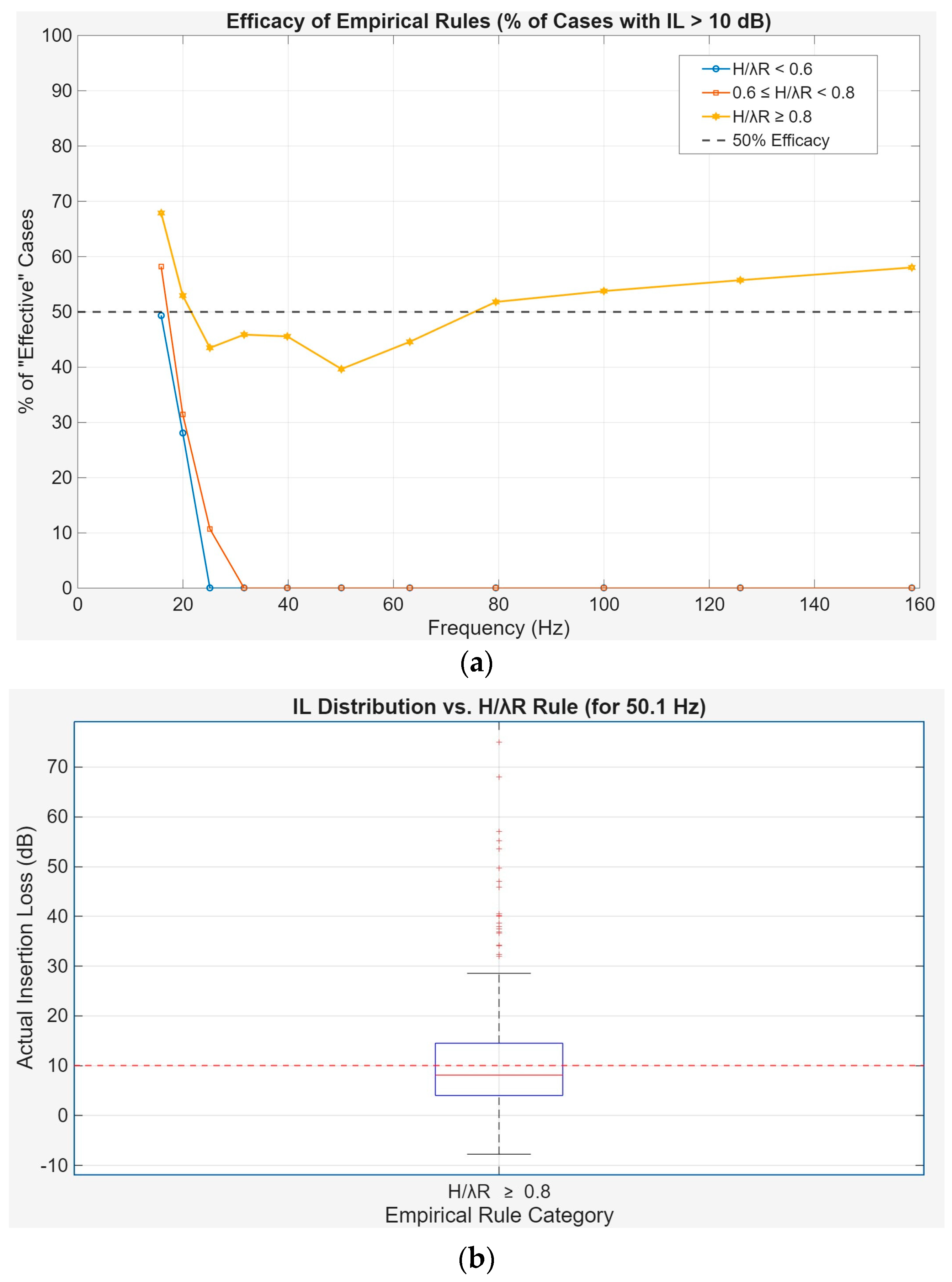
To benchmark the performance of the developed machine learning models, the predictive accuracy of a common empirical guideline for trench barrier design was first assessed. This rule of thumb correlates isolation effectiveness with the ratio of trench depth (H) to the Rayleigh wavelength (λR), suggesting a threshold of H/λR > 0.6 for effective performance. The extensive FEM dataset is therefore used to validate the reliability of this established principle across a wide frequency range. Figure 6 presents a statistical analysis of the relationship between the H/λR ratio and the simulated Insertion Loss (IL). Figure 6a expands this analysis across the entire frequency spectrum, plotting the percentage of ‘effective’ cases (IL > 10 dB) for each rule category. Figure 6b provides a detailed distributional analysis for a representative frequency of 50.1 Hz, focusing on the cases considered ‘very effective’ by the empirical rule (H/λR ≥ 0.8).

Figure 6a confirms that the H/λR < 0.6 category consistently fails to provide reliable isolation. More importantly, even for the H/λR ≥ 0.8 category, the probability of achieving an effective IL is highly frequency-dependent and often falls short of the reliability required for engineering design, hovering around a 50–60% success rate in the critical 40–60 Hz range. Figure 6b shows a wide spread of outcomes for the category (H/λR ≥ 0.8). For a representative frequency of 50.1 Hz, we observe a substantial range of performance. The median IL of approximately 8 dB falls short of the 10 dB efficacy threshold—a common benchmark representing a meaningful (90%) energy reduction. In practical terms, this means that despite adhering to the guideline, more than half of the scenarios failed to deliver a truly significant level of attenuation. This unreliability is not an isolated issue, as Figure 6a confirms that the rule’s performance varies unpredictably across the frequency spectrum. This discrepancy between the empirical rule’s predictions and the complex outcomes observed in the simulations provides the central motivation for this study. It highlights the necessity of more sophisticated, data-driven models capable of capturing the intricate interactions between soil and geometric parameters.

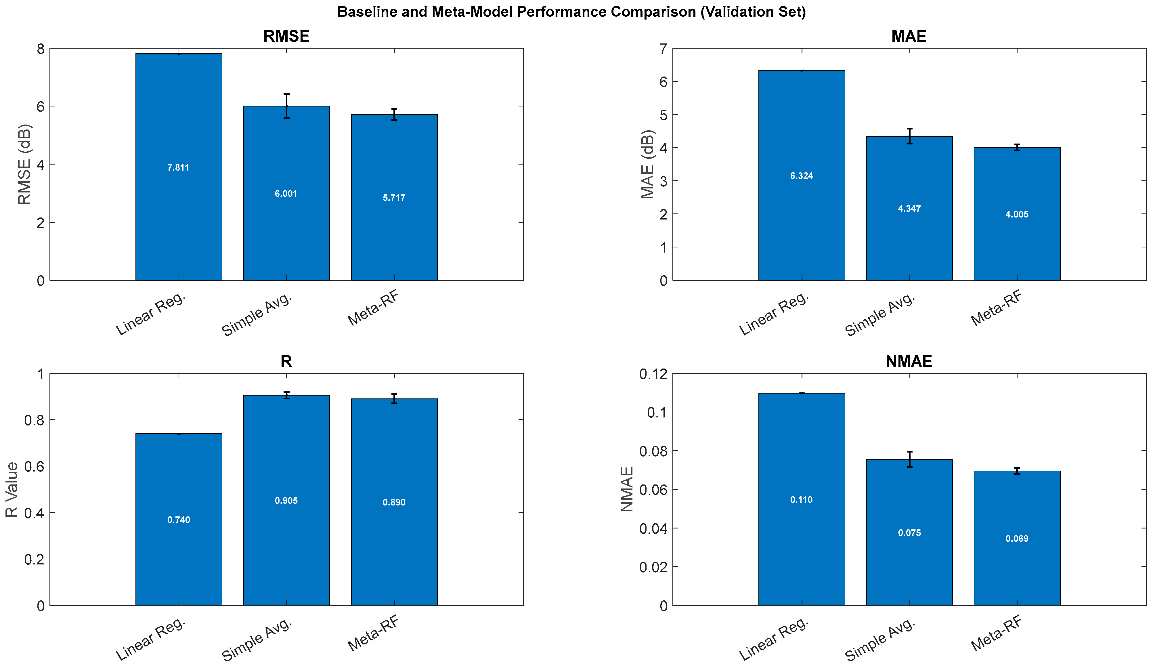
To rigorously evaluate the benefit of the proposed meta-model, a comparative analysis was conducted against simpler baseline methods. Figure 7 presents the performance metrics of the Meta-RF model alongside two such baselines: a Multiple Linear Regression model and a Simple Average ensemble. This comparison serves to quantify the value added by increasing model complexity, from a purely linear approach to a more sophisticated stacking ensemble. The models presented in the comparison are: (i) Multiple Linear Regression, which models a direct linear relationship between the ten primary input features (geometric and material properties) and the resulting Insertion Loss (IL); (ii) Simple Average Ensemble, a straightforward ensemble approach where the final prediction is the arithmetic mean of the outputs from the three individual base models (ANN, SVM, and RF), and (iii) Meta-RF, a Random Forest meta-learner trained on an enriched feature set composed of the predictions from the three base models in addition to the ten original primary input features.

The results shown in Figure 7 clearly indicate that the Multiple Linear Regression model is insufficient for this task, exhibiting high prediction errors (e.g., RMSE ≈ 7.81) and a low correlation (R ≈ 0.74), which confirms the highly non-linear nature of the problem. A substantial improvement is achieved by the Simple Average ensemble, which dramatically reduces errors (RMSE ≈ 6.00) and increases correlation (R ≈ 0.90), demonstrating the inherent value of combining the diverse base models. The more sophisticated Meta-RF model provides a further, gain in performance by achieving the lowest absolute errors (RMSE ≈ 5.72 and MAE ≈ 4.01). Having demonstrated its superiority over simpler baselines, the Meta-RF model’s performance is, in the following sections, compared against the individual models.

4.2. Overlapping of Predicted Values vs. Numerical Values

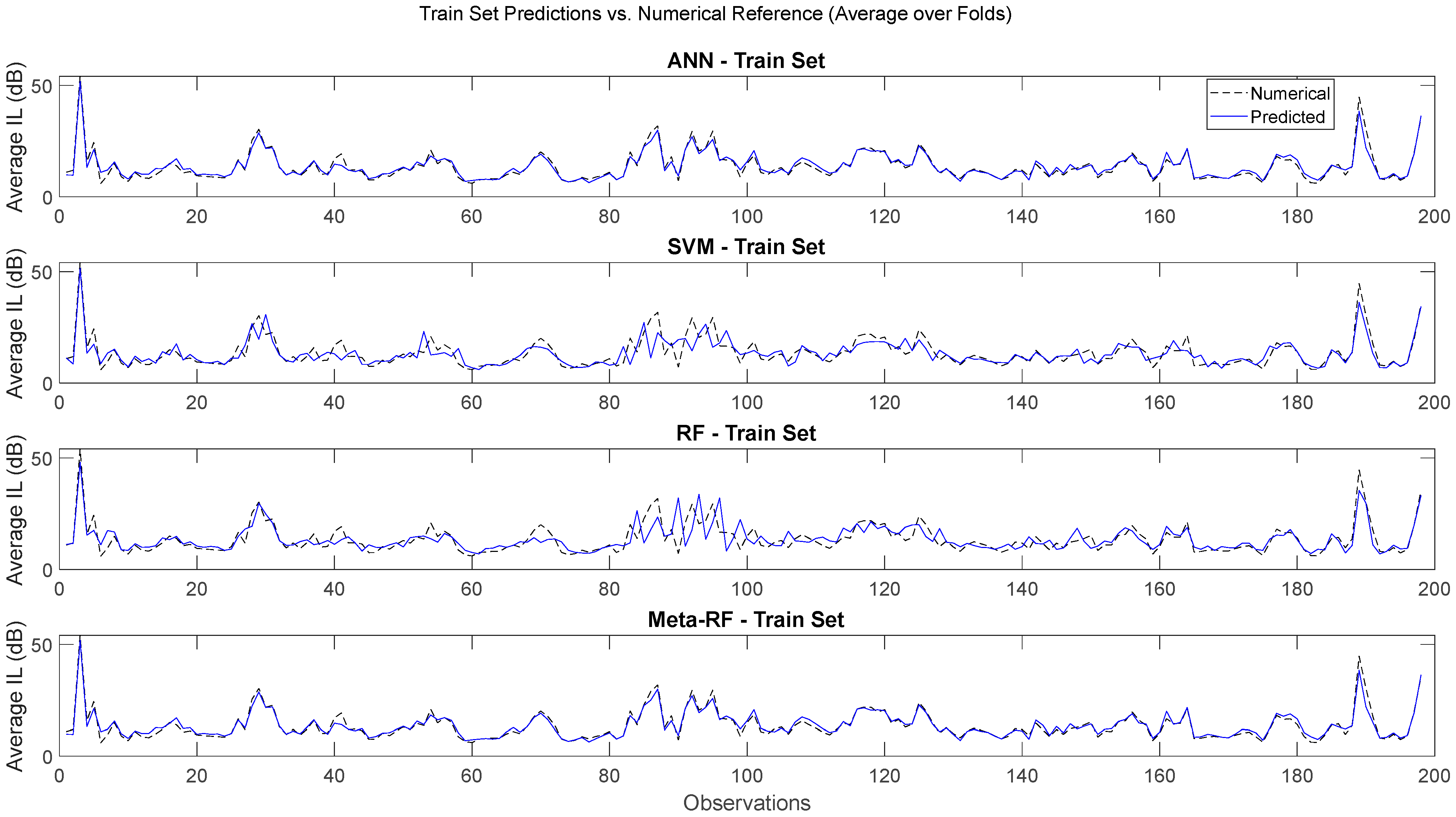
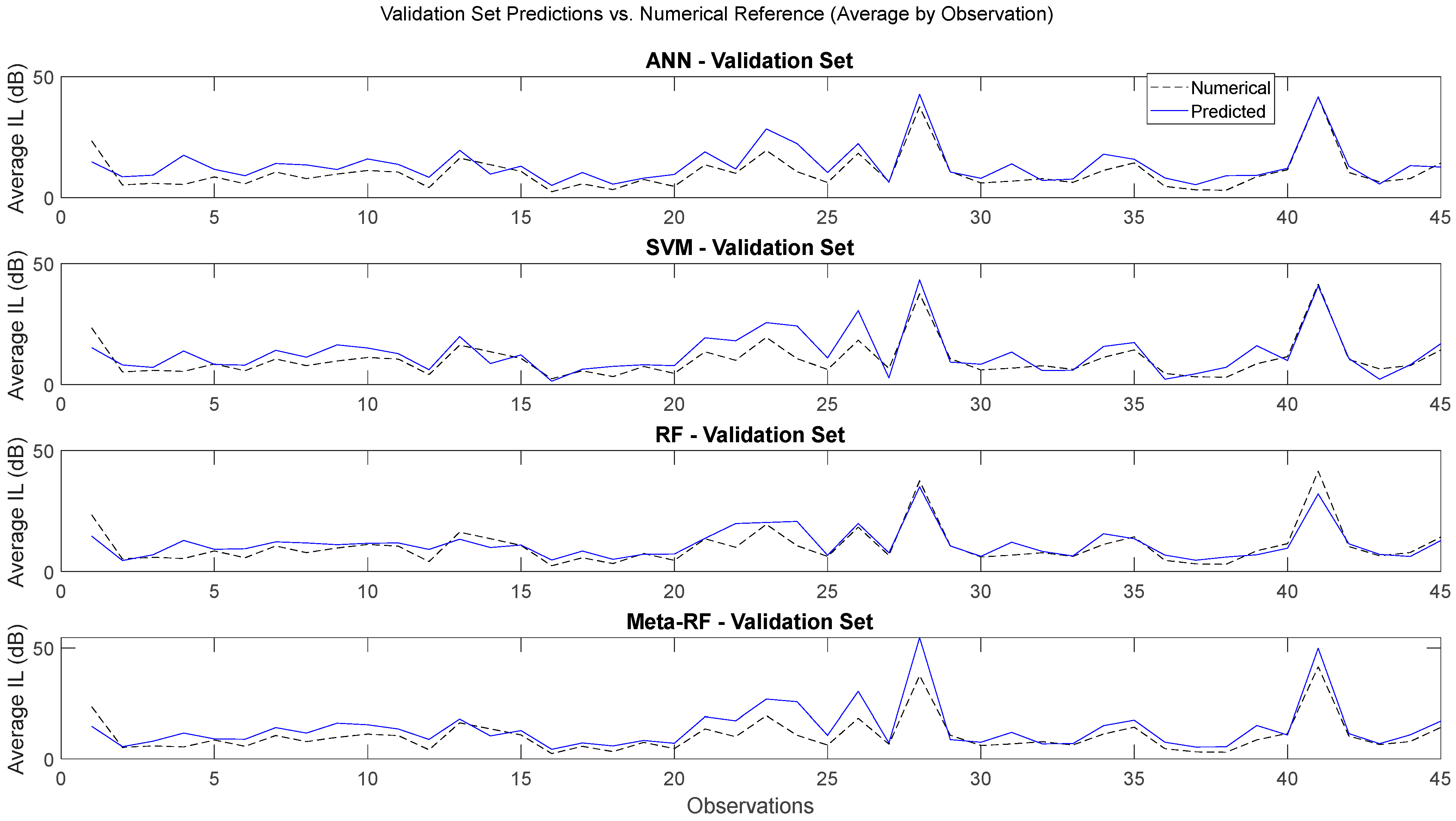
Figure 8 and Figure 9 present a visual comparison between each model predicted values and the numerical reference, for the training set and validation set, respectively.

Figure 8 demonstrates the predictive performance of the Artificial Neural Network (ANN), Support Vector Machine (SVM), Random Forest (RF), and Meta-RF models on their training datasets, comparing their average predictions against the numerical reference values.

All models exhibit a strong agreement between the numerical and predicted curves, indicating that they were able to effectively learn the underlying patterns of the training data. The general shape of the IL response, including its fluctuations and peaks, is accurately reproduced, demonstrating that the models successfully captured the complex relationships among the input variables.

The ANN model shows an excellent fit, with the predicted curve nearly overlapping the reference across most of the observation range. This suggests a high modeling capacity and strong ability to capture nonlinearity in the data. However, in some regions, the predictions appear slightly smoother than the numerical reference, which may reflect a mild regularization effect or a limited network complexity preventing overfitting.

The SVM model also demonstrates a good overall agreement, though minor discrepancies are noticeable near the IL peaks, particularly between observations 60 and 120. Despite these local deviations, the model maintains a consistent and stable performance over the entire dataset.

The Random Forest captures the main trends of the reference curve, though it exhibits higher local variability and small oscillations, especially in the mid-observation range (approximately 70–110). This behavior is consistent with the inherent discrete nature of tree-based models, where the averaging of multiple decision trees can introduce slight irregularities. Nevertheless, the overall fit remains satisfactory and the model clearly reproduces the dominant trends of the numerical data.

The Meta-RF ensemble achieves the closest overall match to the numerical reference. The predicted curve appears smoother and more stable than that of the RF, while maintaining the fidelity of the ANN and SVM predictions. This indicates that the ensemble effectively integrates the strengths of the individual models, reducing their specific biases and enhancing overall accuracy. The Meta-RF therefore provides a robust and well-balanced representation of the training data.

Figure 9 illustrates the predictive performance of the Artificial Neural Network (ANN), Support Vector Machine (SVM), Random Forest (RF), and Meta-RF models on the validation dataset, comparing their average predicted values against the numerical reference. The curves represent the mean response across validation folds, providing an overview of each model’s generalization ability to unseen data.

All models exhibit a reasonable agreement between the predicted and numerical curves, although the alignment is less pronounced than in the training phase. This reduction in correspondence is expected, since the validation dataset consists of unseen observations and therefore represents a more rigorous assessment of the models’ predictive robustness. Nevertheless, the main trends and overall shape of the IL response are satisfactorily reproduced, indicating that the models retained the capacity to capture the essential relationships learned during training.

The ANN model maintains a generally coherent fit, with the predicted curve closely following the numerical reference throughout most of the observation range. Minor deviations are visible near the IL peaks, suggesting a slight degradation in precision when generalizing beyond the training data. This reflects the model’s strong non-linear learning ability but also indicates some sensitivity to data variability in unseen conditions.

The SVM model displays smooth and stable predictions that adequately track the overall reference pattern, though it tends to underestimate higher IL values, particularly around pronounced peaks. Such underestimation is consistent with the model’s regularization characteristics, which limit overfitting at the expense of responsiveness to local maxima.

The RF model captures the dominant fluctuations of the numerical reference, yet presents small oscillations and localized deviations, a behavior typical of tree-based ensembles due to their discrete partitioning of the input space. Despite this, the RF achieves a solid overall performance, preserving the global dynamics of the IL distribution.

The Meta-RF ensemble ends up providing the closest overall agreement with the numerical reference among all tested models, but with a very small difference to the RF model. The predicted curve exhibits slightly enhanced smoothness and stability relative to the RF, while maintaining the non-linear adaptability of the ANN and the regularization benefits of the SVM. This confirms that the ensemble successfully integrates the complementary strengths of the base learners, reducing their individual biases and improving predictive accuracy.

In summary, all models demonstrate adequate generalization to unseen data. Although the Meta-RF model provides the most balanced and reliable predictions—highlighting the advantage of ensemble learning for modeling complex and non-linear relationships in validation scenarios—the improvement over the RF model remains marginal.

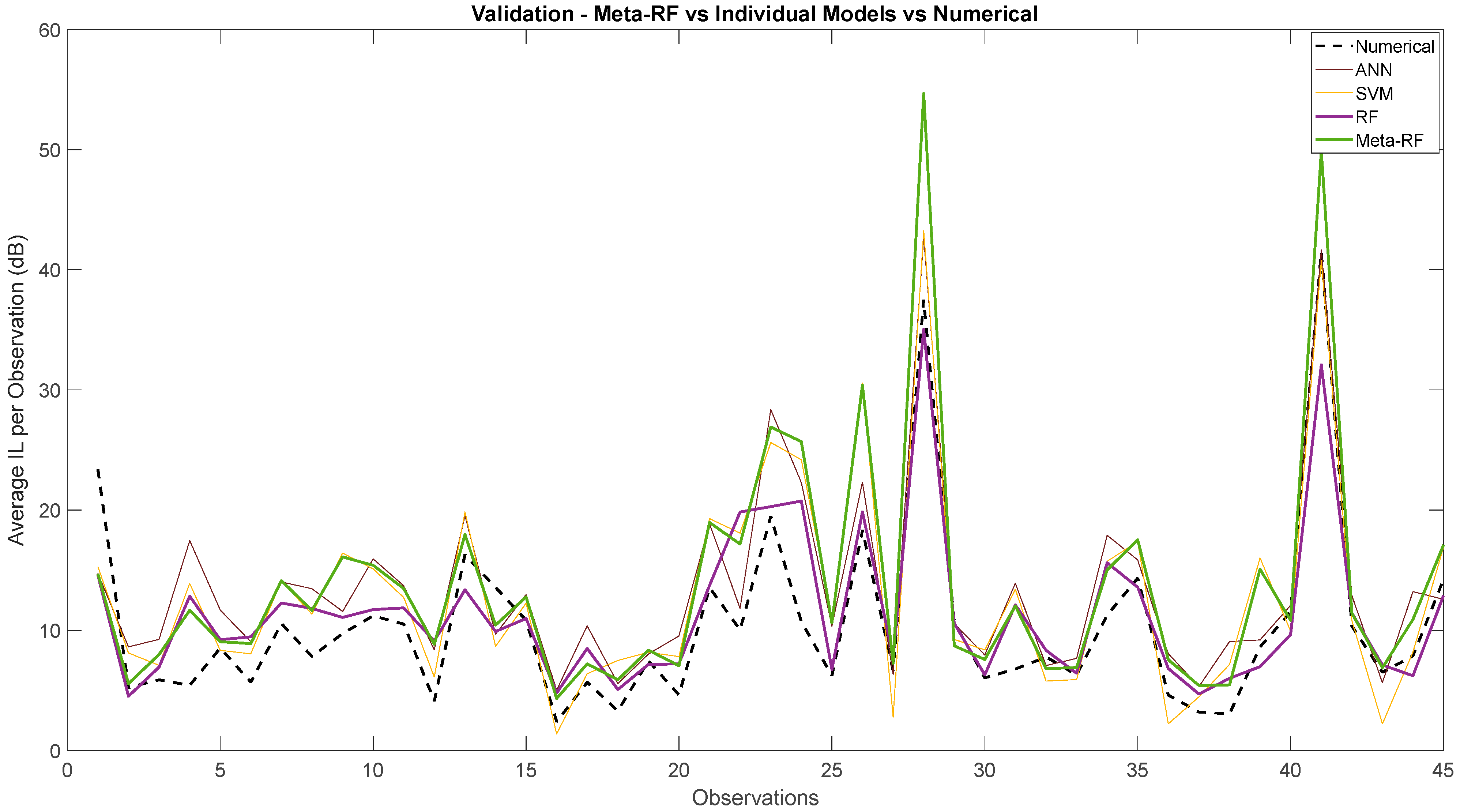
Figure 10 presents a global visualization of the Validation Set predictions, comparing the Artificial Neural Network (ANN), Support Vector Machine (SVM), Random Forest (RF), and Meta-Random Forest (Meta-RF) models against the numerical reference. While all four models demonstrate a capacity to follow the general trends of the IL values, this closer inspection reveals complex behaviors and significant differences in their predictive accuracy, especially at the high-amplitude peaks.

The Meta-RF model is highly reactive to the data’s fluctuations. However, it exhibits a clear tendency to significantly overestimate the magnitude of the most critical peaks. This is starkly visible at observation 28, where the numerical peak is around 37 dB, but the Meta-RF prediction wildly overshoots to approximately 55 dB. A similar, though less extreme, overestimation occurs at the peak near observation 41, where the Meta-RF reaches ~48 dB against a numerical value of ~42 dB. This behavior suggests that while the meta-model is sensitive, it can be unstable and unreliable at predicting extreme events.

In direct contrast, the individual RF model shows a consistent tendency to underestimate the highest peaks. At observation 28, its prediction (~34 dB) is closer to the numerical value than the Meta-RF model, but still an underestimation. At observation 41, this undershoot is even more pronounced, with a prediction of only ~33 dB against the numerical peak of ~42 dB. The RF provides a more conservative and stable, but less accurate, prediction at these high amplitudes.

The ANN and SVM models produce generally smoother predictions. They also significantly underestimate the most prominent peak at observation 28, performing similarly or slightly worse than the individual RF in that instance. However, at other peaks, such as near observation 41, they track the numerical value more closely than the RF, though not as well as the Meta-RF tracks the general trend.

In summary, this comparative analysis reveals a complex trade-off with no single model being universally superior on this validation set. The Meta-RF, while capturing some dynamics well, suffers from severe overestimation at critical peaks, making it unreliable. The individual RF provides a more stable but consistently conservative (underestimated) prediction. The ANN and SVM offer smoother, more generalized predictions but also lack precision at the most important high-amplitude events.

4.3. Sensitivity Analysis of the Input Parameters

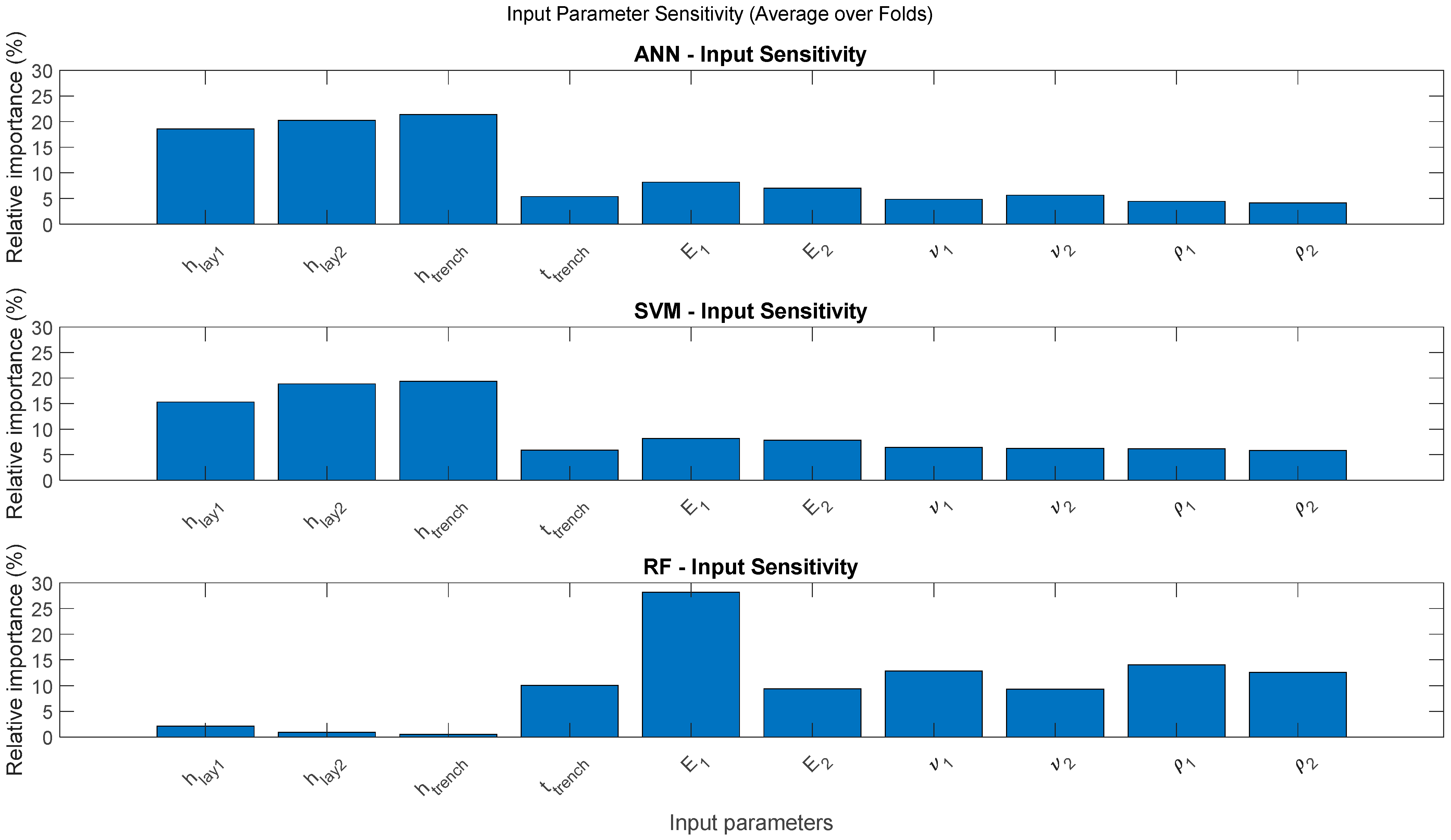
Figure 11 offers a comparative analysis of the input parameter sensitivity for the Artificial Neural Network (ANN), Support Vector Machine (SVM), and Random Forest (RF) models. This visualization, displaying the relative importance of each input parameter (averaged over cross-validation folds) for each model, provides important insights into how these distinct ML algorithms prioritize information when predicting Insertion Loss (IL).

Table 3. Input parameters.

Symbol	Meaning
hlay1	Thickness of the first layer.
hlay2	Thickness of the second layer.
htrench	Trench height.
ttrench	Trench thickness.
E1, E2	Young’s modulus (layers 1 and 2).
v1, v2	Poisson’s ratio (layers 1 and 2).
${\rho }_1$$,\rho$2	Material density (layers 1 and 2).

presents the meaning of all the input parameters of Figure 9.

A comparison of the input parameter importance across the models reveals significant divergences in their learned feature hierarchies. While some similarities exist between the ANN and SVM, the RF model adopts a fundamentally different approach to solving the problem.

For the ANN model, it is immediately visible that the main geometric dimensions are the most influential input parameters. Specifically, the trench depth (h_trench), and the layer thicknesses (h_lay1 and h_lay2) are the three most dominant features, each with a relative importance of approximately 15–20%. This suggests that the ANN heavily relies on these physical dimensions as primary drivers for its IL predictions. Following these, the material properties of the layers, particularly the Young’s modulus (E₁ and E₂), exhibit moderate importance, while the remaining parameters, including trench thickness (t_trench), show a comparatively minor impact.

The SVM model’s sensitivity analysis presents a remarkably similar hierarchy to the ANN, again underscoring the dominance of geometric parameters. The same three features—h_trench, h_lay2, and h_lay1—are clearly the most influential, collectively accounting for over half of the model’s predictive logic. As with the ANN, the Young’s modulus (E₁, E₂) are of secondary importance, and all other material properties have a limited influence. This strong alignment suggests that both the ANN and SVM learned to prioritize a similar, geometry-focused interpretation of the problem.

The RF model exhibits a fundamentally distinct and contrasting understanding of input parameter importance. In a major divergence from the other two models, it identifies the Young’s Modulus of the first layer (E₁) as the single most influential parameter, with a relative importance approaching 28%. The RF model distributes the remaining importance across other material properties, with the properties of the first layer (ν₁, $\rho$₁) and the trench thickness (t_trench) also showing significant influence. Most strikingly, the large-scale geometric parameters that were paramount for the ANN and SVM—h_lay1, h_lay2, and h_trench—demonstrate remarkably low, near-zero importance for the RF model.

This input sensitivity analysis reveals that while all three models are capable of successfully predicting IL values, they achieve this by learning and emphasizing different sets of input features. The ANN and SVM models primarily rely on the large-scale geometric dimensions as their core drivers, aligning with a more intuitive physical interpretation of how structural changes affect wave propagation. In contrast, the RF model diverges significantly, instead prioritizing the stiffness of the first layer (E₁) and other material properties. The minimal importance assigned by the RF model to the primary layer and trench depths highlights that it extracts predictive patterns from a fundamentally different and less intuitive feature hierarchy.

4.4. Evaluation Metrics—RMSE, MAE, NMAE, and R

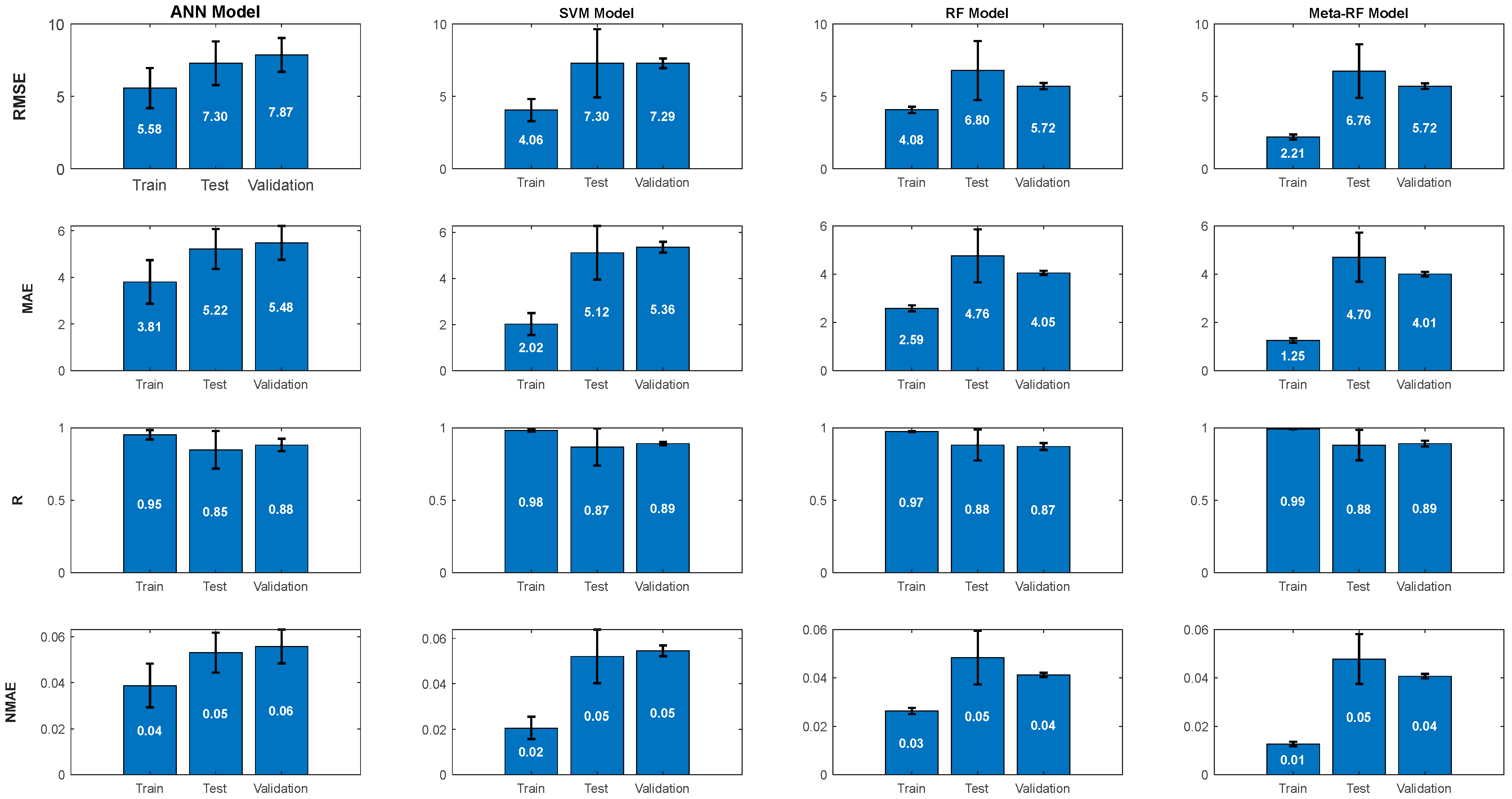
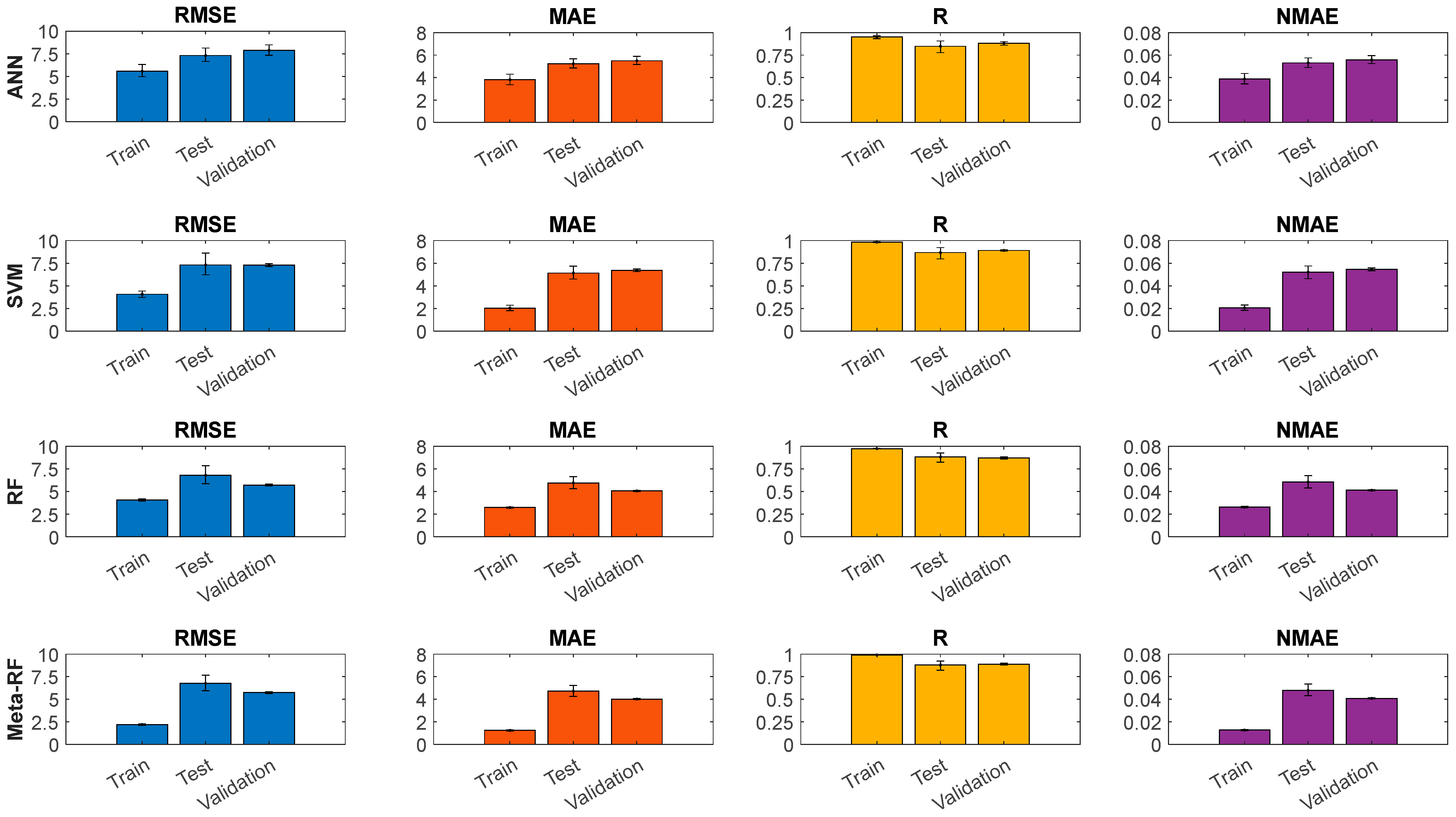
Figure 12 presents the evaluation metrics obtained from the ANN, SVM, RF, and Meta-RF models. For each model, Root Mean Squared Error (RMSE), Mean Absolute Error (MAE), Correlation Coefficient (R), and the Normalized Mean Absolute Error (NMAE), are presented across the training, test, and validation datasets, including uncertainty estimates (error bars).

For all four models, the performance evaluation metrics RMSE, MAE, and NMAE generally increase from the training set to the test and validation sets, while the correlation coefficient (R) decreases. This behavior is typical of ML models, reflecting an expected and slight reduction in predictive accuracy when generalizing to unseen data.

On the training set, all models exhibit a strong ability to learn the data, but the Meta-RF model demonstrates a superior fit, achieving the lowest errors by a clear margin (RMSE = 2.21 dB, MAE = 1.25, and NMAE = 0.01) and the highest correlation (R = 0.99). The SVM and RF models show the next-best performance, with very similar and highly competitive results (e.g., RMSE of 4.06 dB and 4.08 dB, respectively). The ANN model also shows a strong training fit (RMSE = 5.58 dB), though it is the least precise of the four on the training data. This indicates that all models are capable of learning the underlying non-linear relationships, with the ensemble methods showing a distinct advantage in fitting accuracy.

On the unseen test set, the Meta-RF and RF models are the clear top performers, achieving the lowest absolute errors with RMSE values of 6.76 dB and 6.80 dB, respectively. The ANN and SVM models are less accurate on this set, with higher and nearly identical RMSE values of approximately 7.30 dB. All models maintain a strong correlation coefficient, with the RF, Meta-RF, and SVM all achieving R = 0.87–0.88.

For the final validation set, the trend is confirmed: the Meta-RF and RF models are again superior, achieving the joint-lowest RMSE of 5.72 dB and the lowest MAE values (4.01 and 4.05, respectively). The SVM (RMSE = 7.29 dB) and ANN (RMSE = 7.67 dB) perform less accurately in terms of absolute error. In terms of correlation, the Meta-RF and SVM achieve the highest R value (0.89), closely followed by the ANN and RF (0.88 and 0.87).

In conclusion, this analysis reveals a clear performance hierarchy. While all models demonstrate strong learning capabilities, the RF-based methods consistently outperform the ANN and SVM on unseen data. The individual RF model proves to be the best-performing of the base learners. Crucially, the Meta-RF ensemble emerges (marginally) as the best model overall, as it not only achieves the tightest fit on the training data but also delivers the best (or joint-best) performance on the validation set across all key metrics, providing the lowest absolute errors with a very high correlation coefficient. This underscores that the stacking ensemble strategy in achieving accurate and reliable predictions has a slim edge over the RF model.

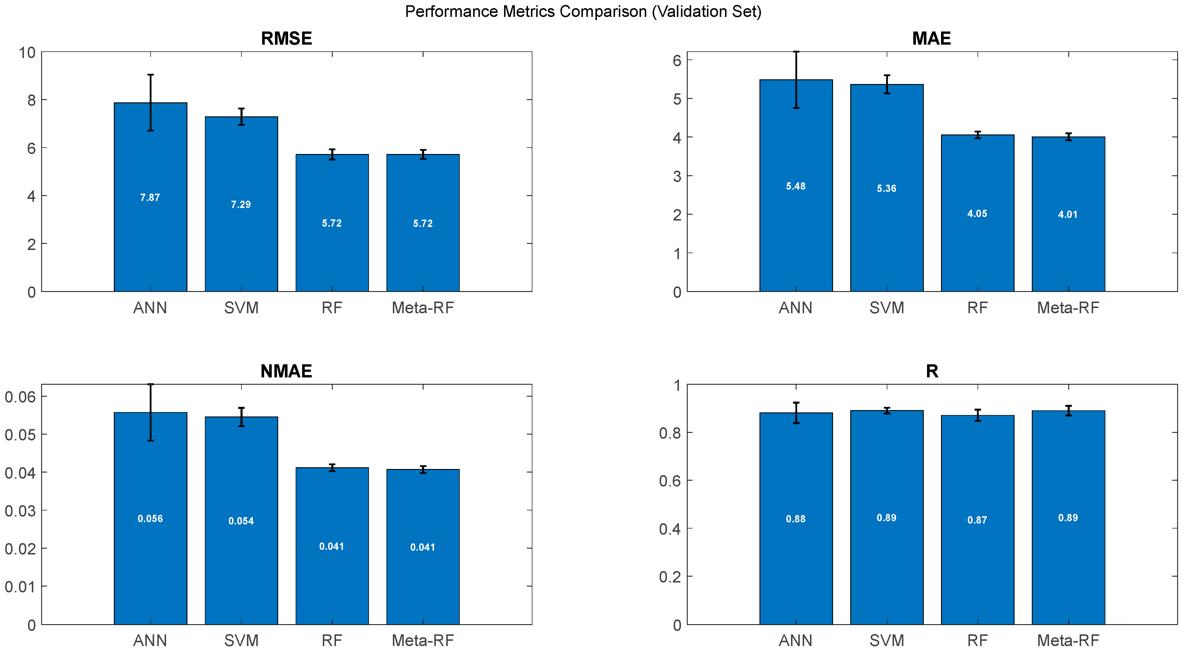
Figure 13 presents a comparative summary of the models’ performance on the validation set, confirming the trends observed in the test set and highlighting a clear performance hierarchy.

Analyzing Figure 13, we can observe that the RF and Meta-RF models are demonstrably superior in minimizing absolute prediction errors, achieving the lowest and identical RMSE (5.72 dB) and the lowest MAE (≈4.01–4.05 dB) values. The ANN and SVM models perform less accurately, exhibiting significantly higher absolute errors (RMSE > 7.29 dB).

An interesting trade-off is observed in the correlation coefficient (R), where the SVM and Meta-RF (R = 0.89) slightly outperform the individual RF (R = 0.87).

In conclusion, this analysis confirms that while all models generalize effectively, the Meta-RF model emerges as the most robust and well-balanced performer, although with a very narrow advantage over the RF model. It consistently achieves the lowest absolute prediction errors (RMSE, MAE, NMAE) while maintaining a high correlation coefficient, thereby validating the effectiveness of the advanced stacking ensemble approach for this problem.

Addressing the trade-off in the performance characteristics of the models, it is visible that the Random Forest (RF) model consistently achieves one of the lowest absolute errors (RMSE and MAE), indicating a high degree of point-by-point accuracy. However, it simultaneously displays a comparatively lower correlation coefficient (R) than both the ANN and SVM models.

This can be attributed to the fundamental architectural differences in the algorithms. The RF, as an ensemble of decision trees, excels at capturing complex, non-linear relationships with high local accuracy. Its structure is highly effective at minimizing individual prediction errors across the dataset. In contrast, the ANN (with logsig activation functions) and the SVM (with a Gaussian kernel) are models that generate inherently smoother functional forms. This intrinsic smoothness may allow them to better capture the global trend and overall shape of the data across all observations, leading to a higher correlation coefficient, even if their point-by-point error is marginally higher than that of the RF. Therefore, this trade-off can be a reflection of the models’ different strategies: the RF prioritizes local predictive precision, while the ANN and SVM are better suited to capturing the global data trend in this specific evaluation context.

4.5. Statistical Analysis of the ML Models

Figure 14 shows the Shapiro–Wilk normality test results for all models and datasets. The figure displays the negative logarithm (−log10) of the p-values from the Shapiro–Wilk normality test for RMSE, MAE, R, and NMAE across the train, test, and validation sets for all models (ANN, SVM, RF, Meta-RF). The red dashed line indicates the significance level of p = 0.05, corresponding to −log10(0.05) ≈ 1.3. Values above this line signify the rejection of the null hypothesis of normality.

For the vast majority of metrics and datasets, across all models, the bars are significantly above the −log10(p-value) = 1.3 threshold (corresponding to a p-value of 0.05), often exceeding 15 or even 20. This indicates that the distributions of the performance metric values (RMSE, MAE, R, NMAE) obtained from each fold of the cross-validation are not normally distributed for any of the models (ANN, SVM, RF, Meta-RF) across the training, test, and validation sets. This non-normality is a common characteristic in complex ML model evaluations and justifies the utilization of robust, non-parametric statistical methods, such as Bootstrap confidence intervals (see Figure 15), which do not rely on assumptions of data normality.

Figure 15 displays the 95% Bootstrap Confidence Intervals (CI) for all the ML models performance metrics: RMSE, MAE, R, and NMAE. The results are presented for all the datasets, with error bars indicating the range of the confidence interval.

During the training phase, the models demonstrated a clear hierarchy in fitting prowess. The Meta-RF model achieved by far the tightest fit, evidenced by its exceptionally low RMSE (≈2.21 dB) and MAE (≈1.25 dB), and a near-perfect R value (≈0.99). The individual RF (RMSE ≈ 4.08 dB) and SVM (RMSE ≈ 4.06 dB) models also exhibited strong learning capabilities, with the ANN model showing a solid but comparatively less precise fit (RMSE ≈ 5.58 dB). This confirms that all models effectively learned the training data, with the ensemble methods showing a distinct advantage.

On the unseen test and validation sets, which assess the models’ generalization capabilities, a consistent performance ranking emerges. The Meta-RF model consistently provides the most accurate predictions, achieving the lowest absolute errors across both sets (e.g., Validation RMSE ≈ 5.72 dB and MAE ≈ 4.01 dB). The individual RF model is the clear second-best performer (almost tied with the Meta-RF model) and the strongest of the base learners (Validation RMSE ≈ 5.72 dB and MAE ≈ 4.05 dB). The SVM and ANN models lag behind, exhibiting significantly higher prediction errors on unseen data (Validation RMSE ≈ 7.29 dB and ≈7.87 dB, respectively).

Regarding the correlation coefficient (R) on the validation set, the Meta-RF and SVM models achieve the highest value (≈0.89), indicating the best ability to capture the overall data trend, closely followed by the ANN and RF models (≈0.88 and ≈0.87, respectively).

These analyses, supported by the Bootstrap confidence intervals (CIs), lead to a clear conclusion. The narrow CIs in the training phase reflect high precision in fitting, while the wider CIs in the test and validation phases underscore the increased uncertainty inherent in predicting unseen data. The overlapping CIs for the RMSE and MAE metrics between the RF and Meta-RF models on the validation set suggest their top-tier performance in error minimization is statistically similar. However, considering all metrics together, the Meta-RF model emerges as the superior and most well-balanced performer, consistently achieving the lowest absolute errors while also maintaining the highest correlation on the critical validation set.

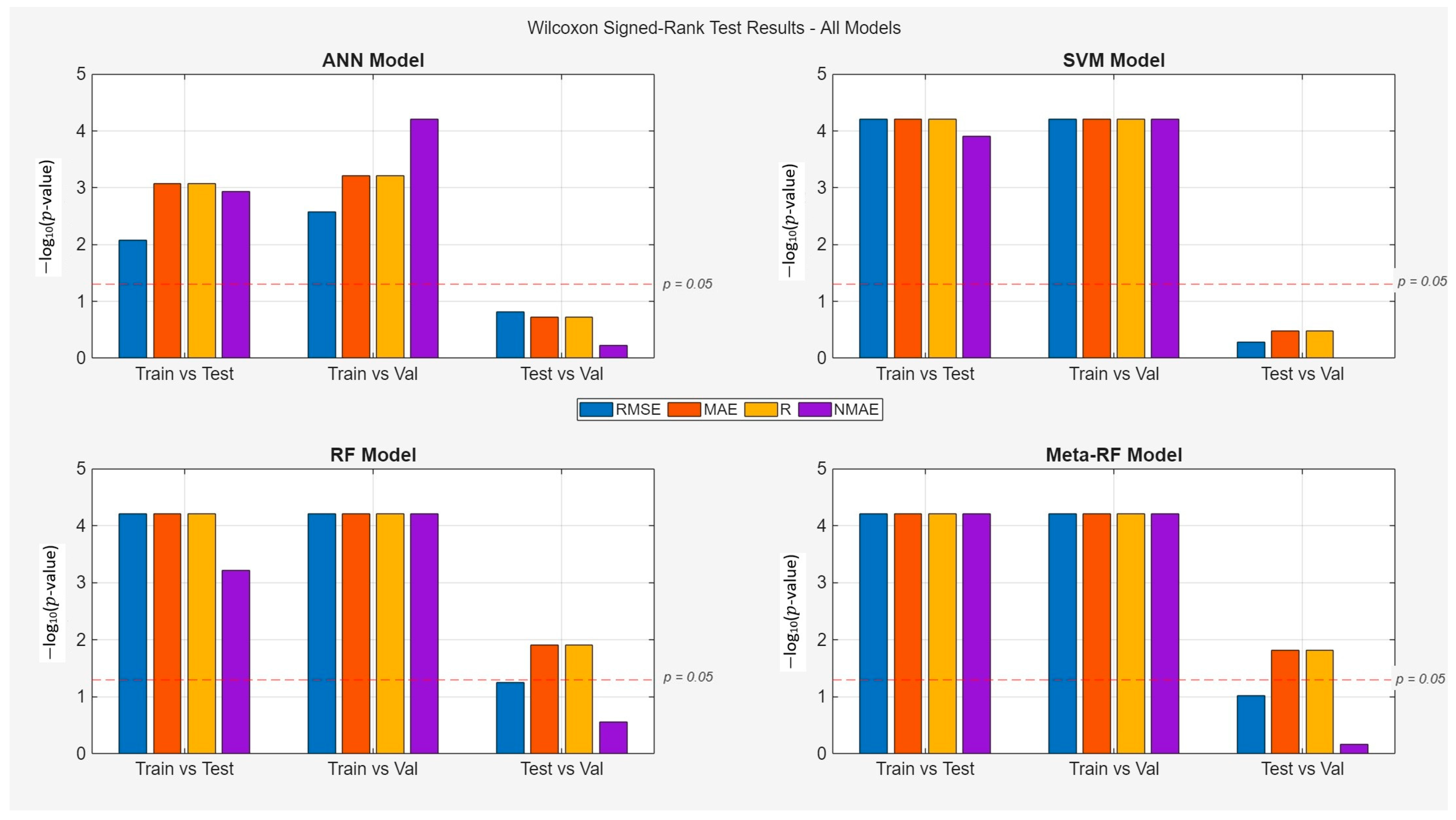
Figure 16 presents the statistical validation of the models’ generalization gap and performance stability. It displays the results of the Wilcoxon Signed-Rank test, used to determine if the performance differences between the training, test, and validation sets are statistically significant.

A rigorous statistical evaluation was performed using the Wilcoxon Signed-Rank test to assess the performance differences between the training, test, and validation sets for all models, with the results presented in Figure 16. This analysis is critical to quantitatively address the generalization gap—the expected performance degradation when a model transitions from seen to unseen data.

The results demonstrate that all four models exhibit a statistically significant generalization gap, which is the expected and correct behavior for properly trained, non-trivial models. For the SVM and Meta-RF models in particular, the −log₁₀(p-value) bars in both the Train vs. Test and Train vs. Val comparisons are consistently and significantly above the p = 0.05 significance threshold. This result is of primary importance as it confirms that the models are non-trivial and that the evaluation is not biased by issues such as data leakage, which would manifest as a lack of a statistically significant difference between training and validation performance.

Furthermore, the Test vs. Val comparison assesses the stability of the models’ generalization performance across two distinct unseen datasets. Here, the results are more varied. The ANN and SVM models show high stability, with no statistically significant differences between their test and validation set metrics. In contrast, the RF model shows statistically significant variability in its MAE and R metrics, while the Meta-RF model exhibits even broader significant differences across MAE, R, and NMAE. This indicates that while all models generalize, the ANN and SVM do so with greater performance consistency when faced with different sets of new data.

In conclusion, the Wilcoxon Signed-Rank test provides two key insights. First and foremost, it validates the integrity of the training and evaluation methodology by confirming a significant generalization gap for all models. Second, it provides a nuanced understanding of model stability, highlighting the different ways each model’s performance varies when encountering new data.

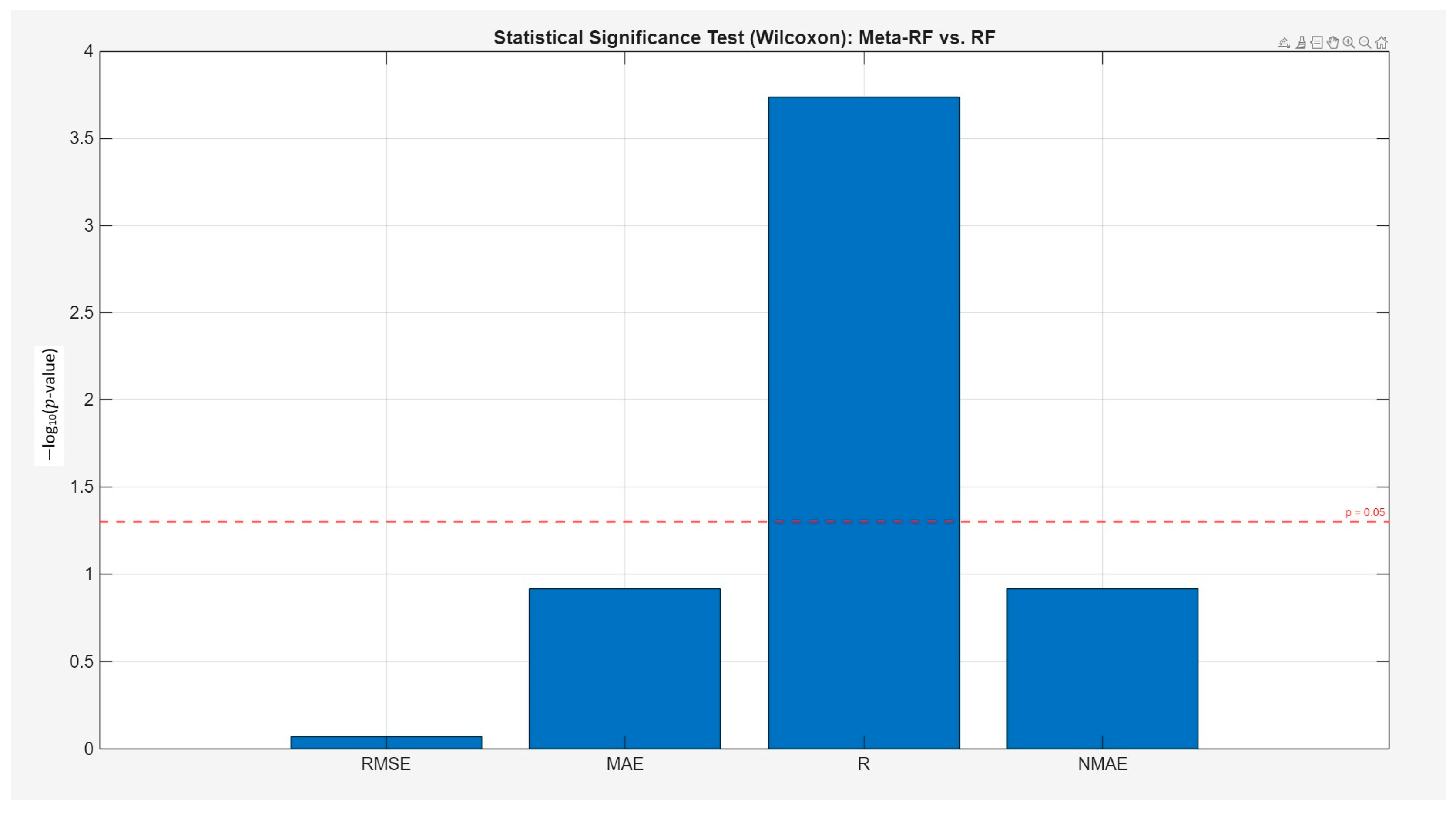
A statistical significance analysis was performed to formally address the question of whether the advanced Meta-RF model provides a meaningful improvement over the best-performing individual model, the RF. A paired Wilcoxon Signed-Rank test was conducted on the performance metrics obtained from the 15 cross-validation folds, with the results presented in Figure 17.

The analysis provides a nuanced conclusion. For the absolute error metrics (RMSE, MAE, and NMAE), the results indicate that there is no statistically significant difference between the Meta-RF and the individual RF model (p > 0.05 for all three). This confirms that the marginal improvements in average error observed previously are not statistically robust.

However, for the correlation coefficient (R), the test reveals a highly statistically significant difference between the two models (p ≈ 0.0002). This demonstrates that while the Meta-RF does not significantly reduce the magnitude of prediction errors compared to the already powerful RF model, its added complexity is justified by a statistically significant and robust improvement in its ability to capture the overall trend and shape of the data. This finding addresses the trade-off between complexity and benefit, showing that the two-stage approach yields a specific, measurable, and statistically valid advantage in predictive quality.

4.6. Results for Specific Scenarios

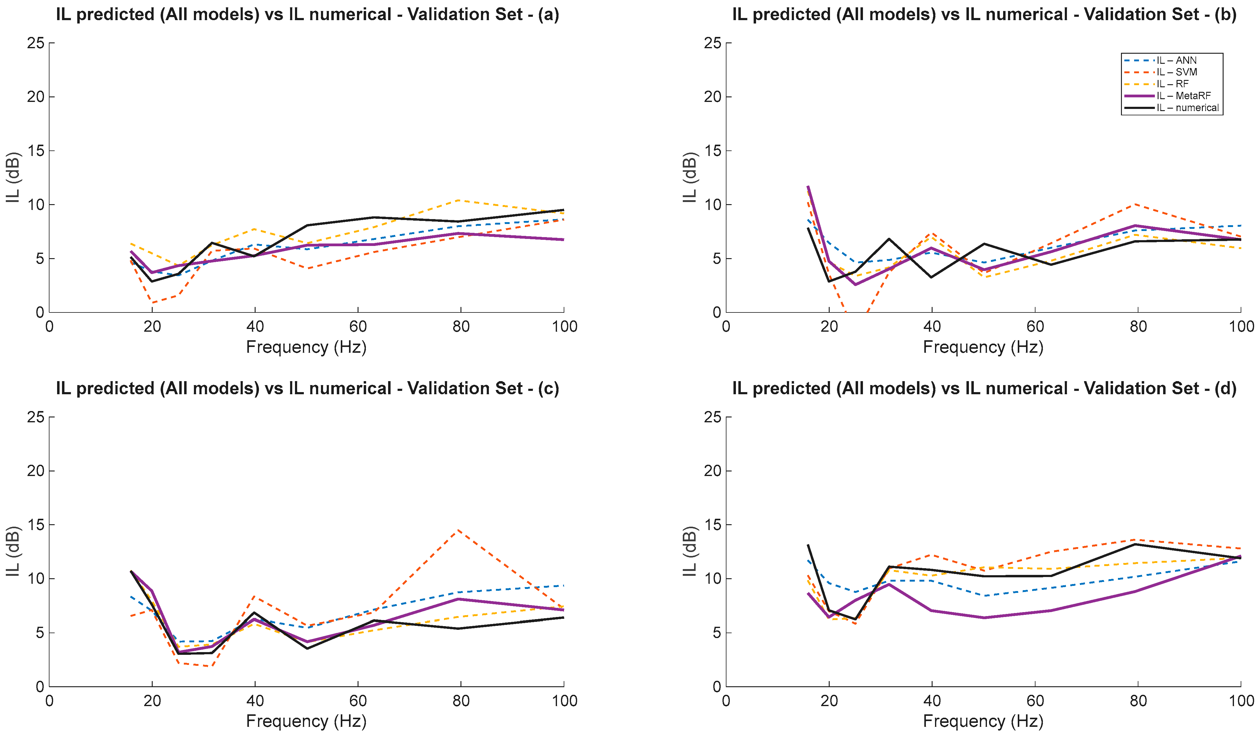
Figure 18 illustrates the Insertion Loss (IL) predictions of the models (ANN, SVM, RF, Meta-RF) compared with numerical results for the validation set across four distinct scenarios (a, b, c, d), plotted as a function of frequency. This comprehensive visualization, informed by the geometric and elastic characteristics in Table 3, allows for an in-depth assessment of model generalization and the underlying physical phenomena.

Table 4. Geometric characteristics and elastic properties of each of the simulations plotted in Figure 18.

Figure 15	Thickness (m)		Trench (m)		Young Modulus (MPa)		Poisson Coefficient		Density (kg/m3)
	Layer 1	Layer 2	Depth	Thickness	Layer 1	Layer 2	Layer 1	Layer 2	Layer 1	Layer 2
(a)	5	5	5	0.23	4.63 × 107	7.36 × 107	0.34	0.36	1677	1958
(b)	4	2	4	0.35	4.30 × 107	6.85 × 107	0.35	0.30	1666	1695
(c)	4	3	4	0.12	6.03 × 107	8.02 × 107	0.32	0.31	1685	1754
(d)	4	2	5	0.14	4.19 × 107	5.81 × 107	0.27	0.32	1610	1818

presents the geometric characteristics and elastic properties of each of the situations shown in Figure 15.

A key observation consistent across all four scenarios is the remarkably high fidelity of the RF and Meta-RF models (dashed yellow line and thick solid purple line, respectively) to the numerical reference (thin solid black line). These models consistently provide the closest match to the numerical IL values, demonstrating its superior robustness and accuracy in generalization across varied physical and geometric conditions. The individual models (ANN, SVM), represented by the blue and red dashed lines, respectively, also track the numerical trends reasonably well, but they exhibit varying degrees of deviation.

For Scenario (a), this configuration is characterized by layers of equal thickness (5 m each), where Layer 2 is stiffer (E = 7.36 × 10⁷ Pa) and denser ($\rho$ = 1958 kg/m³) than Layer 1 (E = 4.63 × 10⁷ Pa, $\rho$ = 1677 kg/m³). The trench depth is 5 m. The numerical IL shows an initial dip at lower frequencies, followed by a general increase towards higher frequencies, resulting in relatively high IL values (ranging from ≈5 dB to ≈10 dB). As frequency increases and wavelengths shorten, the trench’s effectiveness and the resulting IL increase due to a higher Trench Depth/Rayleigh Wavelength (H/λR) ratio. The ANN, RF, and Meta-RF models closely follows this trend with minimal deviation.

Scenario (b) presents a configuration where Layer 1 is thicker (4 m) than Layer 2 (2 m), with a 4 m trench depth. Layer 2 is stiffer but has a very similar density to Layer 1, resulting in a minimal density contrast. The numerical IL values show significant fluctuations, dropping to very low levels (≈3–4 dB) at certain frequencies before rising again. The minimal density contrast likely leads to less significant reflection phenomena at the layer interface, contributing to the overall lower IL values compared to other scenarios.

Scenario (c) shares the same trench depth as scenario (b) (4 m) but features a thicker second layer (3 m vs. 2 m). The numerical IL trend in scenario (c) follows a pattern broadly similar to scenario (b). The RF and Meta-RF models excel at following the numerical curve.

For Scenario (d), this configuration features a significant contrast between the layers, with Layer 2 being considerably stiffer (E = 5.81 × 10⁷ Pa) and denser ($\rho$ = 1818 kg/m³) than Layer 1 (E = 4.19 × 10⁷ Pa, $\rho$ = 1610 kg/m³). The trench depth is 5 m. The numerical IL shows an initial peak around 17 Hz, followed by a significant dip, and then a stable trend with relatively high IL values (ranging from ≈7 dB to ≈12 dB). The combination of the strong physical contrast between layers—which promotes wave reflection and diffraction at the interface—and the relatively deep trench (5 m) likely contributes to the effective overall performance. Furthermore, the softer materials in this scenario compared to others lead to lower wave velocities and shorter wavelengths, resulting in a higher H/λR ratio that enhances the trench’s effectiveness. In this specific scenario, the RF model shows a superior performance, maintaining a very close match to the numerical data.

The analysis confirms that all models perform competently in physically meaningful scenarios. The RF and Meta-RF models, in particular, demonstrate the best overall performances, providing a more robust prediction of IL across the full frequency spectrum, as they likely balance the predictive strengths of the other individual models (ANN and SVM) to account for the complex physical phenomena involved.

4.7. Overall Considerations and Future Perspectives

The use of a high-fidelity FEM simulation framework in this study provided the crucial advantage of generating a comprehensive and clean dataset across a wide parametric space, allowing for the systematic training and evaluation of the machine learning models. We acknowledge, however, the inherent limitations of a purely simulation-based study and the importance of addressing the “sim-to-real” gap, as real-world performance can be influenced by factors not captured in the numerical model, such as soil heterogeneity, material inconsistencies, and ambient measurement noise.

Additionally, while the uniform random sampling employed was sufficient for broad parameter space exploration in this proof-of-concept, future work could benefit from more advanced sampling techniques, such as Latin Hypercube Sampling, to ensure even more efficient coverage.

Nevertheless, it is unquestionable that the application of machine learning methodologies offers a very significant improvement in computational efficiency, particularly for design exploration and parametric studies. While the development of these models requires a significant upfront computational investment, this cost is amortized over their subsequent application.

Table 5. Computational costs of the FEM simulation and Machine Learning model phases.

Phase	Task/Model	Computational Time (Approx.)	Notes
Data Generation	FEM Simulation Database	≈60 h	For all 2000 simulations
Machine Learning	Training Phase		One-time investment
	ANN	≈17 h
	SVM	≈1.3 h	(1 h, 20 min)
	RF	≈4.5 h	(4 h, 30 min)
	Meta-RF	≈4.5 h	(4 h, 30 min)
	Inference Phase	<0.1 s	Per prediction for a full IL curve

provides a comprehensive summary of the computational costs associated with both the initial data generation and the ML model training phases.

The generation of the database, consisting of 2000 individual FEM simulations, required approximately 60 h of processing time on the specified hardware (Intel Core i7-8700 CPU @ 3.20 GHz). Following this, the one-time training of the individual ML models varied in duration, from approximately 1.3 h for the SVM to 17 h for the ANN, with the RF model taking 4.5 h. The subsequent training of the Meta-RF was similar, also around 4.5 h. The crucial benefit, however, lies in the inference time: once trained, any of these ML models can produce a new prediction for a full IL curve in a fraction of a second. This represents a dramatic acceleration compared to the time required for a single FEM run, enabling large-scale analyses that would be computationally prohibitive otherwise.

Future research will therefore focus on validating and refining the developed models with experimental data, which introduces its own set of challenges. Bridging this gap often requires advanced data-driven techniques, not just for prediction, but for signal interpretation itself. For instance, in the field of structural health monitoring, machine learning architectures are effectively used to analyze complex vibration signals from instrumented structures, automatically extracting damage-sensitive features from noisy experimental data [58]. In geotechnical and seismic applications, data-driven methods are essential for classifying and de-noising complex in situ signals to extract meaningful parameters, as demonstrated by Kim et al. [58] in the classification of microseismic data. These studies highlight a powerful synergy: while our work uses ML as a surrogate for a physics-based model, these same techniques will be indispensable for processing and interpreting the complex signatures of physical experiments, a necessary step for future model validation.

Beyond experimental validation, a further step towards building trust in the models involves inspecting their “black-box” nature. Beyond the initial insights from the sensitivity analysis, an important future direction is to enhance the model’s physical interpretability. This could be achieved by integrating state-of-the-art explainable AI (XAI) techniques, such as SHAP (SHapley Additive exPlanations). Employing these methods would offer a granular audit of the trained models, providing a means to verify that their predictive logic aligns with physically sound principles—such as the expected influence of trench geometry and soil property contrasts—instead of relying on spurious statistical correlations. Such an approach aims to move beyond prediction accuracy alone, building models with genuine physical intelligence and thereby increasing their trustworthiness for adoption in engineering practice [59,60].

5. Conclusions

This study investigated the effectiveness of several machine learning models—Artificial Neural Network (ANN), Support Vector Machine (SVM), Random Forest (RF), and a stacked ensemble (Meta-RF)—as computationally efficient surrogates for predicting the Insertion Loss (IL) of open trench barriers for vibration mitigation. The investigation began by confirming the limitations of traditional empirical guidelines, such as the H/λR ratio, which proved to be unreliable predictors due to the complex interplay between the system’s geometric and material properties, thus establishing the need for more sophisticated, data-driven approaches.

The comparative analysis of the individual machine learning models revealed a clear performance hierarchy on unseen data. While the ANN and SVM models demonstrated competent generalization capabilities, the individual Random Forest (RF) model emerged as unequivocally superior, achieving significantly lower prediction errors (e.g., a validation set RMSE of 5.72 dB) and a strong correlation coefficient. This highlights its exceptional ability to capture the complex, non-linear relationships inherent in the wave propagation problem.

The advanced stacking ensemble, the Meta-RF model, was developed to ascertain if combining the predictions of the individual learners could yield further performance gains. The results indicate that the Meta-RF achieved the highest predictive accuracy across most metrics, but by a very marginal amount compared to the individual RF model. For instance, both models registered an identical RMSE of 5.72 dB on the validation set, with the Meta-RF showing a slight advantage in MAE (4.01 vs. 4.05 dB). Crucially, a Wilcoxon Signed-Rank test was performed to assess the statistical significance of the performance difference between the RF and Meta-RF. The results showed no statistically significant difference between the two models for the primary error metrics, confirming that the observed improvement of the Meta-RF is not statistically robust.

This finding has significant practical implications. While the training of the Meta-RF itself was computationally efficient (≈4.5 h), its development is contingent upon the prior training of all three base models, which collectively required over 22 h (ANN: 17 h, RF: 4.5 h, SVM: 1.3 h). Given the minimal and statistically insignificant performance gain, it is reasonable to conclude that the additional complexity and substantial time investment required to build the stacking ensemble may not be justified for many practical engineering applications. The individual RF model, on its own, provides an outstanding balance of high accuracy and more straightforward implementation.

Nevertheless, all the developed ML models proved to be highly valuable as surrogate models. The initial, one-time investment in training the models is overwhelmingly justified by their subsequent inference capabilities. A trained model can provide a prediction in a fraction of a second, whereas the generation of the initial database of 2000 FEM simulations required approximately 60 h of computation. This dramatic speed-up enables possibilities for large-scale parametric studies, design optimization, and real-time analysis that would be prohibitively expensive with direct FEM simulations.

Finally, it is fundamental to acknowledge the limitations inherent to a study based exclusively on synthetic data. Although the FEM approach allows for the creation of a vast and controlled dataset, a “sim-to-real” gap often exists. Real-world factors such as soil heterogeneity, moisture variations, non-ideal geometries, and the intrinsic noise of experimental measurements were not considered and could influence the models’ performance in practical applications. Therefore, the most critical next step for future work will be the validation of these models against experimental field data. This process would involve not only data collection but also the application of data-driven techniques for processing and interpreting complex and noisy vibration signals, creating a synergy between simulation-based modeling and physical measurement. Furthermore, to increase the trust and interpretability of the more complex models like the ANN and the Meta-RF, a future line of research should focus on applying Explainable AI (XAI) techniques. Methods such as SHAP would allow for an audit of the models’ decision-making process, ensuring their predictions are based on physically sound principles and not on spurious statistical correlations, thus strengthening their reliability for engineering practice.