Traffic Demand Accuracy Study Based on Public Data

Abstract

Microscopic traffic simulation has a wide range of applications due to its high precision. However, the accuracy of such simulation is influenced by many factors during the simulation establishment process. This paper explores the impact of various factors on simulation results by comparing real-world traffic data, simulated data and simulations configured with different factors. The impact of these factors on simulation accuracy is evaluated by analyzing the traffic volume passing through a congested intersection in each direction. The results indicate that map correction, route iteration, and the inclusion of bus routes significantly affect simulation accuracy. An inaccurate map reduces traffic by 42%, while not-iterated routes prevent 6.6% of vehicles from using their original routes. Omitting bus routes increases the number of trips for private cars by 47%. Conversely, the inclusion of school zones has minimal impact, omitting them only reduces trips by 0.37%. Interestingly, integrating real traffic light data did not enhance simulation accuracy, likely due to discrepancies in junction turning percentages between the simulation and reality. This paper provides guidance for building accurate simulation maps using public data, enabling the creation of relatively precise models with minimal data and effort.

1. Introduction

By 2050, 66% of the world’s population is expected to live in urban areas [1,2]. This increasing population density leads to longer travel times, hindering urban efficiency [3,4]. As cities and their populations grow, traffic patterns evolve, and traffic congestion inevitably worsens [5,6]. While large-scale field tests have been conducted, their high cost and complexity often force performance evaluation (such as assessing traffic congestion mitigation, testing new traffic modes, or adjusting road networks, etc.) to rely on simulations [7,8]. Furthermore, even when field testing is ultimately required, preliminary simulations can help mitigate potential losses. The persuasiveness of simulation is closely tied to its accuracy [9,10], and a reliable traffic simulation model has been repeatedly proven essential for obtaining credible results [11,12,13,14]. Therefore, high-precision traffic simulation models are fundamental to many studies.

Simulations that accurately replicate the behavior of individual vehicles within their environment are defined as microscopic traffic simulations. To ensure the generalization and realism, a city or region is often selected as the scenario. Road networks are typically imported from the Open Street Map (OSM) database, a collaborative project creating a freely editable world map. OSM includes roads, railways, buildings, and parks depicted in real-life contexts, generated and verified through imaging and GPS tracks. Consequently, OSM is widely regarded as the highest-quality publicly available road data. However, OSM data may contain restrictions do not present in the real world. While these errors may affect the overall street layout shape, they can significantly impact microscopic traffic simulations by causing vehicles to get stuck indefinitely while waiting to turn. Therefore, to ensure simulation accuracy, road networks imported from OSM often require manual adjustment based on actual road conditions.

In addition to road network, traffic demand also substantially influences simulation accuracy and is often sourced from diverse origins. The Simulation of Urban Mobility (SUMO) software (SUMO v1.20.0), developed by the German Aerospace Center (DLR), is an open-source platform widely used by researchers [15]. It provides a 24 h scenario of the city of Cologne, covering 400 km² [16], with traffic demand generated from an O/D (Origin/Destination) matrix supplied by the TAPAS-Cologne project. Pigné et al. [17] introduced the VehILux scenario based on traffic demand data generated by induction loops at 126 locations provided by the Luxembourg Ministry of Transport. The induction loops are installed on main roads and the minimum time scale for retrieving data is hours. Although this traffic simulation is very large (1700 km²), the inner-city traffic is generated by randomly selecting sources among residential zones and destinations, and the validation is relatively coarse. Lèbre et al. [18] reproduced the morning and evening rush hours in a very small traffic scenario (1.1 km²) of the town of Creteil, France. Traffic demand is captured by cameras and manually counted to create an O/D matrix every 900 s. Since there is only a roundabout with six entrances/exits in the scenario, the verification data and traffic generation data are the same, the scenario cannot be used to provide much reliable data. The ITS Austria West project, funded by the Austrian government, established a regional scenario for Upper Austria [19]. The traffic demand is based on the O/D matrix distributed hourly, and the static counter data and FCD (Floating Car Data) are also gathered to calibrate the simulated traffic [20]. This is a more detailed scenario creation, which considers special vehicles such as taxis and ambulances, inputs traffic lights, and introduces mesoscopic simulation to speed up the simulation. However, the simulated traffic is still “not close enough” to the values collected from the sensors, and no comparison between real and simulated data was given. Bedogni et al. [21] built a 25 km² scenario converting a vast portion of the city of Bologna, Italy. The focus of the paper was on the modification to the NETCONVERT tool that allows linking SUMO and OSM. And the traffic demand of the simulation is based on one hour traffic provided by the iTetris project, structured as OD matrix. Codecá et al. [22] built the Luxembourg SUMO Traffic (LuST) Scenario with an area of 156 km² and present a summary of its characteristics together with an overview of its possible use cases. The traffic demand of the LuST Scenario is generated by the submodule ActivityGen in SUMO, using demographic data such as the number of urban population and age distribution. In order to prevent the generated road paths not evenly utilizing the road network, subsequent work uses the Dynamic User Equilibrium (DUE) function in SUMO to iterate the paths [23]. LuST Scenario is a 24 h traffic simulation scenario, but the final verification data is FCD samples with only speed and time, without information such as geographic location. Therefore, they can only roughly compare the speed of the entire city in a certain period with the speed of the real FCD sample, which makes the authenticity and accuracy of the simulation scenario unconvincing.

There are many factors that affect the accuracy of the simulation model [16]. Regarding road network construction, although most SUMO-based work uses OSM to import networks, directly imported maps often contain errors (e.g., redundant or missing road sections, road connection errors, road direction errors, road type errors), which need to be manually corrected by comparing with real road sections. Since these errors can cause unrealistic congestion, whether all road sections of the map are verified has a great impact on the accuracy of the simulation. Different data sources also have a great impact on the selection of data sources for generating traffic demand. Our previous work compared the impact of traffic demand generated by different data sources on the accuracy of traffic simulation and found that in the comparison between O/D matrix and induction loop data, using O/D matrix as a data source is relatively accurate in simulating urban traffic in a larger area, while the accuracy of simulating traffic in a smaller area is not as good as that of induction loop data [24]. Different usage of the simulation map range and O/D matrix range will also yield varying results [25]. When generating traffic demand from demographic geographic data, accuracy is high for ordinary road sections, but congestion-prone areas (e.g., train stations, hospitals) require special definition [26]. For areas dense with schools and kindergartens, defining school information in the traffic demand also has a great impact on the simulation accuracy [27]. Additionally, factors such as applying realistic traffic light rules, iterating generated traffic demand, and considering road users beyond cars all affect simulation accuracy.

The use of traffic lights to improve traffic flow in microscopic traffic simulation has been extensively studied. Sims and Dobinson [28] used adaptive reinforcement learning algorithms to reduce average waiting times over 25%, though the simulation was not based on real roads or traffic flows. Younes and Boukerche [29] proposed an intelligent traffic light controlling algorithm increasing traffic fluency by 30%, and an arterial traffic light controlling algorithm improving traffic fluency by 70% at arterial street coordinates. Younes et al. [30] proposed an efficient traffic light scheduling algorithm reducing average waiting delay time and increasing the intersection throughput. However, research on the impact of using real traffic light rules on simulation accuracy remains scarce.

Among so many influencing factors, not every simulation scenario can incorporate all of them during establishment. Due to data source limitations and work difficulty, most simulations must omit certain factors. Which factors significantly impact accuracy and should not be ignored? Which have a minor impact and can be omitted? This is a central concern for traffic simulation researchers and the primary question this article addresses through scenario establishment and result comparison.

2. Materials and Methods

2.1. Establishment of the Control Group (Most Detailed Traffic Scenario)

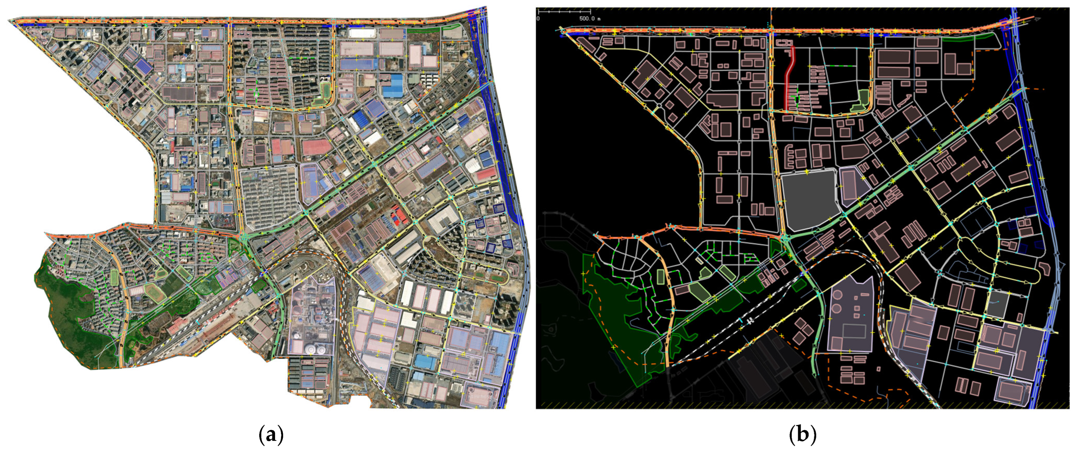
A high-accuracy baseline scenario was established first. The scenario was selected in an area of Dalian, China, which is an area around a frequently congested intersection with an area of 22 km² and a population of 71,018. Figure 1a shows the satellite map of this area. In the OSM, the directions of the roads are shown as arrows, and the buildings, mountains, and green areas are shown as polygons, as shown in Figure 1b.

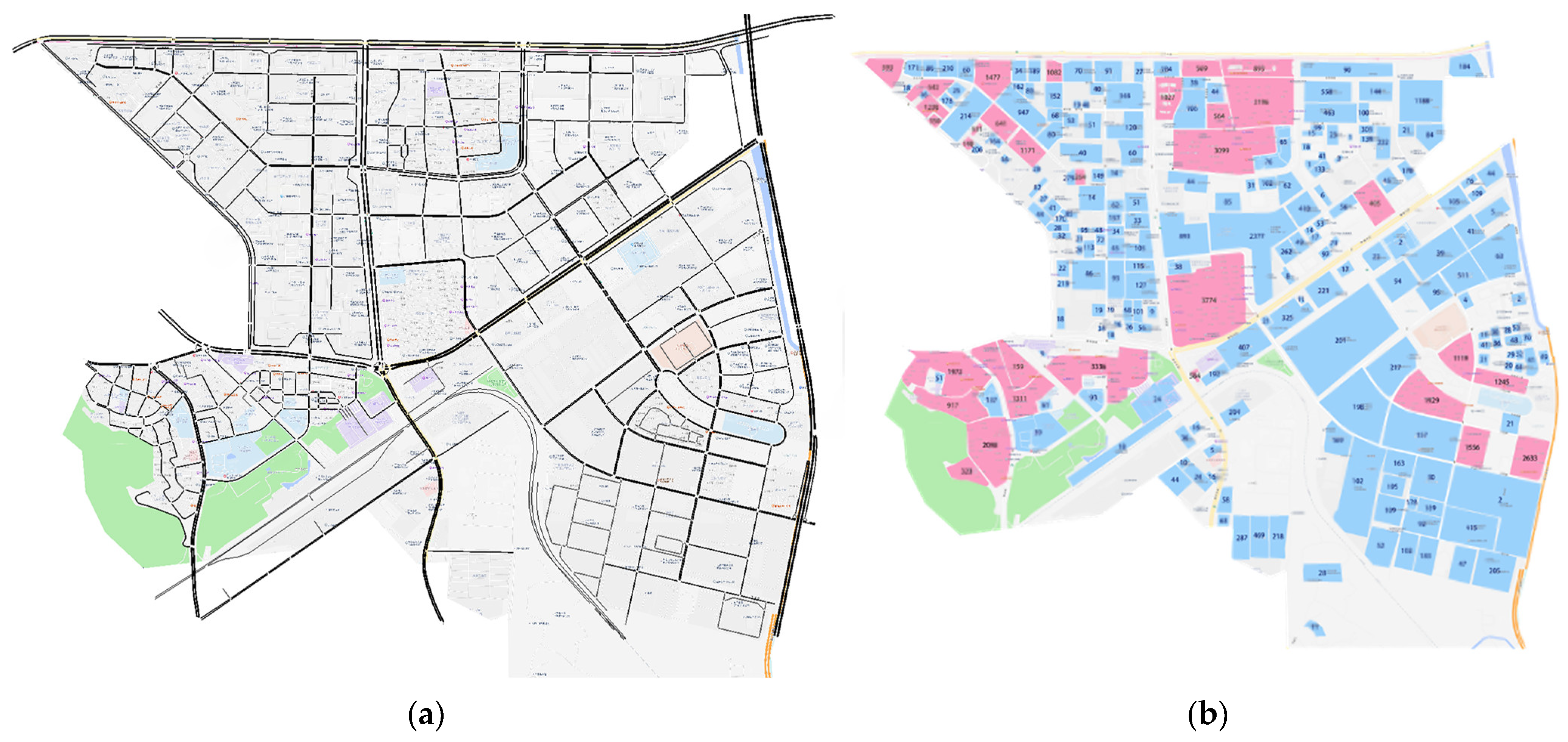
The road network data is imported from OSM into SUMO. The imported map was manually adjusted comparing the actual road conditions of each road section, and the adjusted map is shown in Figure 2a, where a screenshot of the map is used as a road network background. The manual adjustment of the road network will be introduced in detail in Section 2.2. Due to better data availability, traffic demand is generated from demographic geographic data. The core idea of using demographic geographic data to generate traffic demand is the commuting demand generated by people in this area going to and from work.

In SUMO, the sub-program ActivityGen generates traffic demand using demographic parameters including regional population, number of households, working hours distribution, car ownership rate, unemployment rate, age distribution, number of children and retirees, walking distance limits, and inbound/outbound traffic volume. It adjusts demand using parameters like car preference, average vehicle speed, leisure activity rate, random traffic parameters, and departure variables. ActivityGen distributes traffic demand across road segments within the area. In addition, if there is a number of residential areas and work locations on each road segment, ActivityGen can use this more precise data to generate more accurate traffic demand. This article compiled statistics on residential households (sourced from real estate websites) and workplaces locations/job numbers (sourced from company registered address and social security contributor counts). In Figure 2b, the residential areas (pink) are annotated with household numbers, and the workplaces (blue) with job numbers [31]. Traffic demand was allocated to road sections corresponding to the entrances and exits of these locations.

By default, vehicles select the fastest route under the assumption of being alone in the network. This may lead to unrealistic jamming and should be remedied with a traffic assignment method. In SUMO, the tool duaIterate.py can be used to compute the (approximate) dynamic user equilibrium. This script tries to find a route for each vehicle such that each vehicle cannot reduce its travel cost by using a different route. The number of iterations may be set to a fixed number of determined dynamically depending on the used options. For this scenario, 100 iterations were performed to identify the least congested routes for subsequent simulation.

To initially verify the traffic demand accuracy, a macroscopic-scale method (comparing map traffic conditions) was used. The AutoNavi map [32] is supported by AutoNavi Software Co., Ltd. (Beijing, China), which provides real-time traffic in three colors: red indicates congestion, with an average speed of less than 5 km/h, yellow indicated a low speed, with an average speed of 5–30 km/h, and green indicates smooth traffic, with an average speed over 30 km/h. The traffic data in the AutoNavi map were collected in real time from different sources: 15% of data were from the traffic control department of the city, and AutoNavi map users accounted for the remaining 85% of data. In most cities in China, AutoNavi cooperates with taxi companies to gain their floating car data (FCD). AutoNavi obtains FCD from each user while they are uploading their position during navigation. Through these sources, AutoNavi obtains real-time traffic data with high accuracy and fidelity.

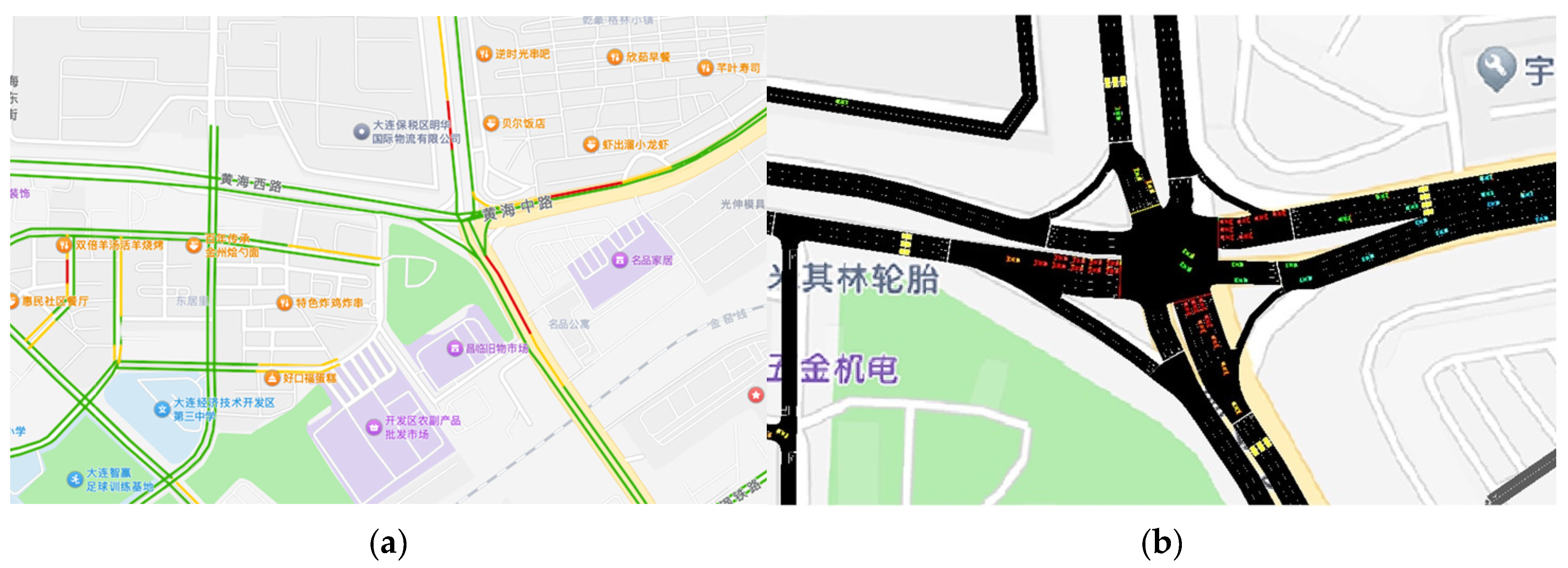
The most representative intersection in the simulation is selected to compare the traffic conditions, and its location is shown in Figure 3b, where the yellow rectangle is the inductive loops set in the simulation [31]. For the simulation data, the speed of the vehicles passing this verification point was recorded, and the data from multiple lanes on the same road section were averaged. For real-world data, the forecasted 24 h weekday traffic status from AutoNavi (based on historical same weekday, same-time data) was used. Figure 3a shows the forecasted traffic status of several road sections at 17:00 on Friday. As Figure 4 demonstrates, simulation results closely matched real weekday traffic conditions, indicating a persuasive scenario.

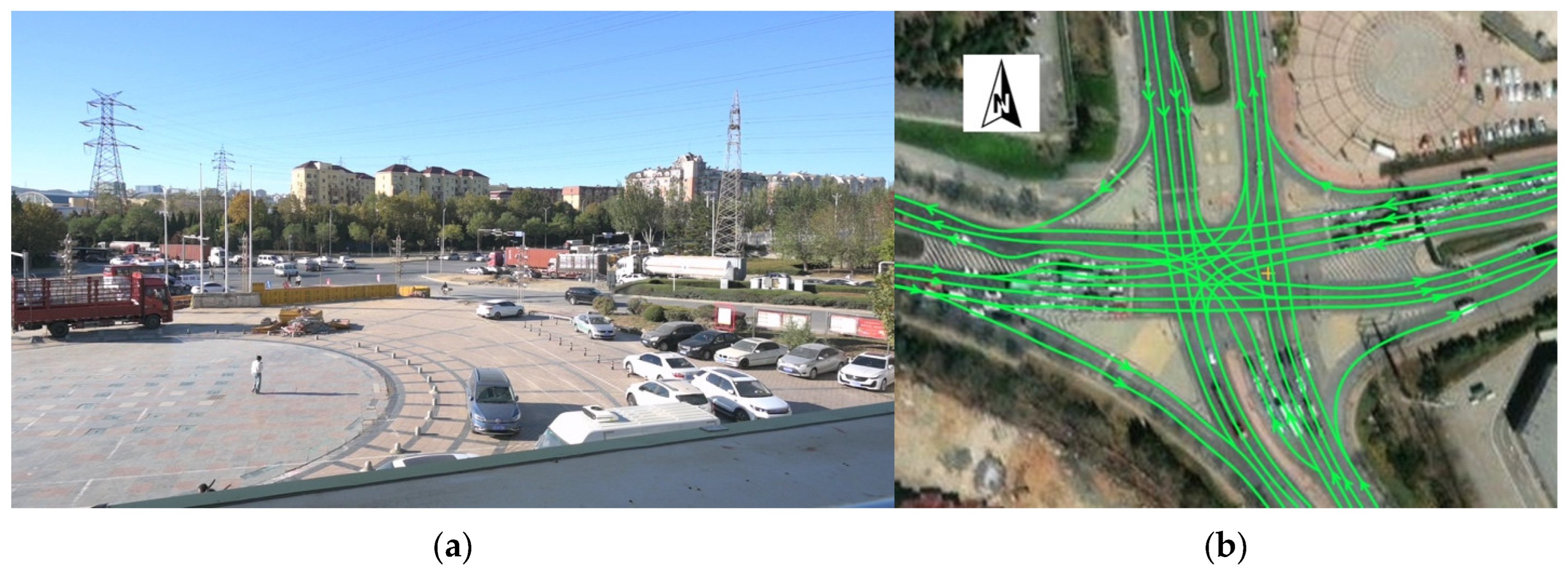
For precise accuracy verification, a microscopic method comparing traffic volume using camera data from the core intersection was employed. Figure 5 shows the intersection view and the road directions. Traffic at this intersection is complex and often congested during peak hours. Traffic flow was manually counted from video recordings during the morning (7:30–8:30) and evening (17:00–18:00) peaks on an ordinary weekday unaffected by weather, events, or holidays. Counted vehicles included passenger cars, buses, and light/heavy trucks. Bicycles, motorcycles, electric bicycles, and power-assisted tricycles were excluded, as they use separate lanes and minimally impact congestion. Vehicles passing per traffic light cycle in each driving direction were recorded in detail.

Simulated and real traffic flow of were categorized by origin directions (north, south, east, west). By adjusting work start/end time ratios, peak traffic volumes were calibrated to approximate real data (Figure 6). The RMSE (root mean square error) between the simulated and real vehicle counts at this intersection is 297.01.

2.2. Effect of Map Correction on Simulation Accuracy

Road networks from OSM often require manual correction in SUMO for inaccuracies like extra/missing road sections, wrong intersection connections, incorrect lane number/directions, wrong speed limits, permitted vehicle types, traffic light presence, etc. Manually correcting these errors by comparing with the corresponding street view map is time-consuming, limiting the area of the road network during simulation to a certain extent. This section investigates if this step can be omitted. The road network used here was imported from OSM with only basic connectivity adjustments, lacking detailed alignment with actual road conditions. Other simulation steps remained identical to the control group.

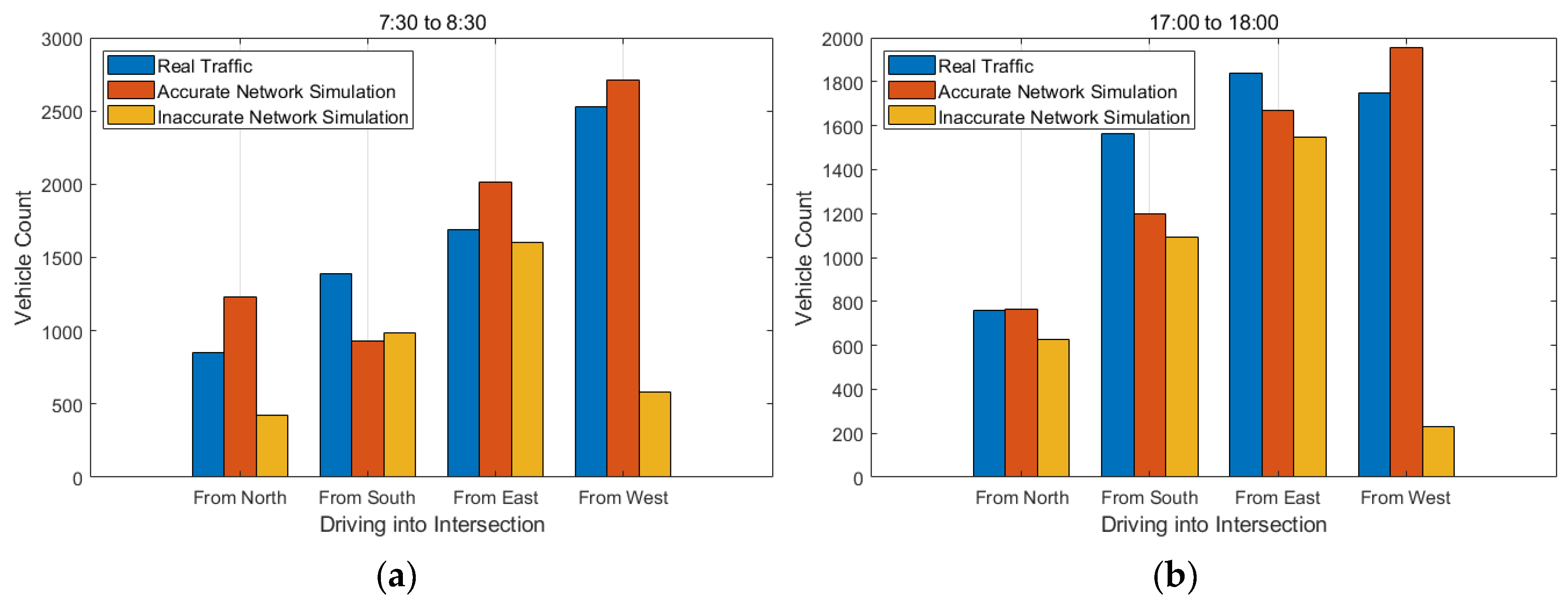
Figure 7 shows a significant decrease in vehicles passing the observation point under the same traffic demand—48% total reduction during the morning peak and 36% during the evening peak. These “missing” vehicles, which started from the origins were teleported to their destinations due to unrealistic congestion caused by the inaccurate road network. Thus, the precise road network crucially impact accuracy, with 42% of vehicles unable to travel along their original routes. The RMSE between simulation data without map correction and real data was 922.06. Compared to the RMSE of the corrected map simulation, the RMSE was 1024.53.

2.3. Effect of Traffic Data Generation on Simulation Accuracy

In the statistic file that generates traffic demand, the parameters that can be defined include the population of the area, age groups, working time ratio, number of residents and jobs on each street, number of schools and students, bus stops and routes, etc. In these parameters, schools and buses are optional. The simulation area contains 16 kindergartens, 4 primary schools, and 3 middle schools. If these schools are not defined, the number of trips will be reduced by 0.37% in the simulation. The area also has 34 pairs of bus stops and 13 bus routes. If bus routes are not defined, the number of trips will increase by 47%. Thus, defining schools has minimal impact, whereas omitting bus routes significantly increases traffic volume (primarily private cars).

2.4. Effect of Simulation Iterations on Simulation Accuracy

In SUMO, the logic of route planning is to use the shortest route method, that is, after all vehicles have specified the origin–destination relations (trips), the simulation determines routes through the network (list of edges) by computing the shortest or fastest routes. This will result in an unrealistic uneven assignment of users. For example, two parallel roads may have no cars on the longer road because one road is only 2 m longer than the other. In SUMO, this problem is solved using an iterative assignment called DUE (Dynamic User Equilibrium). Iterating an assignment to find the shortest travel times for all vehicles is not very laborious, but it is very time consuming. Is this work that can be omitted?

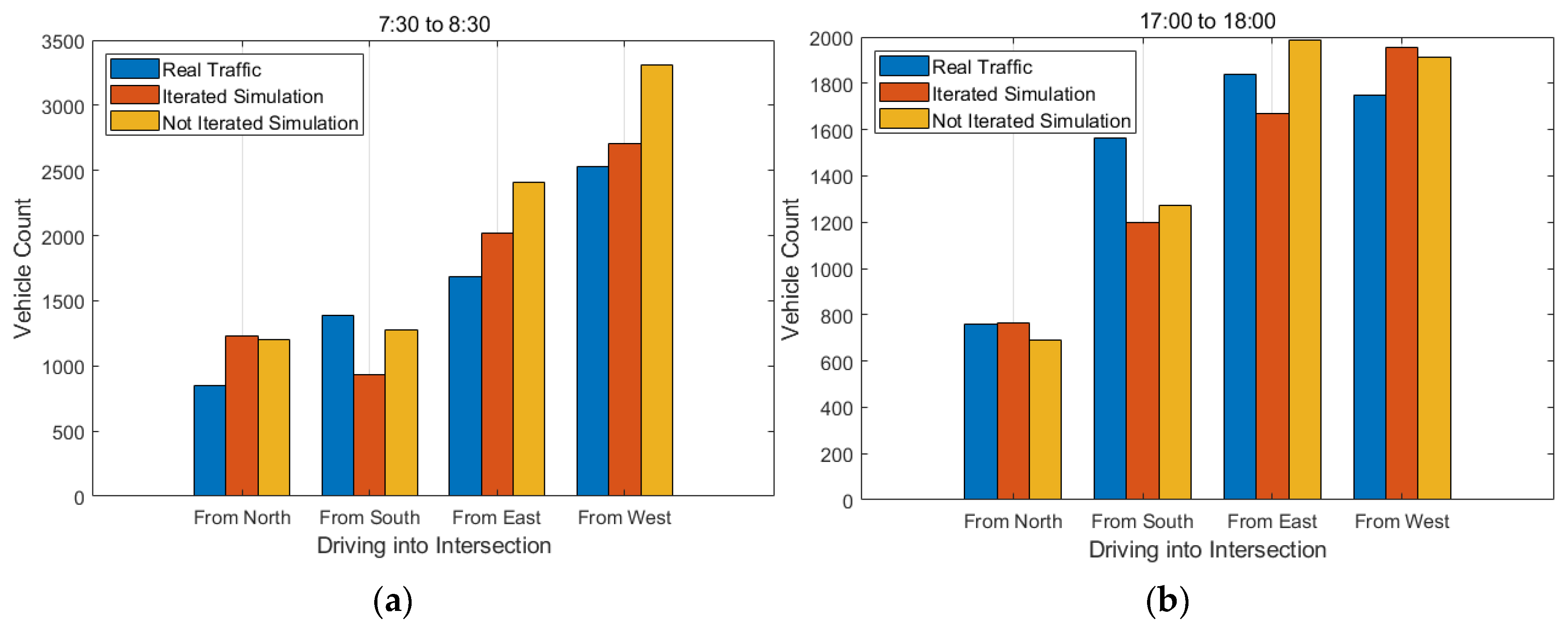
Figure 8 compares non-iterated routes and optimal routes after 100 iterations. As can be seen from the figure, non-iterated routes unrealistically increased vehicle counts at the observation point by 13% compared to iterated routes, as the shorter path concentrated through this point. Teleported vehicles due to congestion and other factors in the non-iterated routes simulation is 624 times that of the iterated routes, accounting for 6.6% of the total number of vehicles. Iterations significantly improve the traffic conditions. The RMSE between the number of vehicles simulated using non-iterated data and the real data is 418.85, while the RMSE between the number of vehicles simulated using non-iterated data and the optimal data after 100 iterations is 305.96.

2.5. Effect of Using Actual Traffic Lights on Simulation Accuracy

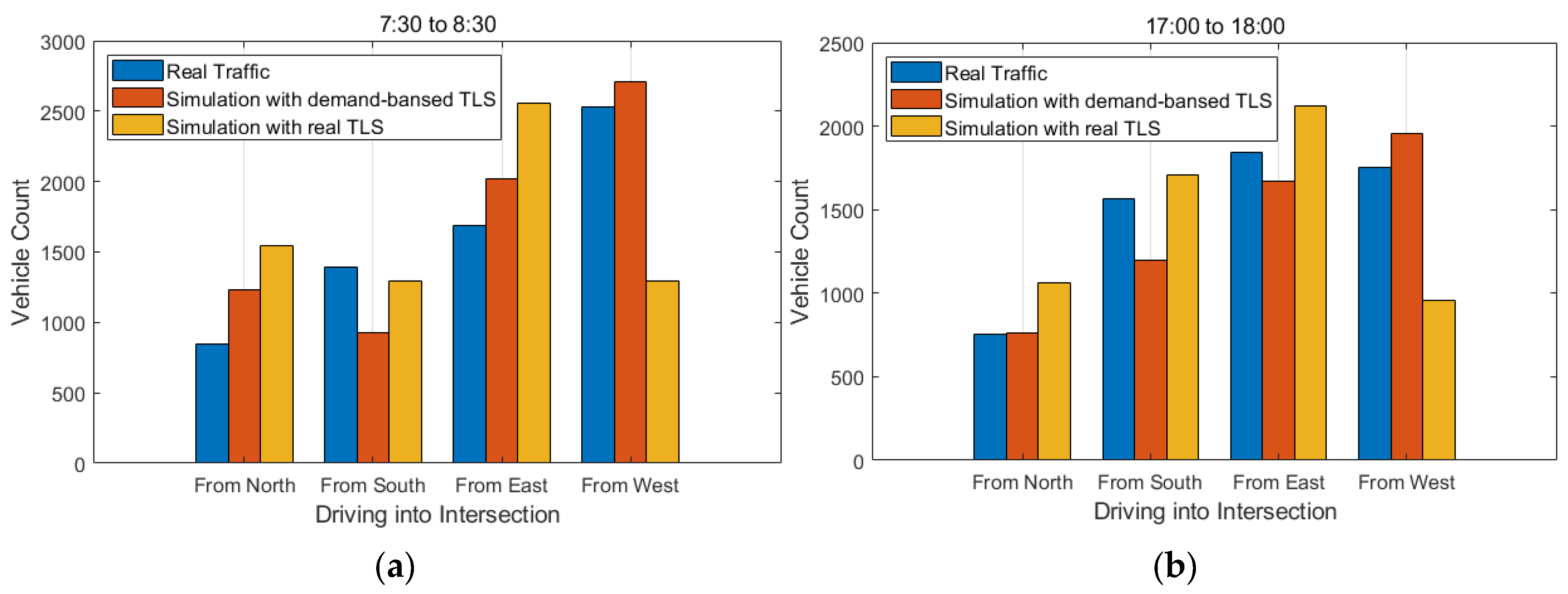
Figure 9 compares vehicle counts using real traffic light systems (TLS), demand- based default TLS, and the real traffic flow. Although overall traffic volume differences were small, the junction turning percentage, that is, the distribution ratio of straight, left, and right turns is quite different from the real road conditions. For instance, for vehicles entering the intersection from the west, the simulation had more left-turning vehicles, whereas reality had more going straight. Consequently, using real TLS for the simulation model caused significant congestion in specific directions. The RMSE between simulation using real TLS and real data was 670.81, while the RMSE between simulations using real TLS and default TLS was 713.73.

3. Discussion

Controlling different simulation parameters revealed their varying impacts on simulation accuracy. Map correction (Section 2.2) and route iteration (Section 2.4) significantly affect results. Uncorrected OSM and non-iterated routes cause unrealistic traffic congestion, substantially reducing simulation accuracy. The impact of including school and bus route information in traffic demand also differed markedly. Adding schools increased total traffic volume by 0.37%, whereas undefined bus routes increased it by 47%, profoundly impacting accuracy.

Factors significantly impacting the simulation accuracy include map correction, route iteration, and using real-world TLS. The RMSE values for these factors were higher than the control group’s RMSE (297.01). The most significant effect came from the uncorrected map (RMSE = 922.06), while the effect of non-iteration is smaller (RMSE = 418.85). The pronounced impact of uncorrected maps likely stems from disconnected roads causing widespread unrealistic congestion affecting the entire area. In contrast, non-iteration congestion arises from vehicles all choosing the shortest-distance route instead of the shortest-time route, overloading some roads while underutilizing alternatives.

Theoretically, using real TLS should enhance accuracy, but our results showed increased error (RMSE = 670.81). This is likely because the turning percentage distribution in the simulation differed from reality, causing the real TLS timing to be maladapted to the simulation traffic flow, negatively impacting simulation accuracy.

4. Conclusions

This study investigated factors affecting microscopic traffic simulation accuracy by controlling various parameters. It successfully reconstructed urban traffic conditions with high fidelity (RSME = 297.01) using real road data and Internet-sourced information, validated through both macroscopic and microscopic methods. This work offers valuable insights for future traffic simulation development.

Among the factors studied, uncorrected maps had the greatest negative impact (RSME = 922.06), followed by using real traffic light data (RSME = 670.81), and non-iterated routes (RSME = 418.85). Defining school zones had negligible impact. When generating traffic demand using demographic population data, omitting bus routes increased private car trips by 47%, significantly exacerbating congestion.

For researchers prioritizing efficiency during the scenario setup:

• Manual map correction is essential.
• When using demographic population data to generate traffic demand, defining bus routes is crucial to maintain accuracy.
• Route iterations can potentially be omitted if accuracy requirements are moderate, saving computational time.
• Incorporating real traffic light data is not recommended unless the simulated turning percentages closely match reality, as it can be counterproductive.
• For general areas (not school-dense), excluding school definitions has minimal impact and can be omitted.

Building upon accurate maps, future work will investigate other influencing factors such as different vehicle types, driver behaviors, and the impact of autonomous vehicles on traffic.