Article

Hybrid Frequency–Temporal Modeling with Transformer for Long-Term Satellite Telemetry Prediction

1
National Space Science Center, Chinese Academy of Sciences, Beijing 100190, China
2
Department of Computer Science and Technology, University of Chinese Academy of Sciences, Beijing 101408, China
*
Author to whom correspondence should be addressed.
Appl. Sci. 2025, 15(21), 11585; https://doi.org/10.3390/app152111585
Submission received: 18 September 2025 / Revised: 16 October 2025 / Accepted: 27 October 2025 / Published: 30 October 2025

Abstract

Reliable forecasting of satellite telemetry is critical for spacecraft health management and mission planning. However, conventional data-driven methods often struggle to effectively capture both the long-term dependencies and local dynamics inherent in telemetry data. To tackle these challenges, we introduce FFT1D-Dual, a hybrid Transformer framework that unifies frequency-domain and temporal-domain modeling, effectively capturing both long-term dependencies and local features in telemetry data to enable more accurate satellite forecasting. The encoder replaces computationally expensive self-attention with a novel Dual-Path Mixer encoder that combines one-dimensional Fast Fourier Transform (FFT) and temporal convolutions, adaptively fused via a learnable channel-wise gating mechanism. A standard attention-based decoder with dynamic positional encodings preserves temporal reasoning capability. Experiments on real-world satellite telemetry datasets demonstrate that FFT1D-Dual mostly outperforms baselines across both short- and long-term horizons across three representative telemetry variables while maintaining consistently lower error growth in long-horizon predictions. Ablation studies confirm that the combination of frequency-domain modeling and dual-path fusion jointly contributes to these gains. The proposed approach provides an efficient solution for accurate long-term forecasting in complex satellite telemetry scenarios.

1. Introduction

With the increasing complexity of space missions, accurate and timely forecasting of satellite telemetry has become a critical prerequisite for on-board system monitoring, fault prevention, and autonomous decision-making [1]. Telemetry signals are collected from multiple subsystems such as power distribution, thermal control, and sensor feedback, and exhibit highly diverse temporal dynamics characterized by non-stationary trends, abrupt transitions, and pronounced long-term dependencies [2]. Among these properties, effectively modeling long-term dependencies remains the most challenging task: on the one hand, telemetry data often span extremely long time scales, where crucial state evolutions occur sparsely and in subtle positions across sequences; on the other hand, local perturbations and noise can amplify prediction errors and accumulate over time, making it difficult for models to maintain stable accuracy across long forecasting horizons [3,4]. Consequently, the ability to capture and leverage long-range dependency structures efficiently has become a central challenge in satellite time series forecasting research.
In the field of satellite telemetry time series forecasting, Recurrent Neural Network (RNN)-based methods remain mainstream. For instance, Neto et al. (2025) proposed integrating GAN and BiLSTM for multidimensional telemetry forecasting in the context of digital twins [5]. Lin and Junyu (2025) applied LSTM networks for satellite orbit prediction based on Two-Line Element data [6]. Guo et al. (2025) proposed the BiLSTM-TS model for medium-orbit satellite orbit prediction [7]. Kricheff et al. (2024) applied explainable methods to LSTM and a hybrid IF-CBLOF model for anomaly detection in satellite telemetry data [8]. Xu et al. (2024) proposed a hybrid Monte Carlo quantile EMD-LSTM method for satellite in-orbit temperature prediction and uncertainty quantification [9]. Knap et al. (2024) used a LSTM network to predict solar power for controlling charging current and extending battery life in CubeSats [10]. Peng et al. (2024) proposed an Attention-BiLSTM model leveraging telemetry correlations for accurate satellite operation predictions [11]. Xu et al. (2023) developed a multivariate anomaly detector for satellite telemetry using a temporal attention-based LSTM autoencoder [12]. Wang et al. (2022) proposed a deep learning framework for satellite telemetry anomaly detection using synthetic anomalies [13]. Zeng et al. (2022) proposed an anomaly detection method for satellite telemetry using a causal network and feature-attention-based LSTM [14]. Yang et al. (2021) developed an improved deep learning approach for telemetry anomaly detection to enhance spacecraft operation reliability [15]. Tao et al. (2021) proposed a GRU-GARCH and MD hybrid method for long-term satellite degradation prediction using heteroscedastic telemetry data [16].
In addition to RNN-based models, Convolutional Neural Network (CNN)-based methods have also been explored for satellite telemetry prediction and anomaly detection. Gallon et al. (2025) proposed a multi-channel CNN for detecting and isolating “stuck” sensor values in accelerometers and IMUs of SSSB exploration spacecraft [17]. Tang et al. (2024) introduced an unsupervised anomaly detection framework combining Graph Attention Networks (GATs) and TCNs for continuous monitoring of ACS telemetry [18]. Zeng et al. (2022) proposed a Causal Multivariate Temporal Convolutional Network (CMTCN), which first constructs a causal graph using Anomalous Transfer Entropy (ATE) and then applies a multi-feature Temporal Convolutional Network (TCN) for data prediction [19].
Traditional forecasting methods, including RNNs (e.g., GRU and LSTM) and temporal CNNs, often struggle with long-term accuracy: RNNs can capture short-term dependencies but suffer from vanishing gradients and error accumulation over long horizons, while temporal CNNs efficiently model local patterns but have limited receptive fields for long-range dependencies [20,21].
Recently, Transformer-based models have demonstrated strong performance on time series forecasting tasks, owing to their parallelism and long-range attention [22,23,24,25]. Qiao et al. (2025) proposed TEMPO, a time-evolving multi-period method for anomaly detection in space probe data [26]. Song et al. (2025) applied a Transformer-based model for time series forecasting of telemetry data in spacecraft environmental control and life support systems [27]. Park and Yun (2025) proposed a data-driven method for estimating battery degradation in low-Earth-orbit satellites [28]. Gao et al. (2025) proposed a lightweight Transformer enhanced with FastDTW for fault warning in satellite momentum wheels [29]. Zhao et al. (2024) developed an advanced Transformer architecture for early anomaly detection in non-stationary satellite telemetry data [30]. Lan et al. (2024) proposed a fault prediction method for satellite rotating mechanisms using SSA and an improved Informer model [31].
However, Transformer models suffer from a computational cost that scales quadratically with sequence length. This scaling issue not only increases memory consumption and training time but also limits their practicality when handling large-scale telemetry datasets, where both efficiency and responsiveness are critical [32].
To address these limitations, we introduce FFT1D-Dual, a novel Transformer architecture that fuses frequency-domain modeling and temporal-domain convolution within a dual-path encoder. Our design departs from the conventional reliance on self-attention in the encoder by leveraging a 1D Fast Fourier Transform (FFT) to capture periodic and global structures, and a 1D convolution to model local variations. These two representations are adaptively fused through a channel-wise gating mechanism, enabling the model to learn modality preference per feature. The decoder follows a standard Transformer configuration, augmented with learnable dynamic positional encodings to enhance temporal sensitivity. Our contributions are threefold:
  • We propose a new Transformer architecture with a frequency-aware hybrid encoder, eliminating attention from the encoder and enabling efficient modeling of both global periodicity and local transitions.
  • We introduce a Dual-Path Mixer with a channel-wise fusion gate, allowing adaptive time–frequency fusion at the feature-channel granularity.
  • We conduct extensive experiments on real satellite telemetry data, demonstrating significant improvements over baseline models in terms of forecasting accuracy, stability, and scalability, especially on long-term horizons.

2. Methods

2.1. Method Overview

2.1.1. Data Processing

We propose a time series forecasting framework specifically designed for satellite telemetry data as shown in Figure 1, comprising two main components: data preprocessing and the prediction model. In our case, we use delayed telemetry from the EP satellite power subsystem, sampled every 30 s, which includes 69 multivariate features from various subsystems, including power system diagnostics (e.g., bus voltages and battery currents), component-specific telemetry (e.g., sensor voltages), and thermal control indicators (e.g., internal temperatures). A representative summary is provided in Table 1.
The raw telemetry data are reorganized according to feature type, where either a single target variable (S), multiple variables (M), or multiple-to-single mapping (MS) is considered. Let the dataset be denoted as
D = { ( x t , y t , τ t ) } t = 1 T ,
where x t R d represents the multivariate features at time t, y t R is the target variable, and τ t denotes the timestamp. The telemetry data are first processed through a standard preprocessing pipeline. The dataset is then partitioned chronologically into training, validation, and test subsets with proportions of 0.7:0.1:0.2:
D = D train D val D test , | D train | : | D val | : | D test | = 7 : 1 : 2 .
For each feature dimension j { 1 , , d } , the mean and variance are computed on the training set:
μ j = 1 | D train | ( x , y , τ ) D train x ( j ) , σ j 2 = 1 | D train | ( x , y , τ ) D train x ( j ) μ j 2 .
All features are standardized as
z t ( j ) = x t ( j ) μ j σ j .
Using a sliding-window mechanism, each training instance consists of the following:
Input sequence:
X = ( x t , x t + 1 , , x t + L 1 ) , X R L × d ,
where L is the input length.
Output sequence:
Y = ( y t + L , , y t + L + H 1 ) , Y R H ,
where H is the forecasting horizon.
Thus, the dataset for model training can be expressed as
S = { ( X i , Y i , τ i ) } i = 1 N .
Timestamps τ t are preserved as auxiliary covariates and extrapolated for future steps under the assumption of a uniform sampling interval Δ τ .

2.1.2. Model Architecture

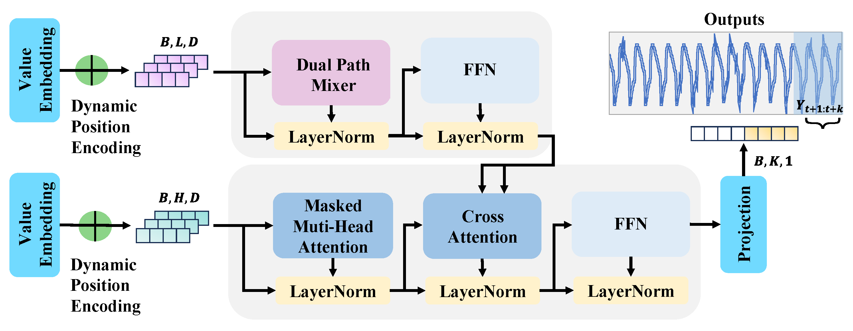
The proposed FFT1D-Dual, a hybrid forecasting framework that integrates frequency-domain modeling with attention mechanisms. The architecture consists of three major components: (i) a Dual-Path Mixer (DPM)-based encoder combining Fourier and convolutional operations; (ii) a standard Transformer-based decoder; (iii) a learnable dynamic positional encoding module. As illustrated in Figure 2, the encoder leverages the proposed DPM to jointly capture temporal and frequency-domain dependencies, effectively reducing the reliance on traditional self-attention layers.
Given a multivariate time series
X = ( x t , x t + 1 , , x t + L 1 ) , X R L × d ,
where L is the input length and d is the feature dimension, the corresponding target sequence is defined as
Y = ( y t + L , , y t + L + H 1 ) , Y R H ,
The input sequence X is first projected into a hidden space of dimension D:
X ˜ = Linear ( X ) + P , X ˜ R B × L × D ,
where B denotes the batch size and P is the learnable dynamic positional encoding.
The encoder applies a Dual-Path Mixer to capture temporal and spectral dependencies. Formally, for each hidden representation X ˜ , we compute
F = F ( X ˜ ) , X ^ f = ϕ f ( F ) ,
where F denotes the one-dimensional Fourier Transform, and ϕ f is a frequency-domain filter. Meanwhile, a temporal convolutional operation is applied:
X ^ t = ϕ t ( X ˜ ) ,
where ϕ t represents a depthwise convolution capturing local temporal patterns. The outputs are fused as
Z = α · X ^ f + ( 1 α ) · X ^ t ,
where α is a learnable gating parameter. This design allows the encoder to capture both global periodicity (via X ^ f ) and local variations (via X ^ t ).
The decoder follows the standard attention-based design. Given the encoder representation Z and the autoregressively masked target embedding Y ˜ R B × H × D , the decoder applies multi-head attention:
DecOut = TransformerDecoder ( Y ˜ , Z ) .
Finally, the prediction is obtained by projecting into the target space:
Y ^ = W o · DecOut + b o , Y ^ R B × H .
The model generates predictions of horizon length H, i.e.,
Y ^ = ( y ^ t + L , y ^ t + L + 1 , , y ^ t + L + H 1 ) ,
which correspond to the forecasted values of the target variable.
The proposed method offers several advantages: (1) Efficiency: The encoder eliminates quadratic self-attention, reducing computational cost. (2) Adaptability: Dual-path fusion enables dynamic learning of both spectral and temporal patterns. (3) Long-term forecasting capability: Frequency-domain modeling captures periodicity and long-range dependencies, making FFT1D-Dual especially effective for mid- to long-term forecasting tasks.

2.2. DPM-Based Encoder

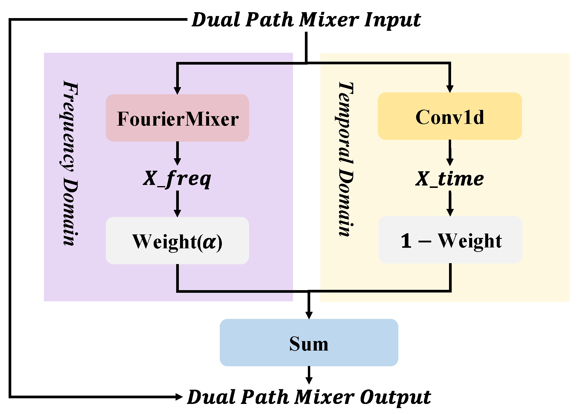
To effectively integrate both local and global patterns in sequential data, we propose a Dual-Path Mixer(DPM), as illustrated in Figure 3. The module consists of four main components: (1) a frequency-domain path based on the Fourier transform; (2) a temporal convolution path; (3) a channel-wise gating mechanism for adaptive fusion; (4) residual connections with feedforward layers to enhance stability and nonlinear modeling capacity.

2.2.1. Parallel Frequency and Temporal Paths

Given an input sequence
X R B × L × D ,
where B is the batch size, L the sequence length, and D the feature dimension; the data is processed in parallel along two paths:
Frequency path:
X freq = FourierMixer ( X ) , X freq R B × L × D ,
where the FourierMixer applies a Fast Fourier Transform (FFT) along the temporal axis and a learnable complex-valued projection to extract spectral representations.
Temporal path:
X time = Conv 1 D ( X ) , X time R B × L × D ,
where a one-dimensional convolution captures local temporal dependencies.

2.2.2. Channel-Wise Gating Fusion

Rather than applying a uniform fusion strategy, we introduce a channel-wise gating mechanism that adaptively balances the contribution from frequency and temporal features. Specifically, a learnable parameter vector
α R D
is applied channel-wise and passed through a sigmoid activation:
w = σ ( α ) , w ( 0 , 1 ) D .
The fused representation is then computed element-wise as
X fused [ : , : , d ] = w d · X freq [ : , : , d ] + ( 1 w d ) · X time [ : , : , d ] , d = 1 , , D .
This formulation enables each feature channel to independently adjust its reliance on frequency-domain information (e.g., periodic or global patterns) versus temporal-domain information (e.g., local transitions or abrupt changes).

2.2.3. Residual Enhancement

To promote gradient flow and stabilize training, we employ a residual connection:
Y = X fused + X ,
where Y R B × L × D serves as the output of the fusion module.

2.2.4. Advantages

Compared to fixed or globally shared fusion strategies, the proposed channel-wise fusion provides fine-grained adaptability across heterogeneous time series channels. This improves representational flexibility and allows the model to dynamically adjust to diverse temporal dynamics. Moreover, the learned gating weights w offer interpretable insights into the relative importance of spectral versus temporal information, which is particularly valuable in applications such as satellite telemetry forecasting and multivariate time series modeling.

2.3. Fourier Mixer Module

The proposed Fourier Mixer Module (FMM), illustrated in Figure 4, serves as the core component for the frequency-domain path within the Dual-Path Mixer (Section 2.2). It introduces a one-dimensional Fast Fourier Transform to efficiently capture spectral representations. This module focuses solely on the frequency-domain transformation. Its output is subsequently sent to the channel-wise gating mechanism of the Dual-Path Mixer (Section 2.2) for fusion with the temporal path.

2.3.1. Fourier Transform Path

Given an input sequence
x R B × L × D ,
where B denotes the batch size, L the sequence length, and D the feature dimension, a one-dimensional Fourier transform is applied along the temporal axis:
X fft = F t ( x ) = FFT ( x , dim = 1 ) , X fft C B × L × D .
This produces a complex-valued representation encoding frequency components of the input signal. To fully utilize both the real and imaginary parts, we introduce a complex projection mechanism, which applies independent linear projections:
Real = W r · ( X fft ) ,
Imag = W i · ( X fft ) ,
where W r , W i R D × D are learnable projection matrices. The frequency-domain representation is then reconstructed as
X out = Real + Imag , X out R B × L × D .
This learnable complex-domain projection enables flexible transformations of spectral features, enhancing the model’s capacity to capture long-term periodicity and non-stationary dynamics.

2.3.2. Temporal Convolution Path and Fusion

In parallel, a temporal convolution path is applied:
X time = Conv 1 D ( x ) .
The outputs of the frequency and temporal paths are fused using the channel-wise gating mechanism (see Equation (11)), producing the final representation X fused .

2.3.3. Complexity Analysis and Advantages

Unlike conventional convolutional or attention-based mechanisms, the Fourier Mixer operates in the frequency domain with a computational complexity of
O ( L log L ) ,
which is significantly more efficient than self-attention O ( L 2 ) for long sequences. Moreover, frequency-domain modeling inherently provides stronger global representation capacity by capturing periodic structures and long-range dependencies. This makes the Fourier Mixer Module both computationally efficient and highly effective for long-term forecasting tasks, while maintaining stability and spectral fidelity.

2.4. Decoder and Attention Mechanisms

In contrast to the encoder, which eliminates self-attention, the decoder retains the standard Transformer-style attention architecture to preserve strong temporal reasoning capability. Each decoder layer consists of three sub-blocks: self-attention, cross-attention, and a feedforward network (FFN), with residual connections and normalization applied to enhance stability.
The core operation is the Scaled Dot-Product Attention, defined as
Attention ( Q , K , V ) = Softmax Q K d k V ,
where Q , K , V R B × L × d k denote query, key, and value matrices, and d k is the key dimension. This mechanism enables the decoder to model temporal dependencies while preventing information leakage via causal masking in the self-attention block, and to align predictions with encoder outputs via cross-attention.
To further enrich representational capacity, we employ Multi-Head Attention, which projects Q , K , V into h subspaces and performs attention in parallel:
head i = Attention ( Q W i Q , K W i K , V W i V ) ,
MHA ( Q , K , V ) = Concat ( head 1 , , head h ) W O .
Finally, the decoder output X dec R B × K × D is projected to the forecasting target dimension through a linear mapping:
Y ^ = Linear ( X dec ) R B × K × 1 ,
where K is the prediction horizon. This projection aligns the learned high-dimensional representations with the target variable space, producing the final forecasting results.
Overall, by retaining attention mechanisms in the decoder, the model preserves strong expressive power to capture complex temporal dependencies and align encoder representations with forecasting tasks.

2.5. Dynamic Positional Encoding

To effectively incorporate temporal order into the model, we introduce a Dynamic Positional Encoding (DPE) module. Given the input sequence
X R B × L × d model ,
we define a learnable positional embedding matrix
P R 1 × L max × d model ,
where L max is the maximum sequence length and d model is the hidden dimension.
Unlike fixed sinusoidal encodings, DPE introduces a learnable channel-wise scaling vector
γ = [ γ 1 , γ 2 , , γ d ] R d , γ i [ 0 , 1 ] ,
which adaptively controls the contribution of each positional channel. The dynamic positional embedding is computed as
P ˜ ( : , t , i ) = P ( : , t , i ) · γ i , for t = 1 , , L , i = 1 , , d .
Finally, the encoded input is obtained by combining token representations with the dynamic positional embeddings:
X enc = X + P ˜ .
This design allows the model to dynamically adjust the relative importance of positional information across different feature channels, enabling better adaptation to diverse temporal dynamics compared to fixed or fully learnable positional embeddings.

3. Results

3.1. Dataset Description

The dataset employed in this study consists of delayed telemetry data collected from the EP satellite over a continuous 24 h period in January. The raw telemetry was sampled at 1 s intervals, resulting in 86,400 records. To mitigate redundancy and improve modeling efficiency, we downsampled the data to a 30 s interval, yielding
N = 86,400 30 = 2880
time steps.
The dataset contains 69 multivariate features encompassing various satellite subsystems, including the following:
  • Power system diagnostics: multiple bus voltages, battery voltages, and current readings;
  • Component-specific telemetry: sensor voltages (e.g., star sensor, gyroscope);
  • Thermal control indicators: internal temperatures from distributed sensors.
This heterogeneous dataset presents significant challenges due to its temporal complexity, non-stationary behavior, and the diversity of subsystem signals.
Table 1 provides a representative summary of selected variables, including their names, units, and subsystem categories. This facilitates interpretation by linking raw telemetry parameters to their physical meaning in satellite operation.

3.2. Experimental Settings

To evaluate the effectiveness of the proposed FFT1D-Dual model, we conduct a series of multivariate time series forecasting experiments on satellite telemetry data. The forecasting task is formulated under a multivariate-to-univariate (MS) setup, where all 69 features are used as input, while a single target variable is predicted. Specifically, three representative telemetry parameters—TMD11, TMD12 and TMD74—are selected as forecasting targets.

3.2.1. Model Configuration

The architectural configuration of FFT1D-Dual is summarized in Table 2. The encoder employs a frequency-enhanced Dual-Path Mixer in place of the standard self-attention mechanism, while the decoder retains the Transformer architecture with scaled dot-product attention and a multi-head design. Both encoder and decoder adopt dynamically learnable positional encodings.

3.2.2. Sequence Setup

To evaluate performance across different forecasting horizons, we configure dynamic prediction settings with the prediction length L pred varying from 1 to 100 (step size = 1 ). For each prediction step, the decoder label length is set equal to the prediction length:
L label = L pred ,
and the input sequence length is set to twice the prediction length:
L input = 2 × L pred .
This proportional setup ensures a consistent ratio of historical context to prediction target across all settings, enabling fair performance comparison under different temporal spans.

3.2.3. Evaluation Metrics

We adopt two widely used regression metrics: Mean Squared Error (MSE) and Mean Absolute Error (MAE). They are formally defined as follows:
MSE = 1 n i = 1 n y i y ^ i 2 , MAE = 1 n i = 1 n | y i y ^ i | ,
where y i and y ^ i denote the ground truth and predicted values, respectively. MSE penalizes larger deviations more severely, reflecting overall prediction accuracy, while MAE provides an intuitive measure of average prediction error magnitude. These metrics are computed on the test set for each prediction horizon, with lower values indicating better forecasting performance.
While RMSE is a widely used metric, it is mathematically correlated with MSE and was omitted to avoid redundancy; MSE and MAE together could provide a complementary and sufficient assessment of prediction accuracy and error distribution.

3.2.4. Hardware and Implementation

All experiments were conducted using the PyTorch 2.1.0 deep learning framework with Python3.8.20. The detailed hardware and software configurations are summarized in Table 3.

3.3. Comparison with Baselines

3.3.1. Quantitative Evaluation of Forecasting Performance

To comprehensively evaluate the effectiveness of the proposed approach, we benchmark our model against several representative baselines, including GRU, LSTM, and TCN. The comparison is conducted on three telemetry variables (TMD11, TMD12, and TMD74), with prediction horizons ranging from 1 to 100 steps. Forecasting performance is assessed using two widely adopted regression metrics: Mean Squared Error (MSE) and Mean Absolute Error (MAE).
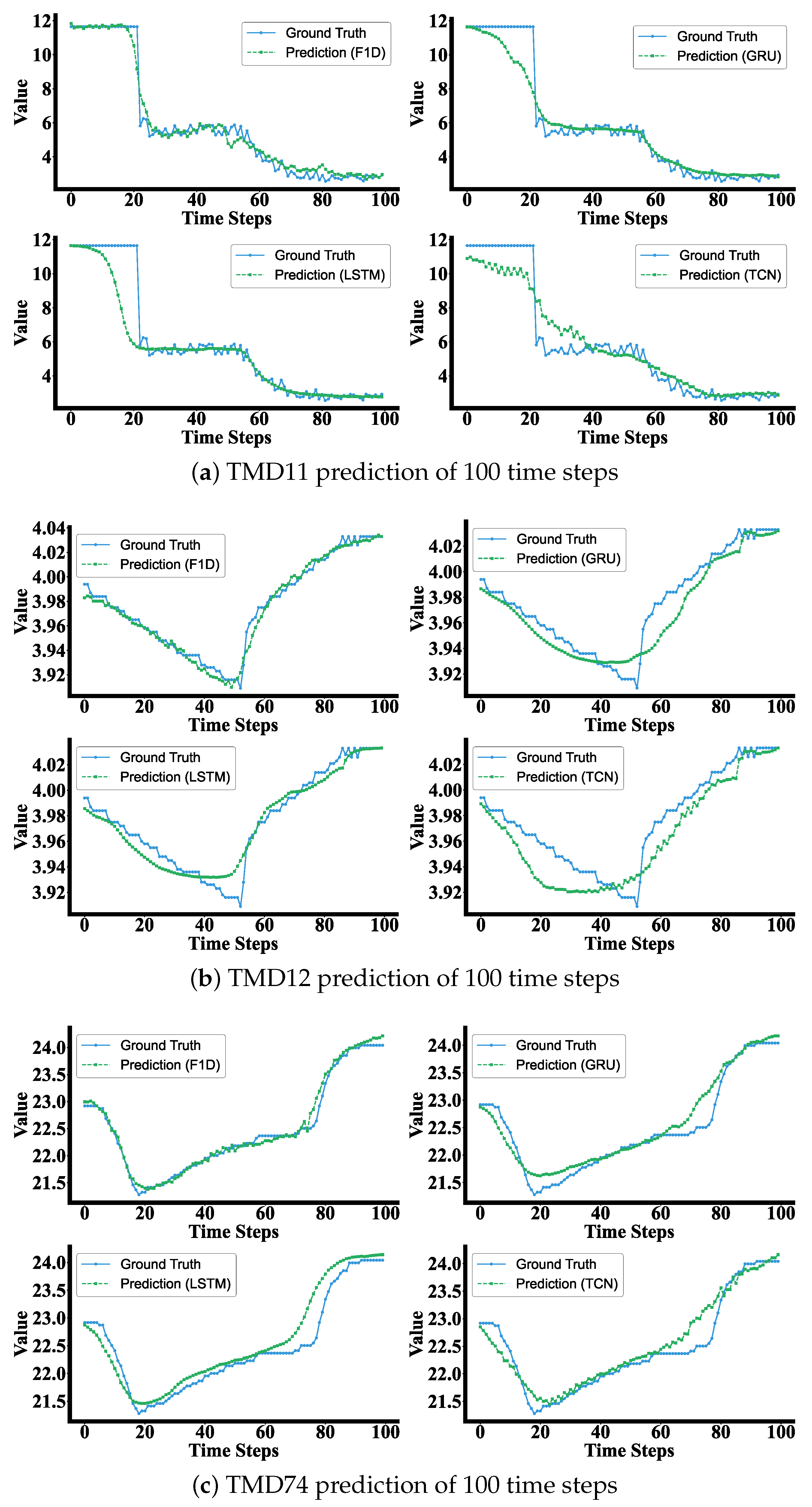
As reported in Table 4, Table 5 and Table 6 and illustrated in Figure 5, which shows one-shot predictions for individual representative samples, the proposed FFT1D-Dual (hereafter referred to as F1D), consistently outperforms the baseline methods across most horizons and target variables. On TMD11, where the telemetry exhibits irregular and delayed variations, F1D delivers more stable and accurate forecasts compared to GRU, LSTM, and TCN, particularly for long-range horizons. On TMD12, which is characterized by smooth fluctuations and a narrow numerical range, F1D still achieves the lowest error values across all horizons, demonstrating robustness on low-variance signals. On TMD74, F1D achieves substantially lower MSE and MAE in both short-term (1–10 steps) and long-term (60–100 steps) forecasts, highlighting its capability to capture both abrupt changes and gradual temporal trends.
The line plots in Figure 5 visualize the predicted trajectories overlaid with ground truth signals for representative cases. It is evident that F1D produces predictions that closely follow the actual patterns, with reduced phase shifts and improved amplitude alignment. Collectively, these results demonstrate that the proposed frequency-aware architecture yields more accurate and stable forecasting performance than conventional sequence models.

3.3.2. Error Curve Analysis

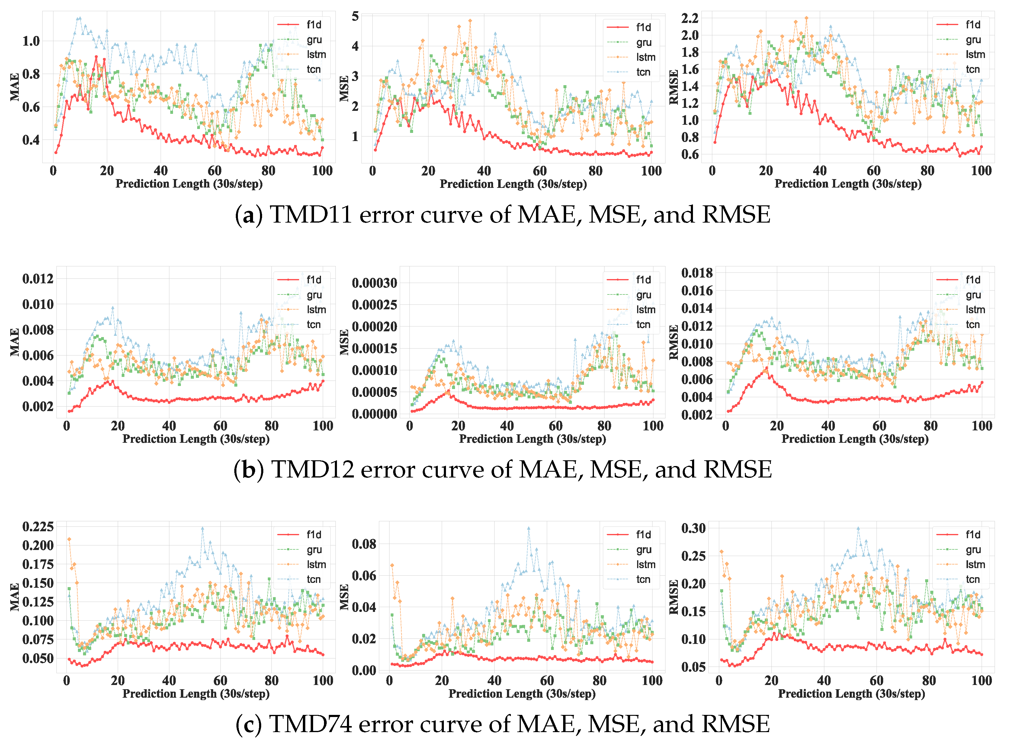
To further assess model performance under varying prediction horizons, we plotted the MAE, MSE, and RMSE curves across forecasting lengths ranging from 1 to 100 steps for three representative telemetry features: TMD11, TMD12, and TMD74. As shown in Figure 6 each curve illustrates the quantitative evolution of prediction error as the horizon increases, providing a more explicit trajectory of accuracy degradation across different models.
Across all three datasets, the proposed F1D model consistently achieves superior performance under all metrics. Its error curves remain substantially lower than those of GRU, LSTM, and TCN, particularly in long-horizon forecasting. Notably, F1D maintains a stable error trajectory with minimal fluctuation and negligible accumulation as the prediction length increases. This observation is consistent with the heatmap results, where F1D exhibited more dispersed and lower-magnitude error distributions without strong diagonal accumulation.
In contrast, the GRU and LSTM baselines display pronounced error growth as the horizon extends, often with oscillatory patterns and peak values at specific steps, highlighting their susceptibility to long-term error propagation. The TCN model, while occasionally competitive in short-range settings, demonstrates the largest and most volatile errors for medium-to-long horizons, indicating limited generalization capacity in modeling long temporal dependencies.
Overall, the comparative analysis of error curves provides strong evidence for the effectiveness of the proposed F1D model in time series forecasting. It not only reduces absolute error but also mitigates cumulative degradation over time, thereby outperforming recurrent and convolutional baselines in both accuracy and stability.

3.3.3. Samples Comparative Visualization

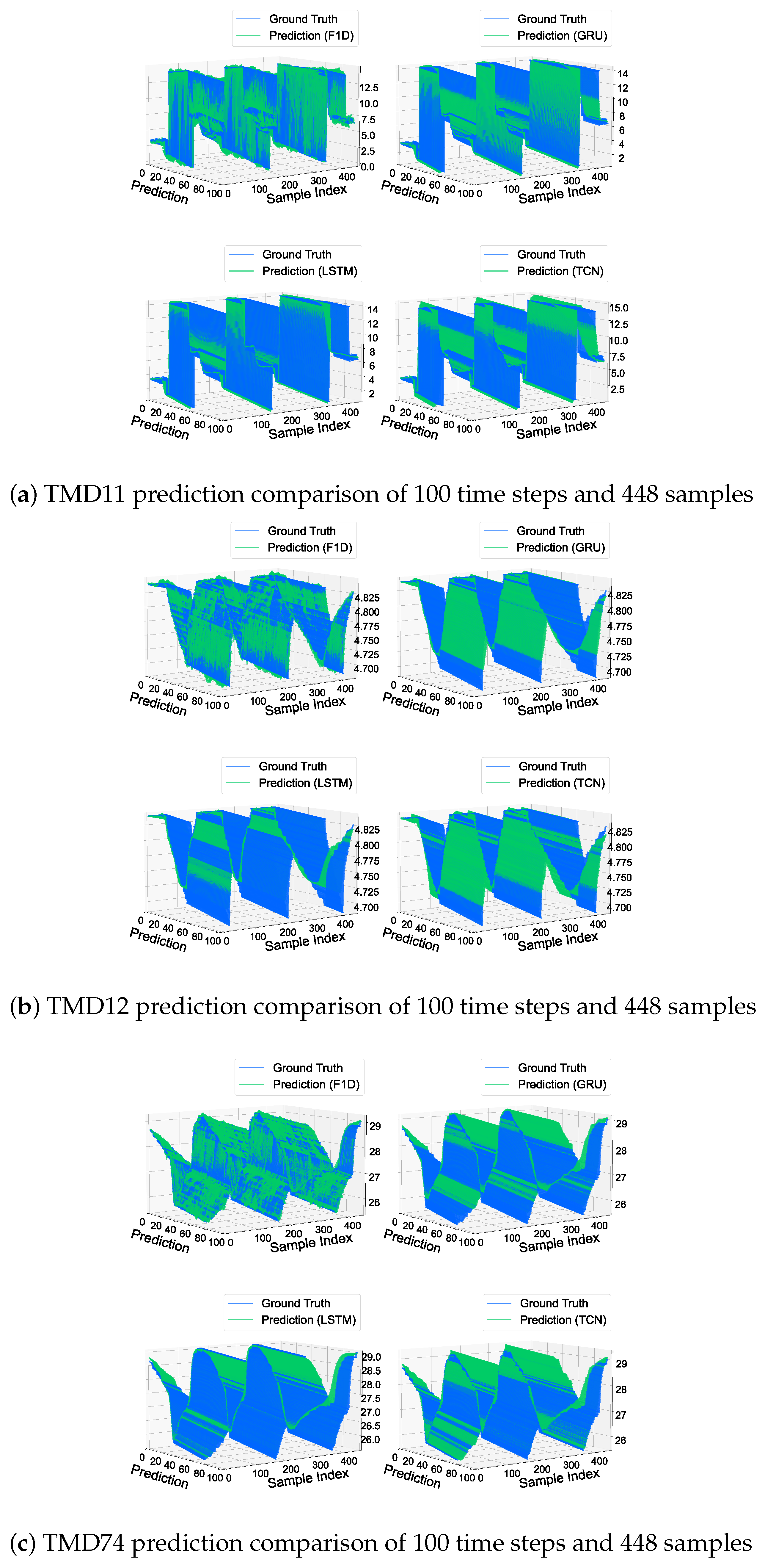
To provide a more intuitive understanding of the models’ forecasting performance, we present 3D comparative visualizations of predicted and ground truth values across 448 test samples for three representative telemetry variables: TMD11, TMD12, and TMD74. As shown in Figure 7, in each subplot, the X-axis represents the prediction step, the Y-axis corresponds to the sample index, and the Z-axis denotes the telemetry value. Ground truth trajectories are depicted as green curves, while the predicted trajectories are plotted in blue.
The proposed F1D model consistently exhibits superior predictive accuracy across all three variables. Its predicted curves are almost indistinguishable from the ground truth, particularly for TMD11 and TMD12, where prediction errors are negligible. Even for the more volatile and challenging TMD74 dataset, F1D demonstrates robust trend-tracking capability and maintains low forecasting errors over extended horizons.
In contrast, GRU and LSTM models produce noticeably larger deviations from the ground truth, especially at longer prediction steps and near the sequence boundaries. Their predicted curves exhibit visible gaps and oscillations, reflecting cumulative error propagation. The TCN model performs the worst overall, with substantial divergence from the ground truth and the presence of high-frequency noise, failing to capture the intrinsic temporal dynamics.

3.3.4. Mean Trajectory Analysis

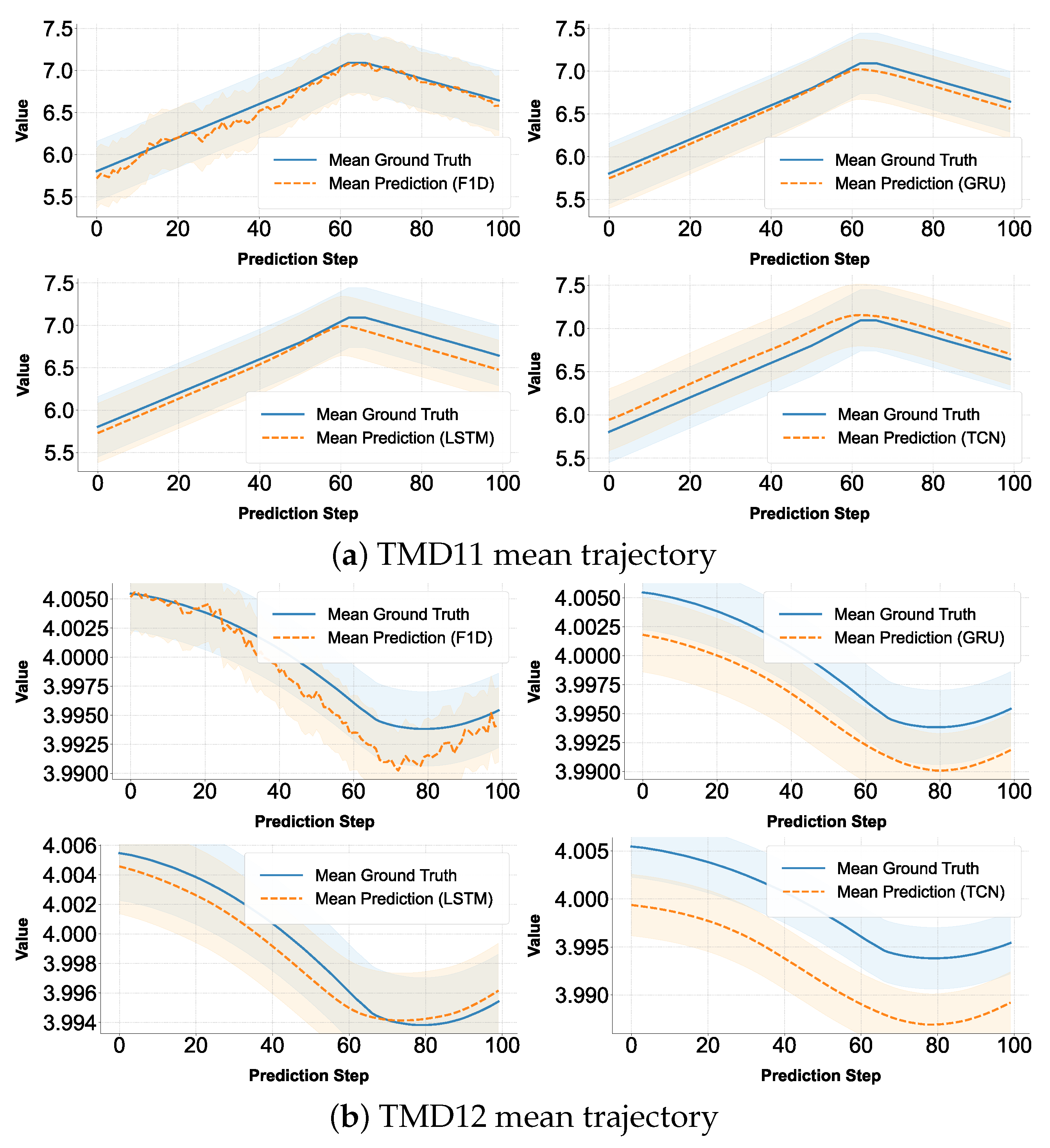
To evaluate each model’s ability to capture global temporal trends, we analyze the mean predicted trajectories against the mean ground truth trajectories across 448 test samples over 100 prediction steps. As shown in Figure 8, in the visualizations, average ground truth values are shown as blue solid lines, while average predicted values are represented as red dashed lines. This perspective emphasizes how well each model approximates the overall structural dynamics of the sequence beyond individual sample accuracy.
Across all three datasets, the proposed F1D model achieves the highest fidelity in following the true mean trajectory. On the challenging TMD11 dataset, which exhibits sharp “V-shaped” variations, F1D maintains the closest correspondence, with only minor deviations near turning points. For TMD12, characterized by a concave “U-shaped” pattern, F1D accurately captures both the trough and the flanking slopes, consistently outperforming all baselines. On TMD74, F1D demonstrates nearly perfect alignment with the ground truth across ascending, plateau, and descending phases.
In contrast, GRU and LSTM tend to over-smooth the mean trajectory and display systematic deviations at inflection points, particularly on TMD12 and TMD74. The TCN model performs the most weakly overall, with predicted trajectories diverging substantially from the actual means across the entire forecasting horizon.

3.3.5. Error Heatmap Analysis

To further assess model performance across the forecasting horizon, we visualize absolute prediction errors for 448 test samples over 100 forecast steps using heatmaps as shown in Figure 9. The GRU, LSTM, and TCN models exhibit a pronounced diagonal pattern, where errors gradually accumulate with longer prediction horizons. Their maximum absolute errors fall within the range of 0.8 to 1.0, reflecting substantial degradation in long-term accuracy.
In contrast, the proposed F1D model demonstrates a markedly different error distribution. Its errors appear more localized and scattered, without the diagonal accumulation trend observed in the baselines. Moreover, its maximum error remains consistently below 0.4, indicating enhanced stability and robustness. These results suggest that F1D not only achieves lower overall prediction errors but also effectively mitigates error drift in long-horizon forecasting, likely owing to its superior ability to capture temporal dependencies.

3.4. Ablation Study

3.4.1. Quantitative Evaluation of Forecasting Performance

To investigate the individual contributions of different architectural components in the proposed model, we construct four ablated variants in addition to a baseline Transformer. These variants are defined as follows:
  • F1D (Full Model): The complete architecture, which incorporates a 1D Fast Fourier Transform (FFT) for temporal frequency decomposition, followed by a Dual-Path Mixer that integrates both time-domain and frequency-domain processing streams. It also includes dynamic positional encoding for adaptive representation of temporal positions.
  • F1: A variant that retains only the 1D FFT-based frequency encoder while removing the dual-path design. This isolates the effect of 1D frequency transformation alone.
  • F2D: A version that replaces the 1D FFT with a 2D FFT encoder, capturing joint time–frequency correlations across both temporal and feature dimensions. The dual-path mixer is retained.
  • F2: A variant that applies only the 2D FFT module without dual-path modeling or positional encoding, aiming to evaluate the standalone effectiveness of global spectral representations.
  • Transformer: The standard Transformer encoder with self-attention and fixed sinusoidal positional encoding, but without any frequency-domain modeling. This serves as the baseline.
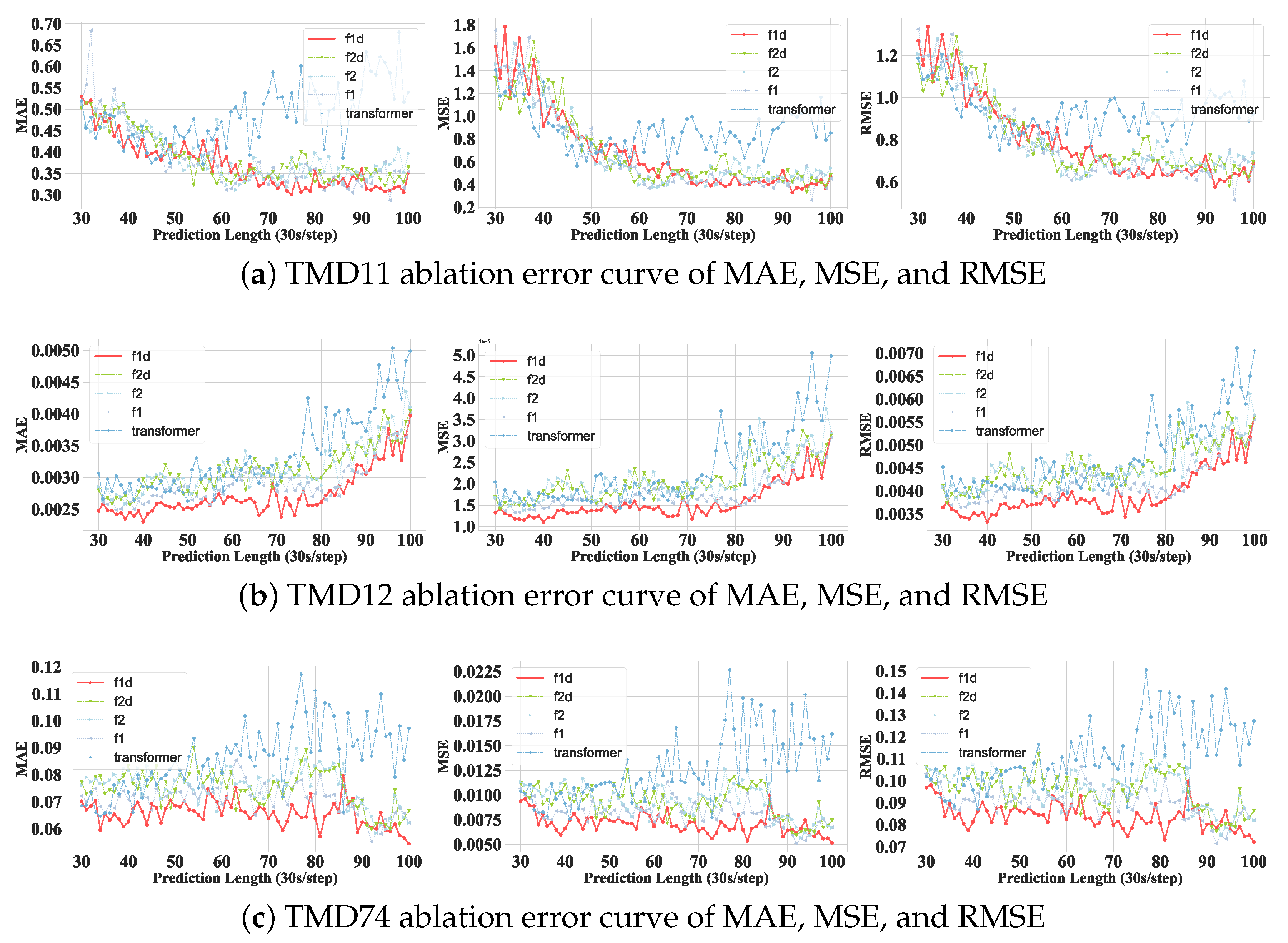
As shown in Table 7, Table 8 and Table 9, F1D consistently achieves the lowest MSE and MAE across nearly all prediction lengths and datasets (TMD11, TMD12, and TMD74). Several key insights can be drawn from these comparisons: On TMD11, F1D demonstrates a clear advantage over all ablations, particularly in long-term forecasting (60–100 steps). For example, at step 100, F1D achieves an MSE of 0.4706, outperforming F1 (0.4536), F2D (0.4848), and Transformer (0.8516), confirming its superior ability to capture long-range dependencies and structural transitions. On TMD12, which exhibits low-magnitude and smooth fluctuations, all models achieve small errors. Nevertheless, F1D still performs marginally better in most cases, validating its robustness on low-variance signals. On TMD74, characterized by irregular and non-stationary telemetry dynamics, F1D consistently outperforms the baselines in both short- and long-horizon settings. Notably, from step 30 onward, F1D maintains consistently lower MAE and MSE. For instance, at step 100, F1D yields an MAE of 0.0545 compared to 0.0623 (F1), 0.0668 (F2D), and 0.0973 (Transformer).
Overall, these results highlight that each component—frequency-aware representation and dual-path modeling—are critical to enhancing forecasting performance. The full model (F1D), benefiting from their joint effect, achieves the most accurate and stable predictions, thereby confirming the effectiveness of the proposed architectural design.

3.4.2. Error Curve Analysis

To further assess model performance under varying prediction horizons, we plotted the MAE, MSE, and RMSE curves across forecasting lengths ranging from 1 to 100 steps for three representative telemetry features: TMD11, TMD12, and TMD74. As shown in Figure 10 each curve illustrates the quantitative evolution of prediction error as the horizon increases, providing a more explicit trajectory of accuracy degradation across different models.
On the TMD11 dataset, which exhibits both smooth trends and sharp fluctuations, the proposed F1D model demonstrates strong overall performance with relatively low and stable errors, particularly in the long-term prediction range (beyond 60 steps). During the earlier stages (30–50 steps), however, certain variants such as F2 and F2D occasionally outperform F1D in terms of MAE, indicating that although F1D is not consistently superior at every step, it maintains a favorable overall trend and robustness across varying horizons. Notably, the error curves of F1D and F2D are highly similar, frequently alternating in lead. This observation highlights the importance of the Dual-Path Mixer, which is retained in both models and appears to be a key driver of performance. In contrast, the simplified variants—F1 (1D FFT only) and F2 (2D FFT only)—exhibit noticeably higher errors and greater volatility, particularly over the medium-to-long term, reflecting performance degradation due to the removal of critical architectural components. The standard Transformer performs the worst across all three metrics, with large fluctuations and the highest overall errors, further demonstrating its limitations in modeling complex, high-variance telemetry signals.
On the TMD12 dataset, which features smoother and lower-amplitude fluctuations, the F1D model again exhibits the best overall performance. Its error curves remain consistently low and flat across the entire prediction range. Although the differences between models are relatively small due to the simplicity of the signal, F1D and F2D clearly outperform the other variants. This consistency suggests that F1D is not only effective on complex signals but also generalizes well to simpler, low-variance settings. F2D’s performance closely follows F1D, reaffirming the strength of the Dual-Path Mixer. The simplified variants F1 and F2 show a moderate increase in both MAE and MSE, particularly in mid-to-long-term horizons. Meanwhile, the standard Transformer once again yields the highest errors and the greatest instability, underscoring the advantage of incorporating frequency-domain modeling even when the signal variance is low.
On the TMD74 dataset, which contains more irregular and delayed patterns, the advantage of F1D becomes more pronounced in the later prediction steps (60–100). Its error curves remain the lowest across most horizons, indicating its strong capacity to capture long-term dependencies and handle signal irregularities. Interestingly, F2D performs nearly on par with F1D throughout, with both models significantly outperforming the rest. This suggests that the combination of 2D FFT and the Dual-Path Mixer is already highly effective in capturing the complex dynamics of TMD74. Simplified models such as F2 and F1 experience a clear drop in performance, with higher and more fluctuating error curves. The Transformer again ranks last in all metrics, struggling to track the temporal complexity of the signal. These results further validate the value of frequency-aware modeling and hybrid time–frequency representations in handling diverse telemetry characteristics.
While the F2D variant exhibits competitive performance in some cases, it is not the most consistent alternative to FFT1D-Dual. As summarized in Table 10, FFT1D-Dual achieves the highest number of best results across all prediction horizons and datasets, followed by the 1D FFT variant (F1). This suggests that applying the Fourier transform solely along the temporal dimension provides a more natural inductive bias for capturing long-range periodicity and maintaining temporal coherence. In contrast, the 2D FFT jointly transforms temporal and feature dimensions, which blurs their semantic distinction and weakens the model’s ability to represent pure temporal dependencies. Therefore, FFT1D-Dual was selected as the main architecture due to its superior consistency, stronger temporal interpretability, and more principled design for time series forecasting.

4. Discussion

The proposed FFT1D-Dual model tackles a key challenge in satellite telemetry forecasting: jointly capturing global periodic structures and local irregular dynamics in long, high-dimensional sequences. By integrating frequency- and time-domain representations through a channel-adaptive Dual-Path Mixer, FFT1D-Dual achieves higher forecasting accuracy with improved efficiency. Replacing the encoder’s self-attention with this mixer substantially enhances long-horizon stability, showing that attention is not always essential when spectral and convolutional features are fused effectively.
Compared with GRU, LSTM, and TCN, which suffer from error drift in long-term prediction, FFT1D-Dual produces more stable error trajectories and lower maximum errors across variables. Gains are evident on both high-variance (TMD11) and low-amplitude (TMD12) signals, confirming its robustness. Ablation studies further indicate the following: (i) frequency-domain modeling alone improves over Transformers but is less robust; and (ii) the Dual-Path Mixer is crucial for handling heterogeneous dynamics.
Limitations include the assumption of regularly sampled data and the limited interpretability of the gating mechanism. Future work will extend to irregular, multivariate, and event-driven telemetry, while exploring physical interpretations of gating dynamics.
In conclusion, FFT1D-Dual offers a scalable and interpretable solution for long-term satellite forecasting, balancing accuracy and efficiency, and showing strong potential for real-time health monitoring and predictive control.

Author Contributions

Conceptualization and methodology, Z.C. (Zhuqing Chen); validation, Z.Y. and Z.C. (Zhimin Chen); formal analysis and supervision, J.Y.; data preparation, Z.Y. and Y.W.; visualization, L.Z.; writing—original draft, Z.C. (Zhuqing Chen); writing—review and editing, J.Y., Q.J., and Z.C. (Zhimin Chen). All authors have read and agreed to the published version of the manuscript.

Funding

This research was funded by XTT-1 Ground Test System under grant number E16D05A31S.

Data Availability Statement

The data and code supporting the findings of this study will be made publicly available on GitHub after acceptance: https://github.com/iluciddream/F1D-open-source.

Conflicts of Interest

The authors declare no conflicts of interest.

References

  1. Wan, P.; Zhan, Y.; Jiang, W. Study on the Satellite Telemetry Data Classification Based on Self-Learning. IEEE Access 2019, 8, 2656–2669. [Google Scholar] [CrossRef]
  2. Lai, Y.; Zhu, Y.; Li, L.; Lan, Q.; Zuo, Y. STGLR: A Spacecraft Anomaly Detection Method Based on Spatio-Temporal Graph Learning. Sensors 2025, 25, 310. [Google Scholar] [CrossRef]
  3. Napoli, C.; De Magistris, G.; Ciancarelli, C.; Corallo, F.; Russo, F.; Nardi, D. Exploiting Wavelet Recurrent Neural Networks for Satellite Telemetry Data Modeling, Prediction and Control. Expert Syst. Appl. 2022, 206, 117831. [Google Scholar] [CrossRef]
  4. Fejjari, A.; Delavault, A.; Camilleri, R.; Valentino, G. A Review of Anomaly Detection in Spacecraft Telemetry Data. Appl. Sci. 2025, 15, 5653. [Google Scholar] [CrossRef]
  5. Neto, J.C.A.; Farias, C.M.; Araujo, L.S.; Filho, L.A.D.L. Time Series Forecasting for Multidimensional Telemetry Data Using GAN and BiLSTM in a Digital Twin. arXiv 2025, arXiv:2501.08464. [Google Scholar] [CrossRef]
  6. Lin, C.; Junyu, C. Using Long Short-Term Memory Neural Network for Satellite Orbit Prediction Based on Two-Line Element Data. IEEE Trans. Aerosp. Electron. Syst. 2025, 2025, 1–10. [Google Scholar] [CrossRef]
  7. Guo, Y.; Li, B.; Shi, X.; Zhao, Z.; Sun, J.; Wang, J. Enhancing Medium-Orbit Satellite Orbit Prediction: Application and Experimental Validation of the BiLSTM-TS Model. Electronics 2025, 14, 1734. [Google Scholar] [CrossRef]
  8. Kricheff, S.; Maxwell, E.; Plaks, C.; Simon, M. An Explainable Machine Learning Approach for Anomaly Detection in Satellite Telemetry Data. In Proceedings of the 2024 IEEE Aerospace Conference, Big Sky, MT, USA, 2–9 March 2024; pp. 1–14. [Google Scholar] [CrossRef]
  9. Xu, Y.; Yao, W.; Zheng, X.; Chen, J. A Hybrid Monte Carlo Quantile EMD-LSTM Method for Satellite In-Orbit Temperature Prediction and Data Uncertainty Quantification. Expert Syst. Appl. 2024, 255, 124875. [Google Scholar] [CrossRef]
  10. Knap, V.; Bonvang, G.A.P.; Fagerlund, F.R.; Krøyer, S.; Nguyen, K.; Thorsager, M.; Tan, Z.-H. Extending Battery Life in CubeSats by Charging Current Control Utilizing a Long Short-Term Memory Network for Solar Power Predictions. J. Power Sources 2024, 618, 235164. [Google Scholar] [CrossRef]
  11. Peng, Y.; Jia, S.; Xie, L.; Shang, J. Accurate Satellite Operation Predictions Using Attention-BiLSTM Model with Telemetry Correlation. Aerospace 2024, 11, 398. [Google Scholar] [CrossRef]
  12. Xu, Z.; Cheng, Z.; Guo, B. A Multivariate Anomaly Detector for Satellite Telemetry Data Using Temporal Attention-Based LSTM Autoencoder. IEEE Trans. Instrum. Meas. 2023, 72, 3296125. [Google Scholar] [CrossRef]
  13. Wang, Y.; Gong, J.; Zhang, J.; Han, X. A Deep Learning Anomaly Detection Framework for Satellite Telemetry with Fake Anomalies. Int. J. Aerosp. Eng. 2022, 2022, 1–9. [Google Scholar] [CrossRef]
  14. Zeng, Z.; Jin, G.; Xu, C.; Chen, S.; Zhelong, Z.; Zhang, L. Satellite Telemetry Data Anomaly Detection Using Causal Network and Feature-Attention-Based LSTM. IEEE Trans. Instrum. Meas. 2022, 71, 1–21. [Google Scholar] [CrossRef]
  15. Yang, L.; Ma, Y.; Zeng, F.; Peng, X.; Liu, D. Improved Deep Learning Based Telemetry Data Anomaly Detection to Enhance Spacecraft Operation Reliability. Microelectron. Reliab. 2021, 126, 114311. [Google Scholar] [CrossRef]
  16. Tao, L.; Zhang, T.; Peng, D.; Hao, J.; Jia, Y.; Lu, C.; Ding, Y.; Ma, L. Long-Term Degradation Prediction and Assessment with Heteroscedasticity Telemetry Data Based on GRU-GARCH and MD Hybrid Method: An Application for Satellite. Aerosp. Sci. Technol. 2021, 115, 106826. [Google Scholar] [CrossRef]
  17. Gallon, R.; Schiemenz, F.; Menicucci, A.; Gill, E. Convolutional Neural Network Design and Evaluation for Real-Time Multivariate Time Series Fault Detection in Spacecraft Attitude Sensors. Adv. Space Res. 2025, 76, 2960–2976. [Google Scholar] [CrossRef]
  18. Tang, H.; Cheng, Y.; Lu, N.; Han, X. Anomaly Detection in Satellite Attitude Control System Based on GAT-TCN. In Proceedings of the 2024 Global Reliability and Prognostics and Health Management Conference (PHM-Beijing), Beijing, China, 17–20 June 2024; pp. 1–8. [Google Scholar] [CrossRef]
  19. Zeng, Z.; Lei, J.; Jin, G.; Xu, C.; Zhang, L. Detecting Anomalies in Satellite Telemetry Data Based on Causal Multivariate Temporal Convolutional Network. In Proceedings of the 2022 IEEE 5th International Conference on Big Data and Artificial Intelligence (BDAI), Fuzhou, China, 17–19 December 2022; pp. 63–74. [Google Scholar] [CrossRef]
  20. Noh, S.-H. Analysis of Gradient Vanishing of RNNs and Performance Comparison. Information 2021, 12, 442. [Google Scholar] [CrossRef]
  21. Tu, T. Bridging Short- and Long-Term Dependencies: A CNN-Transformer Hybrid for Financial Time Series Forecasting. arXiv 2025, arXiv:2504.19309. [Google Scholar] [CrossRef]
  22. Vaswani, A.; Shazeer, N.; Parmar, N.; Uszkoreit, J.; Jones, L.; Gomez, A.N.; Kaiser, L.; Polosukhin, I. Attention Is All You Need. arXiv 2017, arXiv:1706.03762. [Google Scholar] [CrossRef]
  23. Zhou, H.; Zhang, S.; Peng, J.; Zhang, S.; Li, J.; Xiong, H.; Zhang, W. Informer: Beyond Efficient Transformer for Long Sequence Time-Series Forecasting. In Proceedings of the Thirty-Fifth AAAI Conference on Artificial Intelligence (AAAI 2021), Virtual, 2–9 February 2021; pp. 11106–11115. [Google Scholar] [CrossRef]
  24. Zhou, H.; Li, J.; Zhang, S.; Zhang, S.; Yan, M.; Xiong, H. Expanding the Prediction Capacity in Long Sequence Time-Series Forecasting. Artif. Intell. 2023, 318, 103886. [Google Scholar] [CrossRef]
  25. Su, L.; Zuo, X.; Li, R.; Wang, X.; Zhao, H.; Huang, B. A Systematic Review for Transformer-Based Long-Term Series Forecasting. Artif. Intell. Rev. 2025, 58, 80. [Google Scholar] [CrossRef]
  26. Qiao, Y.; Wang, T.; Lü, J.; Liu, K. TEMPO: Time-Evolving Multi-Period Observational Anomaly Detection Method for Space Probes. Chin. J. Aeronaut. 2025, 38, 103426. [Google Scholar] [CrossRef]
  27. Song, B.; Guo, B.; Hu, W.; Zhang, Z.; Zhang, N.; Bao, J.; Wang, J.; Xin, J. Transformer-Based Time-Series Forecasting for Telemetry Data in an Environmental Control and Life Support System of Spacecraft. Electronics 2025, 14, 459. [Google Scholar] [CrossRef]
  28. Park, K.-S.; Yun, S.-T. A Data-Driven Battery Degradation Estimation Method for Low-Earth-Orbit (LEO) Satellites. Appl. Sci. 2025, 15, 2182. [Google Scholar] [CrossRef]
  29. Gao, Y.; Qiu, S.; Liu, M.; Zhang, L.; Cao, X. Fault Warning of Satellite Momentum Wheels with a Lightweight Transformer Improved by FastDTW. IEEE/CAA J. Autom. Sin. 2025, 12, 539–549. [Google Scholar] [CrossRef]
  30. Zhao, H.; Qiu, S.; Yang, J.; Guo, J.; Liu, M.; Cao, X. Satellite Early Anomaly Detection Using an Advanced Transformer Architecture for Non-Stationary Telemetry Data. IEEE Trans. Consum. Electron. 2024, 70, 4213–4225. [Google Scholar] [CrossRef]
  31. Lan, Q.; Zhu, Y.; Lin, B.; Zuo, Y.; Lai, Y. Fault Prediction for Rotating Mechanism of Satellite Based on SSA and Improved Informer. Appl. Sci. 2024, 14, 9412. [Google Scholar] [CrossRef]
  32. Lee-Thorp, J.; Ainslie, J.; Eckstein, I.; Ontanon, S. FNet: Mixing Tokens with Fourier Transforms. arXiv 2022, arXiv:2105.03824. [Google Scholar] [CrossRef]
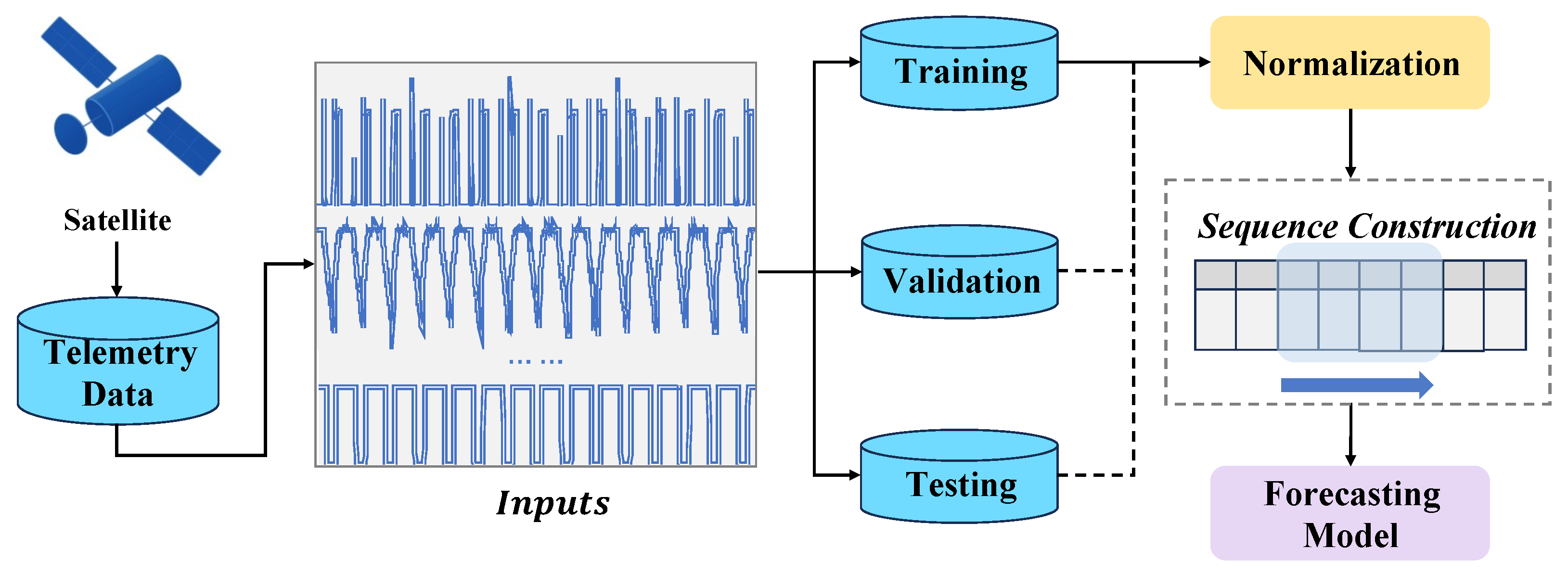
Figure 1. End-to-End time series model framework for satellite telemetry data forecasting.
Applsci 15 11585 g001
Figure 2. FFT1D-Dual prediction model architecture.
Applsci 15 11585 g002
Figure 3. Architecture of the Dual-Path Mixer Module.
Applsci 15 11585 g003
Figure 4. Architecture of the Fourier Mixer Module.
Applsci 15 11585 g004
Figure 5. Predictions over 100 time steps for TMD11, TMD12, and TMD74 (ac).
Applsci 15 11585 g005
Figure 6. Error curves of TMD11, TMD12, and TMD74 (ac).
Applsci 15 11585 g006
Figure 7. Prediction 3D visualizations of 100 time steps and 448 samples for TMD11, TMD12, and TMD74 (ac).
Applsci 15 11585 g007
Figure 8. Mean trajectory of 100 time steps over all samples for TMD11, TMD12, and TMD74 (ac).
Applsci 15 11585 g008aApplsci 15 11585 g008b
Figure 9. Error heatmap of 100 time steps over all samples for TMD11, TMD12, and TMD74 (ac).
Applsci 15 11585 g009aApplsci 15 11585 g009b
Figure 10. Ablation error curves of TMD11, TMD12, and TMD74 (ac).
Applsci 15 11585 g010
Table 1. Representative summary of dataset parameters.
ParameterTypeUnitDescription
TMD01IntegerCountsTotal count of telemetry request commands (CAN bus)
TMD07FloatVVoltage of the 42 V main power bus
TMD08FloatVVoltage of the 30 V power bus
TMD09FloatVTotal voltage of the battery pack
TMD11FloatVVoltage of BEA (specific module/component)
TMD12FloatVVoltage of the 1st lithium-ion cell in the pack
TMD21FloatVVoltage measured across the 1st shunt
TMD37FloatVOutput of charge voltage setpoint (charging module)
TMD52FloatATotal load current of the 42 V bus
TMD54FloatABattery charging current
TMD55FloatABattery discharging current
TMD56FloatAOutput current of the S4R1 solar array
TMD59FloatAOutput current of BDR (module 1)
TMD69Float°CInternal temperature of the power controller
TMD74Float°CTemperature from the 5th battery-pack sensor
Table 2. Model configuration and training settings.
CategoryConfiguration
Model Architecture
Encoder input dimension69
Decoder input dimension69
Output dimension1
Model dimension ( d m o d e l )512
Feedforward dimension ( d f f )2048
Encoder layers2
Decoder layers1
Attention heads4
Attention typeFull (scaled dot-product)
Dropout rate0.03
Activation functionGELU
DistillationDisabled
Dynamic positional encodingEnabled
Training Hyperparameters
Batch size32
Learning rate 3 × 10 4
Loss functionMAE
Learning rate adjustmentType-1 scheduler
Training epochs50
Patience (early stopping)3
PrecisionFP32 (AMP disabled)
Optimizer workers0 (single-threaded dataloader)
Prediction Settings
Prediction length ( L p r e d )1–100
Label length ( L l a b e l ) = L p r e d
Input length ( L i n p u t ) = 2 × L p r e d
Table 3. Experimental hardware and software environment.
CategoryConfiguration
FrameworkPyTorch 2.1.0
LanguagePython 3.8.20
GPUNVIDIA GeForce RTX 4060 Laptop GPU, 8 GB VRAM
CUDA/DriverCUDA 12.6/NVIDIA Driver 560.94
CPUIntel Core i7-13650HX, 14 Cores/20 Threads, 2.6 GHz
Memory24 GB DDR5 4800 MHz
Storage512 GB SSD
OSMicrosoft Windows 11
Table 4. Forecasting results on TMD11 with different prediction horizons.
HorizonF1D (Proposed)GRULSTMTCN
MSEMAEMSEMAEMSEMAEMSEMAE
10.55890.35701.10890.45681.26020.46140.70100.4686
102.26190.72981.36300.67372.25000.87613.02381.1381
202.06150.72012.73410.80232.00220.64162.88711.0630
301.61410.52901.75560.57983.72190.66922.95990.9361
400.91510.43583.32840.68102.79730.65023.67410.9034
500.66740.38731.64620.67832.96230.60833.07000.8588
600.57880.36860.62470.43710.81590.36111.42890.6582
700.51050.34761.97810.64611.73360.62181.98260.7837
800.48820.35832.26660.94221.03320.57411.86600.9531
900.52280.36051.85980.77212.78930.73582.18791.0832
1000.47060.35200.68600.39941.47600.52452.16600.9379
Note: Bold values indicate the best performance (lowest MSE and MAE) for each prediction horizon.
Table 5. Forecasting results on TMD12 with different prediction horizons.
HorizonF1D (Proposed)GRULSTMTCN
MSEMAEMSEMAEMSEMAEMSEMAE
14.3 × 10 6 0.00141.6 × 10 5 0.00241.3  × 10 5 0.00231.7 × 10 6 0.0029
102.6  × 10 5 0.00300.00010.00679.7 × 10 5 0.00600.00010.0076
202.9  × 10 5 0.00346.8 × 10 5 0.00530.00010.00680.00010.0087
301.3  × 10 5 0.00256.2 × 10 5 0.00486.1 × 10 5 0.00547.1 × 10 5 0.0056
401.1  × 10 5 0.00236.9 × 10 5 0.00535.5 × 10 5 0.00495.6 × 10 5 0.0050
501.4  × 10 5 0.00254.8 × 10 5 0.00475.1 × 10 5 0.00506.3 × 10 5 0.0054
601.4  × 10 5 0.00274.1 × 10 5 0.00474.4 × 10 5 0.00476.4 × 10 5 0.0062
701.5  × 10 5 0.00277.0 × 10 5 0.00575.7 × 10 5 0.00488.0 × 10 5 0.0067
801.5  × 10 5 0.00260.00010.00690.00010.00710.00020.0084
902.0  × 10 5 0.00310.00010.00720.00010.00660.00030.0113
1003.2  × 10 5 0.00405.2 × 10 5 0.00450.00010.00590.00030.0114
Note: Bold values indicate the best performance (lowest MSE and MAE) for each prediction horizon.
Table 6. Forecasting results on TMD74 with different prediction horizons.
HorizonF1D (Proposed)GRULSTMTCN
MSEMAEMSEMAEMSEMAEMSEMAE
10.00350.04730.00750.06660.00580.05800.00700.0638
100.00440.04880.01280.07250.01140.07480.01010.0711
200.00970.06950.01410.08020.01650.08970.02330.1055
300.00940.07030.01160.07370.02550.09190.02890.1151
400.00670.06260.02030.09440.02730.10960.03790.1364
500.00750.06860.02760.11470.04110.13310.06100.1744
600.00680.06490.02470.11370.03440.12700.05180.1629
700.00640.06380.02080.10550.02010.10010.03190.1270
800.00650.06380.02660.12160.02230.10040.02600.1156
900.00640.06240.02960.12220.01610.09410.02470.1222
1000.00520.05450.02400.12040.02270.10560.03120.1290
Note: Bold values indicate the best performance (lowest MSE and MAE) for each prediction horizon.
Table 7. Forecasting results on TMD11 with different prediction horizons.
HorizonF1D (Proposed)F1F2DF2Transformer
MSEMAEMSEMAEMSEMAEMSEMAEMSEMAE
10.55890.35700.54150.32810.54970.33460.53460.31220.55740.3398
102.26190.72982.19740.63481.74900.73861.81490.67882.03000.6027
202.06150.72012.11380.61162.09540.64031.94070.66422.00330.7147
301.61410.52901.75540.51721.33710.50271.45670.51251.40700.5198
400.91510.43581.25880.45031.22510.47951.18740.46621.30140.4345
500.66740.38730.89310.39820.78970.39180.66900.42070.76780.4587
600.57880.36860.48620.32950.47120.34950.39800.34710.94990.4716
700.51050.34760.41360.32360.52450.34100.50790.34980.97390.5393
800.48820.35830.48290.36110.49010.33020.63040.39840.82720.5436
900.52280.36050.42150.31970.43020.33400.46240.34520.95190.5456
1000.47060.35200.45360.35510.48480.36480.54510.39680.85160.5395
Note: Bold values indicate the best performance (lowest MSE and MAE) for each prediction horizon.
Table 8. Forecasting results on TMD12 with different prediction horizons.
HorizonF1D (Proposed)F1F2DF2Transformer
MSEMAEMSEMAEMSEMAEMSEMAEMSEMAE
14.3 × 10 6 0.00146.1 × 10 6 0.00175.5 × 10 6 0.00165.3 × 10 6 0.00155.3 × 10 6 0.0015
102.6 × 10 5 0.00302.9 × 10 5 0.00332.7 × 10 5 0.00343.1 × 10 5 0.00372.7 × 10 5 0.0031
202.9 × 10 5 0.00342.9 × 10 5 0.00343.4 × 10 5 0.00382.4 × 10 5 0.00342.3 × 10 5 0.0032
301.3 × 10 5 0.00251.6 × 10 5 0.00281.6 × 10 5 0.00281.7 × 10 5 0.00292.0 × 10 5 0.0031
401.1 × 10 5 0.00231.4 × 10 5 0.00251.8 × 10 5 0.00291.6 × 10 5 0.00271.8 × 10 5 0.0029
501.4 × 10 5 0.00251.6 × 10 5 0.00281.6 × 10 5 0.00271.7 × 10 5 0.00281.6 × 10 5 0.0026
601.4 × 10 5 0.00271.7 × 10 5 0.00291.9 × 10 5 0.00302.0 × 10 5 0.00301.8 × 10 5 0.0030
701.5 × 10 5 0.00271.5 × 10 5 0.00271.9 × 10 5 0.00322.0 × 10 5 0.00331.7 × 10 5 0.0029
801.5 × 10 5 0.00261.6 × 10 5 0.00271.9 × 10 5 0.00301.9 × 10 5 0.00292.4 × 10 5 0.0034
902.0 × 10 5 0.00312.0 × 10 5 0.00302.3 × 10 5 0.00332.4 × 10 5 0.00342.7 × 10 5 0.0037
1003.2 × 10 5 0.00403.1 × 10 5 0.00403.1 × 10 5 0.00403.2 × 10 5 0.00414.9 × 10 5 0.0050
Note: Bold values indicate the best performance (lowest MSE and MAE) for each prediction horizon.
Table 9. Forecasting results on TMD74 with different prediction horizons.
HorizonF1D (Proposed)F1F2DF2Transformer
MSEMAEMSEMAEMSEMAEMSEMAEMSEMAE
10.00350.04730.00270.04100.00320.04500.00270.04250.00250.0398
100.00440.04880.00400.04650.00410.04710.00500.05290.00530.0527
200.00970.06950.00930.06540.00950.06740.00890.07150.01690.0802
300.00940.07030.01070.07230.01130.07740.01130.07620.01040.0687
400.00670.06260.00820.07080.01110.08330.01160.08180.00920.0436
500.00750.06860.00810.07360.00880.07440.00940.07800.01130.0850
600.00680.06490.00730.06900.01030.08090.00900.07700.01070.0807
700.00640.06380.00880.07330.00910.07210.01010.07780.01160.0872
800.00650.06380.00820.07310.01080.08240.01160.08330.01980.1113
900.00640.06240.00800.07100.00780.07040.00780.06960.01240.0855
1000.00520.05450.00670.06230.00750.06680.00670.06230.01620.0973
Note: Bold values indicate the best performance (lowest MSE and MAE) for each prediction horizon.
Table 10. Model winning counts across all horizons and variables.
ModelCount
F1D (Proposed)37
F120
F2D5
F24
Transformer4
Disclaimer/Publisher’s Note: The statements, opinions and data contained in all publications are solely those of the individual author(s) and contributor(s) and not of MDPI and/or the editor(s). MDPI and/or the editor(s) disclaim responsibility for any injury to people or property resulting from any ideas, methods, instructions or products referred to in the content.