Research on Fault Diagnosis Method for Autonomous Underwater Vehicles Based on Improved LSTM Under Data Missing Conditions

Abstract

Fault diagnosis for Autonomous underwater Vehicle (AUVs) is a key technology for ensuring the safety of AUVs and an important skill for enabling them to autonomously perform tasks underwater for long periods. The effectiveness of current diagnostic methods is affected by the reliability of expert knowledge and the accuracy of model establishment. In addition, some data-driven diagnostic methods lack robustness. Unlike traditional model-based fault diagnosis methods, this paper proposes a fault diagnosis method for AUVs based on the LSTM (Long Short-Term Memory) algorithm. LSTM is good at processing time series data and can learn complex temporal patterns. Therefore, the LSTM model is used to learn the mapping of state data to its corresponding fault types. The underwater environment in which AUVs work is complex and ever-changing, and packet loss may occur during data transmission, resulting in partial loss of online data. To address this issue, this paper fills in missing values during the feature processing stage and then uses a BiLSTM-Attention-MiniLoss algorithm to enhance the robustness of the diagnostic model. Finally, the fault diagnosis accuracy of the original LSTM and the BiLSTM-Attention-MiniLoss was compared based on an open-source dataset under different degrees of data loss. The experimental results showed that the fault diagnosis methods for AUV based on LSTM and the BiLSTM-Attention-MiniLoss could predict the type of fault based on the navigation status data of the AUV, with BiLSTM-Attention-MiniLoss performing better.

1. Introduction

As a core equipment for deep-sea exploration and marine scientific research, autonomous underwater vehicles (AUVs) have experienced rapid development in recent years. To operate autonomously in complex and unknown environments, AUVs must possess fault diagnosis capabilities to monitor and isolate failures that could lead to mission failure. Fault diagnosis involves three key technologies: fault detection, fault isolation, and fault identification. Research on AUV fault diagnosis primarily focuses on actuator faults and sensor faults [1]. Commonly used fault diagnosis methods include rule-based diagnosis, model-based diagnosis, and data-driven diagnosis [2,3,4,5,6].

1.1. Rule-Based Diagnosis

The core idea of rule-based diagnosis is to transform the knowledge mastered by experts into diagnostic rules and implement fault diagnosis based on the diagnostic rules. The process is shown in Figure 1. Ranganathan et al. [7] proposed an intelligent system for AUVs that integrates fault detection and control functions to ensure safety in case of faults. Hamilton K et al. [8] proposed an integrated diagnostic framework for health management of AUVs, combining expert systems with real-time monitoring. Zheng Y et al. [9] designed a diagnostic expert system based on finite state machine (FSM) for fault diagnosis of large autonomous unmanned submarines. Miguelanez et al. [10] proposed a semantic knowledge-based framework that combines expert localization with observation data to enhance the semantic interpretation ability of fault monitoring and improve the situational awareness of AUVs, enabling them to better understand the environment and make decisions. The rule-based diagnostic method has a short execution time, but the knowledge rules overly rely on expert experience and are difficult to handle scenarios where multiple faults occur simultaneously [11,12,13]. However, there are some key problems with AUV fault diagnosis models that are based on rules. However, rule-based AUV diagnostic models face several challenges. Primarily, the multitude of attributes generated by AUV sensors leads to an exponential increase in the total number of rules, resulting in a “combinatorial explosion” problem. Furthermore, during actual AUV operations, observational data may be affected by various interfering factors. The presence of noise in the observed data adversely impacts the accuracy and reliability of this methodology.

1.2. Model-Based Diagnosis

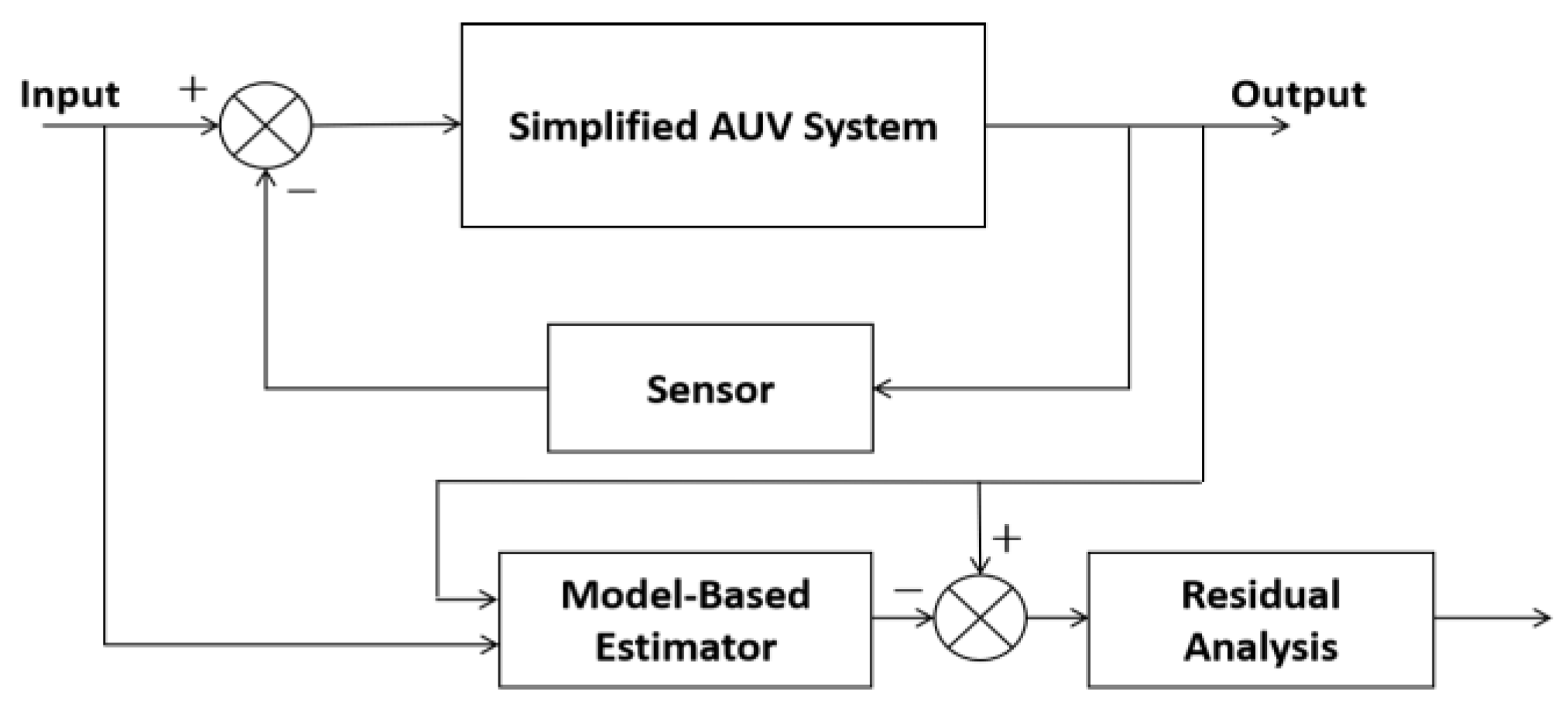
The core idea of model-based diagnostic methods is to reconstruct the system process state to obtain residual sequences for fault diagnosis [14]. Firstly, establish the mathematical model of AUV, and then use observer, parameter estimation or residual generation techniques for fault detection and isolation, the process is shown in Figure 2. Shumsky et al. [15] designed a nonlinear state observer that uses the control input of the AUV and some sensor measurements as inputs to estimate the state of the AUV. Compare the state values estimated by the observer with the actual sensor measurements to generate residual signals. Determine whether a fault has occurred based on the size of the residual value. Chu et al. [16] designed an observer-based fault detection method for the propulsion system of the manned submersible Jiaolong, and improved its model accuracy by combining recursive neural networks. Jiang et al. [17] established motion and thruster fault models for AUVs based on the Strong Tracking Filter (STF) theory. They achieved thruster fault diagnosis by performing online estimation of the AUV’s state variables and thruster fault deviations, followed by residual analysis. The effectiveness of model-based diagnostic methods is limited by model accuracy, and obtaining an accurate model is very difficult. The modeling of nonlinear systems such as AUVs requires extremely complex mathematical and professional knowledge, and there is nonlinear coupling between the six degrees of freedom of AUVs [18]. The complex and varied marine environment in which AUVs operate inevitably results in a lot of interference and noise, which limits the application of model-based fault diagnosis methods in the field of AUV fault diagnosis [19]. Such approaches provide profound insights into the fundamental mechanisms of target systems. However, for complex dynamic systems like AUVs, establishing highly reliable mathematical models proves extremely challenging due to their highly coupled six-degree-of-freedom motion, difficult-to-determine hydrodynamic parameters, and high susceptibility to oceanic current disturbances. These constraints significantly limit related fault diagnosis efforts.

1.3. Data-Driven Diagnosis

Data-driven fault diagnosis method, also known as model-free fault diagnosis or intelligent fault diagnosis [20]. This method constructs a diagnostic model that can automatically connect the data collected from AUV with their health status, as shown in Figure 3:

The data-driven approach is based on machine learning theory, automatically learning its relationship with fault types from collected data. Liu et al. [21] proposed and developed a complete integrated system for fault diagnosis and fault-tolerant control, based on the FCA-CMAC neural network structure, aimed at solving the problem of sudden actuator (such as thruster) failure in unmanned underwater vehicles (UUVs) during critical tasks. Zhang et al. [22] proposed an intelligent fault diagnosis method based on fuzzy weighted support vector domain description, which effectively solves the problem of multi fault diagnosis and provides a solution for imbalanced data. Nascimento et al. [23] took the lead in using a powerful LSTM network to construct a high-precision dynamic behavior model for the soft fault problem of underwater thrusters, and implemented an effective residual generative fault diagnosis strategy based on this model. Jiang et al. [24] used principal component analysis, a multivariate statistical tool, to monitor the health status of actuators by modeling sensor data under normal operating conditions of AUVs. Xia et al. [25] proposed a novel hierarchical attention mechanism framework for deep fusion of multi-source sensor data, thereby achieving more accurate and robust fault diagnosis. A novel hybrid framework for underwater thruster fault detection based on a combination of physical models and generative adversarial networks (GANs) has been proposed.

The data-driven approach does not require building a system model, but it requires a large amount of data to complete the training process, which can make the fault diagnosis system more complex and time-consuming. Moreover, the existing shallow network structure is difficult to mine and extract deeper feature information from fault data, which limits further improvement in accuracy [26,27,28]. However, data-driven approaches have high requirements for data quality. When faced with perturbed data samples from actual operational scenarios of AUVs, they may suffer from data bias, which can impair the accuracy and generalizability of the models [29].

Model-based diagnostic approaches offer benefits such as minimal data requirements and high accuracy. However, their applicability in complex AUV operational scenarios is often limited by challenges, including intricate model construction and sensitivity to initial conditions [30]. To circumvent the difficulties associated with developing accurate physical models, this study employs data-driven methodologies. These approaches demonstrate greater flexibility by automatically identifying and classifying faults through the analysis of and learning from large historical datasets.

Failures in AUVs generally progress incrementally rather than occurring spontaneously, characterized by specific patterns within time-series sensor measurements. The Long Short-Term Memory (LSTM) algorithm is exceptionally suited for this diagnostic task due to its inherent capability to model complex temporal dependencies. Since AUVs are equipped with a diverse array of sensors, traditional diagnostic methods often depend on labor-intensive feature engineering to manually extract and integrate relevant information. In contrast, LSTM serves as an end-to-end model that can autonomously learn discriminative, fault-related features directly from raw or minimally preprocessed multi-sensor data streams, eliminating the need for manual intervention.

Previous research has given little consideration to the problem of missing AUV voyage data and the differential losses caused by diagnostic inaccuracies. Therefore, we propose a BiLSTM model that integrates a temporal-aware feature attention mechanism and a minimum-risk-based loss function to enhance the robustness and accuracy of the diagnostic model.

This paper is organized as follows: Section 1 presents the research background; Section 2 describes the fault diagnosis process for AUVs; Section 3 provides detailed information on the dataset, feature selection methods, and data preprocessing; Section 4 introduces the baseline diagnostic model and its improved versions; Section 5 discusses the experimental procedure and results; and finally, Section 6 concludes the paper.

2. Diagnostic Process

In order to solve the above problems, this paper proposes a deep learning based AUV fault diagnosis model, and the diagnosis process is shown in Figure 4:

The fault diagnosis model is trained offline on historical data, which comprises extensive AUV navigation states and their corresponding fault types. Features that contain fault information are extracted from the dataset to form feature vectors for model training and testing. This training process essentially establishes a mapping from the state data to the fault types, aiming to minimize the discrepancy between the model’s predictions and the actual labels. Once a satisfactory model is obtained, online fault diagnosis can be performed by feeding the current AUV state data into this trained model to predict the fault type in real-time.

3. Data and Features

Learning the mapping from state data to fault types is a typical pattern recognition problem. Therefore, the workflow primarily consists of key steps including data collection, feature extraction, model training, and model testing. In order to improve the quality of feature vectors, it is necessary to preprocess the data. Data preprocessing includes steps such as data standardization and missing value filling, which can improve the training and prediction speed of the model.

3.1. Data Collection

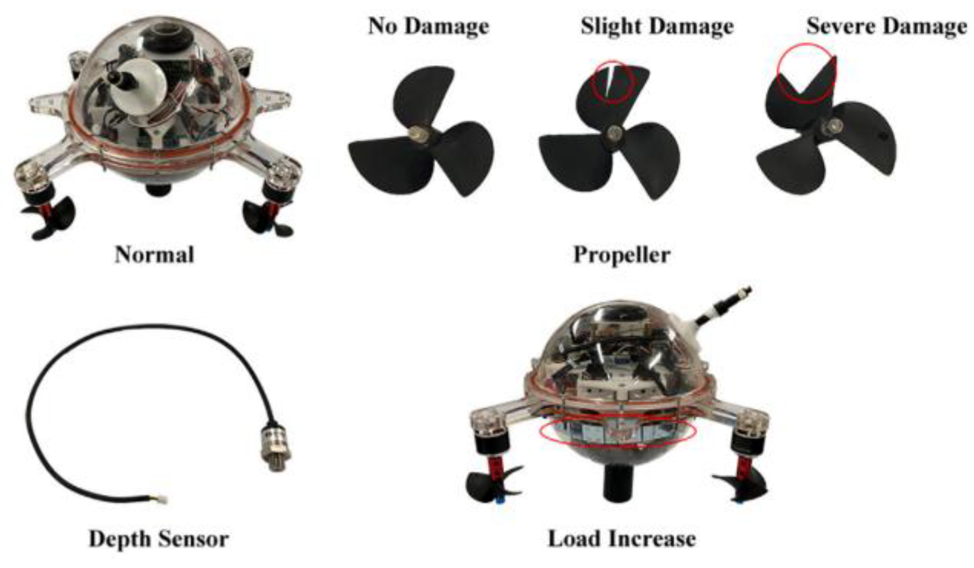
The dataset used in this paper for training and testing is available at https://data.mendeley.com/datasets/7rp2pmr6mx/1 (accessed on 1 June 2025), which is a complete open-source dataset. The experimental prototype for this dataset is a small AUV named “Haizhe”, independently developed by the Underwater Robot Laboratory of Zhejiang University. This AUV is lightweight and small in size, with main components including a motor, propeller, depth sensor, inertial measurement unit, central controller, and satellite positioning device. This dataset records five types of faults, including normal state, slight damage to the propeller, severe damage to the propeller, failure of the depth sensor, and load increase. The details of the fault settings are shown in Figure 5.

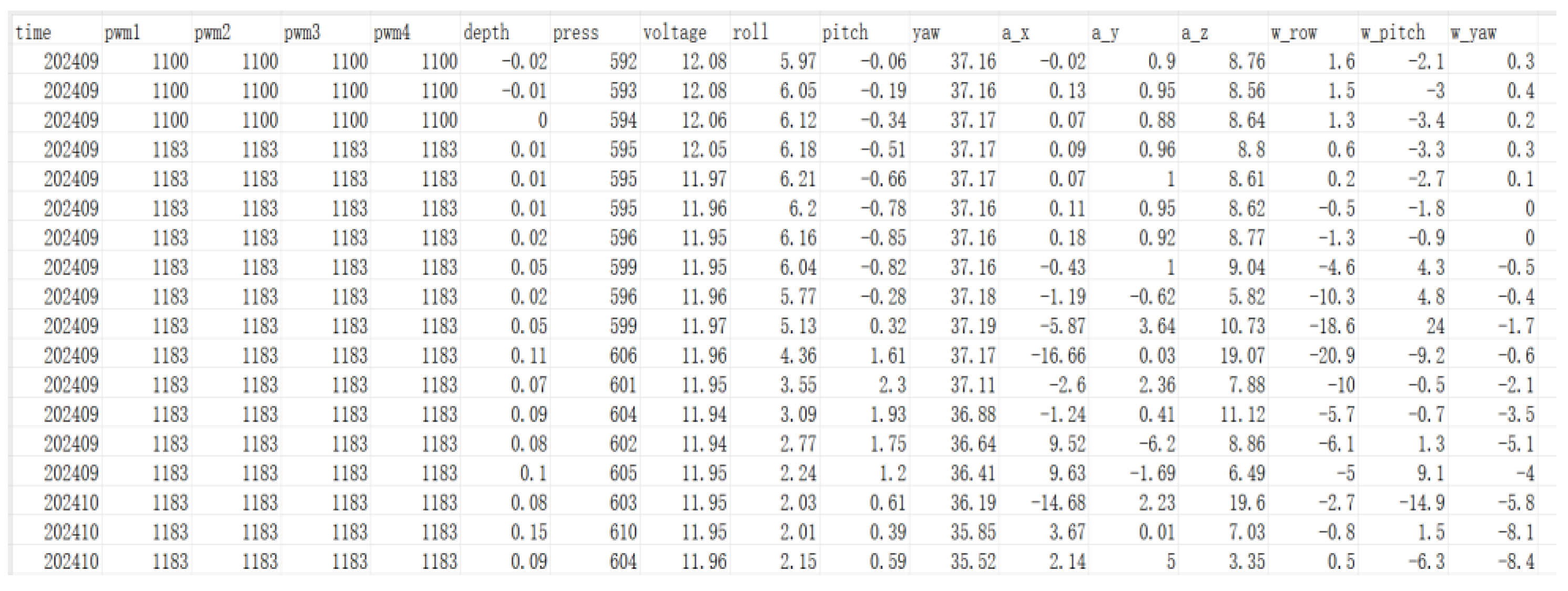
During each test, “Haizhe” executed the same program, operating underwater for 10–20 s per run. This ensured that the recorded state data was sufficiently lengthy to comprehensively reflect various indicators and their changing trends, serving as the data samples for further processing [31]. In the experiment, “Haizhe” had only one fault type at the same time, and there was no multi-failure concurrency. Each test recorded the navigation status data of the AUV and used it as a data sample, forming a real label with the corresponding fault type. This dataset has a large amount of data and authentic content, so this article is based on this dataset to complete the learning and evaluation of the fault diagnosis model, the statistical data of the dataset is shown in

Table 1. The statistical data of the dataset. Training: Training set size. Test: Test set size.

Fault State	Label	Dataset Size	Training	Test
Normal	0	182	146	36
AddWeight	1	268	214	54
PressureGain_constant	2	266	213	53
PropellerDamage_bad	3	249	199	50
PropellerDamage_slight	4	260	208	52

, A portion of the original dataset is shown in Figure 6.

3.2. Feature Extraction

The time series lengths of the training and testing datasets are different. In order to facilitate neural network processing, the time series length is set to 196. If the original sequence length is insufficient, the last row of data is used to fill in. If the original sequence length is too long, the excess part will be truncated. Each sample data in the original dataset contains 17 feature variables. Given that some feature variables contain no fault information, eight of them are selected to constitute the feature vectors for fault diagnosis learning and evaluation. Accordingly, the eigenvector can be expressed as: $\mathit{X}= \left[depth, press, roll, pitch, yaw, w\_row, w\_pitch, w\_yaw\right]$. The time series feature vectors used for training and testing are shown in Figure 7.

Accordingly, the training set comprises 980 samples, each being a 196 × 8 matrix, and the test set comprises 245 samples of the same size, with all samples corresponding to five distinct thruster states. For pattern recognition problems, the quality of feature vectors can greatly affect the performance of the model. In order to provide high-quality feature vectors to the diagnostic model, this paper adopts some data preprocessing operations.

3.2.1. Data Normalization

The feature vectors contain variables with different units of measurement. Consequently, data normalization is applied to eliminate scaling effects and unify the features onto a common scale. A widely used technique is Z-score normalization, which transforms the data to have a mean of 0 and a standard deviation of 1, approximating a standard normal distribution. This method accelerates model convergence and is simple to implement; nonetheless, it is highly sensitive to outliers. Given that AUV sensor readings in practical operations are often subject to missing or anomalous values, this study employs a robust normalization approach. This method replaces the mean and standard deviation in the Z-score calculation with robust statistical measures (e.g., median and interquartile range), thereby achieving a more stable and reliable scaling transformation. The specific steps are as follows:

(1)

Calculating the Median

Sort the eigenvalues within the eigenvector in ascending order, identify the two middle values, and compute their average, denoted as ${\mathit{X}}_{\mathit{m}\mathit{e}\mathit{d}\mathit{i}\mathit{a}\mathit{n}}$;

(2)

Clculating the Interquartile Range (IQR)

Sort the eigenvalues in the eigenvector from smallest to largest, and sequentially determine the first quartile ($Q_1$) and the third quartile ($Q_3$). The interquartile range is then calculated as:

$$IQR = Q_3 - Q_1$$

(1)

(3)

Performing Robust Normalization

Apply robust normalization to each raw data point X, yielding the following result:

$${\mathit{X}}_{\mathit{r}\mathit{o}\mathit{b}\mathit{u}\mathit{s}\mathit{t}} = {\displaystyle \frac{\mathit{X} - {\mathit{X}}_{\mathit{m}\mathit{e}\mathit{d}\mathit{i}\mathit{a}\mathit{n}}}{IQR}}$$

(2)

3.2.2. Missing Value Processing

Within AUV network control systems, online data missing due to transmission packet loss is random and non-systematic—its occurrence is unpredictable and follows no apparent pattern. The length of feature vectors should always be consistent, so when missing or invalid values appear in the dataset, they need to be filled in. For scenarios involving both univariate and multivariate missing data, the forward fill imputation or mean imputation method can be employed.

(1)

Forward fill imputation

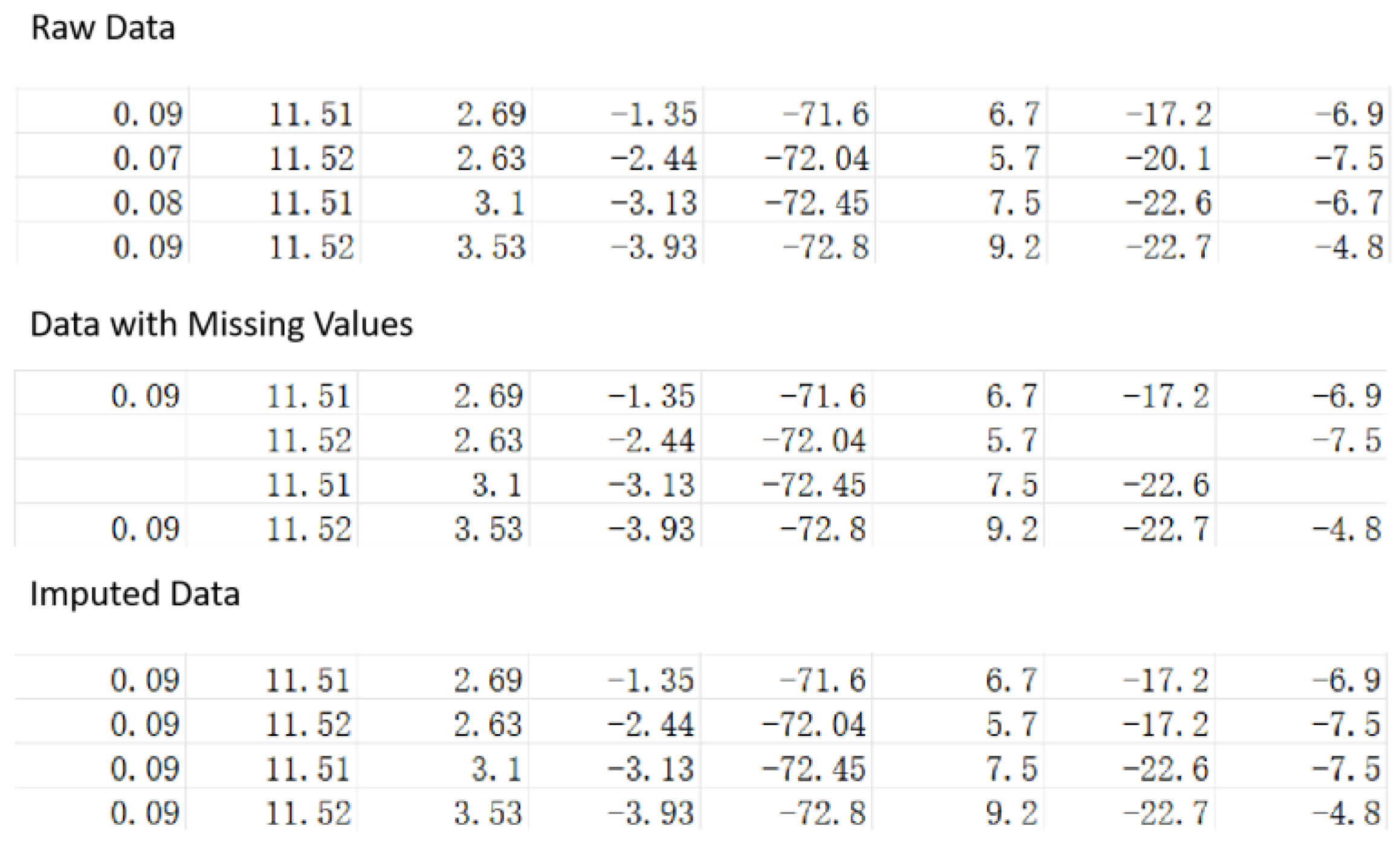
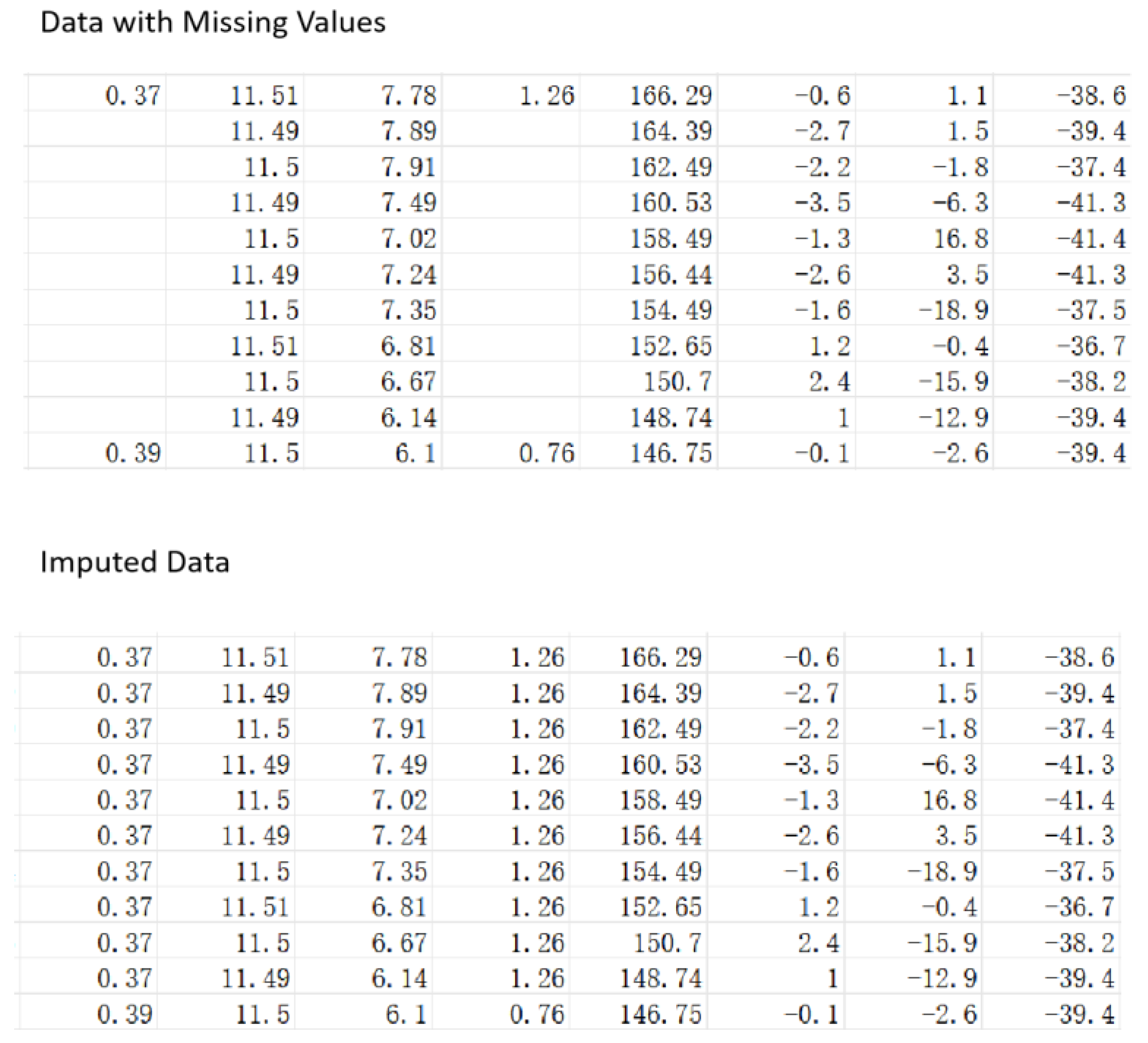
Forward fill imputation, often abbreviated as “ffill,” is a simple and commonly used method for handling missing data in sequential datasets, particularly time series. It operates under the assumption that the most recent valid observation is the best substitute for a missing value. For time series data, this means ordering the data points chronologically. The system scans the dataset sequentially, from the beginning to the end. As the scan progresses, each data point is checked for a valid value. When a missing value is encountered, the algorithm copies the last observed valid value and uses it to fill the gap. Missing data in random vectors can be either intermittent or consecutive; therefore, we have accounted for the impact of both scenarios on fault diagnosis. Figure 8 and Figure 9 illustrate examples of intermittent and continuous data missingness and their imputation, respectively.

(2)

Local mean imputation

For random missing patterns, the commonly used strategy is to fill in missing values with statistical indicators such as mean, median, etc. This article adopts the local mean imputation method to address the problem of random eigenvalue missing in the dataset, in order to ensure the integrity of the data. The local mean imputation method implemented in this study employs a temporally aware approach for handling missing values in multivariate time series data by calculating replacement values from the two preceding and two succeeding available observations within the same feature dimension. This neighborhood-based strategy preserves temporal continuity and local patterns while incorporating a hierarchical fallback mechanism that defaults to global feature means when local neighbors are unavailable, and ultimately to zero-imputation in cases of complete feature absence. The algorithm processes each feature dimension independently across all samples, maintaining the intrinsic temporal characteristics of sensor data while ensuring robustness across varying missingness patterns, making it particularly suitable for AUV monitoring applications where temporal correlations are strong and missing values frequently occur in contiguous blocks. The results of mean imputation are shown in Figure 10:

4. Model

LSTM is a special recursive neural network used for processing time series data, which can learn long-term dependency relationships and solve the gradient vanishing problem of RNN algorithms [32]. It performs well in long sequence tasks. Under the condition of single variable random missing, the original LSTM has high accuracy and fast learning speed. However, for the multivariate random missing condition, the accuracy of the original LSTM decreases rapidly. Therefore, this paper adopts an improved LSTM algorithm to solve the fault diagnosis problem under this condition.

4.1. LSTM

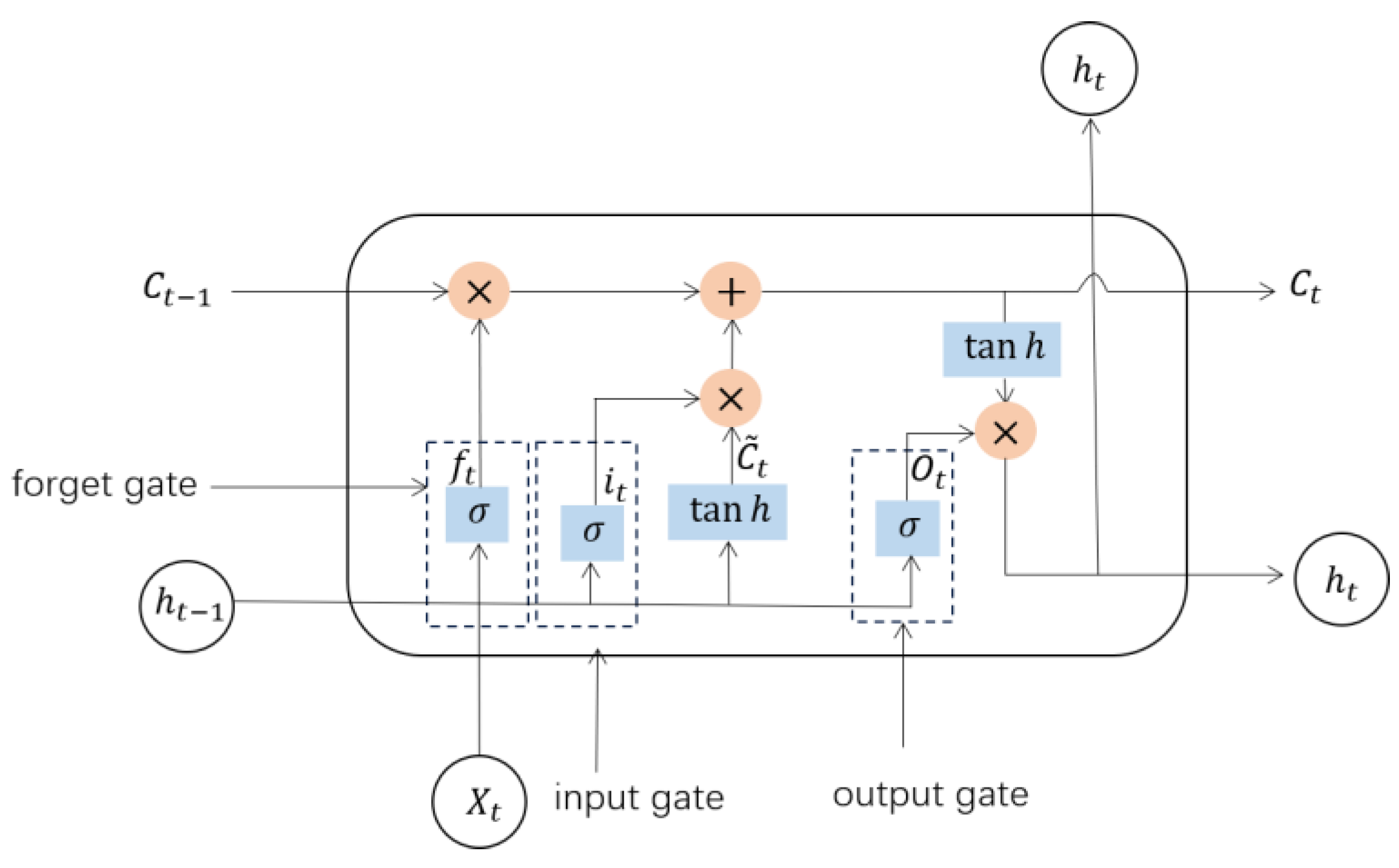
An LSTM unit consists of the following components: cell state, hidden state, forget gate, input gate, and output gate. LSTM controls the flow of information through a gating mechanism, determining which information should be remembered and which should be forgotten. The overall structure of LSTM cells is shown in Figure 11:

(1)

Forget gate

The forget gate determines the extent of information to be discarded from the previous cell state, with its calculation formula presented as follows:

$$f_t=\sigma \left(W_f·\left[h_{t-1},x_t\right]+b_f\right)$$

(3)

In the equation, $f_t$ is the output vector of the forget gate, which has the same dimension as the cell state dimension. The value of each element determines the corresponding position and degree of retention. $\sigma \left(·\right)$ represents the sigmoid activation function, with an output range of [0, 1], where 0 indicates complete forgetting and 1 indicates complete retention. $W_f$ is the weight matrix of the forget gate, $\left[h_{t-1},x_t\right]$ represents concatenating the previous hidden state with the current input, and $b_f$ is the bias of the forget gate.

(2)

Input gate

The input gate is used to control whether to incorporate the data at time $t$ into the control unit of the unit state. Firstly, extract effective information, and its calculation formula is as follows:

$${\tilde{C}}_t=tanh\left(W_c·\left[h_{t-1},x_t\right]+b_c\right)$$

(4)

In the formula, ${\tilde{C}}_t$ is the suggested updated value, which includes the new information at time $t$. $tanh\left(·\right)$ is a hyperbolic tangent function with an output range of [−1, 1]. $W_c$ and $b_c$ represent the weight matrix and bias, respectively. The calculation formula for the second output of the input gate is as follows:

$$i_t=\sigma \left(W_i·\left[h_{t-1},x_t\right]\right)+b_i$$

(5)

In the formula, $i_t$ is the output of the input gate, and $W_i$ and $b_i$ represent the weight matrix and bias, respectively. Update the cell state based on the outputs of the input gate and forget gate, using the following formula:

$$C_t=f_t\ast C_{t-1}+i_t\ast {\tilde{C}}_t$$

(6)

In the formula, $f_t\ast C_{t-1}$ represents forgetting some old information, and $i_t\ast {\tilde{C}}_t$ represents adding some new information.

(3)

Output gate

The output gate is a neural layer used by LSTM units to calculate the output value at time $t$. The output layer first extracts effective information from the integrated vector of the input value at time t and the output value at time $t - 1$. The output calculation formula of the output gate is as follows:

$$o_t=\sigma \left(W_o·\left[h_{t-1},x_t\right]+b_o\right)$$

(7)

In the formula, ${\sigma }_t$ represents the output of the output gate, $W_o$ and $b_o$ represent the weight matrix and bias, respectively. Based on the cell state at time $t$ and the output gate output, update the hidden state using the following formula:

$$h_t=o_t\ast tanh\left(C_t\right)$$

(8)

In the formula, $h_t$ represents the hidden state at time $t$, it is the final output at time t and also the input at time $t + 1$.

4.2. BiLSTM

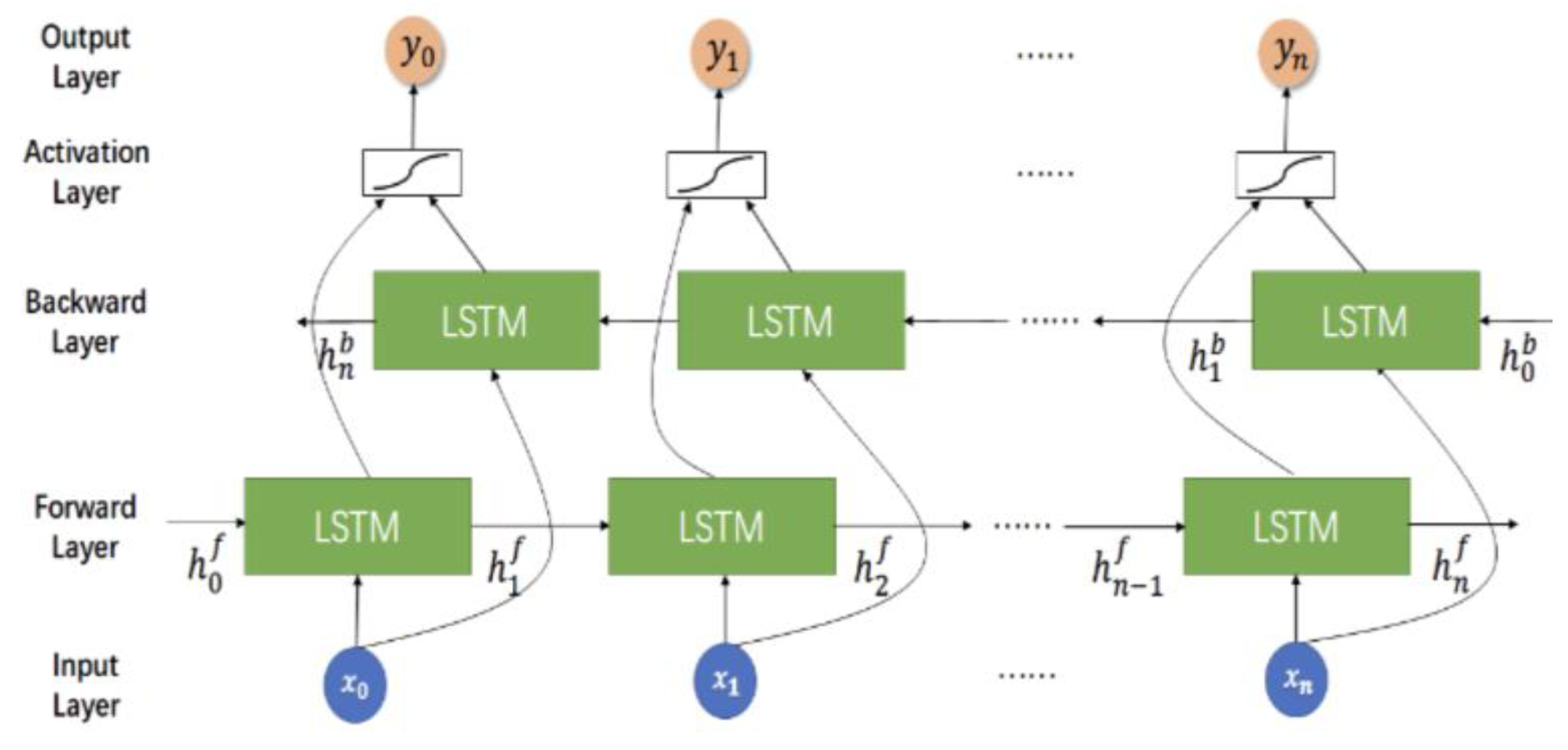
Conventional LSTMs process sequences strictly in a forward temporal direction, thereby limiting their contextual understanding to past information only. In contrast, Bidirectional LSTMs (BiLSTMs) address this constraint by employing two parallel LSTM layers—one processing the sequence in its original order and the other in reverse. This architecture enables the model to simultaneously incorporate both past and future context at each time step, allowing every output node to capture comprehensive information from the entire input sequence.

During the forward pass, the input sequence is fed sequentially into the first LSTM layer, and the hidden states at all time steps are computed and retained. Simultaneously, in the backward pass, the same input sequence is processed in reverse temporal order by the second LSTM layer, with its corresponding hidden states also being computed and stored. Finally, at each time step, the outputs from both directional layers are merged, typically via concatenation, to form the final contextualized representation. The architecture of the BiLSTM is illustrated in Figure 12.

4.3. Training

Common LSTMs are trained by minimizing cross-entropy loss on the training set, with parameters updated via the Adam algorithm. Let $\mathit{\Theta }$ denote all the trainable parameters of the model, the network can be trained by minimizing the following Cross-Entropy Loss with respect to $\mathit{\Theta }$:

$$\mathit{\Theta }=\underset{\Theta }{\arg \min }J\left(\mathit{\Theta }\right)$$

(9)

$$J\left(\mathit{\Theta }\right)={\displaystyle \sum }_{\left(x,y\right)\in \Omega }\left(-{\displaystyle \sum }_{i=1}^K{y}_i\log p_i\right)$$

(10)

$$y_i=\left\{\begin{array}{c}0, y\ne i\\ 1, y=i\end{array}\right.$$

(11)

$$p_i=p\left(i\left|x, \mathit{\Theta }\right.\right), {\displaystyle \sum }_{i=1}^K{p}_i=1$$

(12)

In the formula, $\mathit{\Theta }$ is the training set, $K$ is the number of labels, $x$ represents an input data, and $y$ represents the corresponding fault type. $p_i$ is a conditional probability which is computed from the model.

4.4. Modification

4.4.1. Improve the Loss Function

The conventional cross-entropy loss function quantifies the discrepancy between the predicted probability distribution generated by the LSTM model and the true label probability distribution. It propagates this discrepancy signal back to the LSTM through backpropagation, thereby guiding the model to adjust its weights and biases for improved accuracy. However, in AUV fault diagnosis tasks, different types of misclassification entail varying costs. For instance, misclassifying a “Severe damage to the propeller” as “normal state” may lead to the loss of the AUV, representing an extremely high cost, whereas misclassifying “normal state” as “failure of the depth sensor” may only trigger an unnecessary maintenance operation, resulting in a relatively low cost. Therefore, this paper designs a customized loss function to develop a risk-minimized AUV fault diagnosis model.

First, we define a 5 × 5 cost matrix C, where each element $C_{ij}$ represents the cost incurred when the true state is i, but the model predicts state j. The diagonal elements of the matrix are all set to 0, indicating that correct predictions incur zero cost. The off-diagonal elements are assigned positive values, with higher values indicating greater penalties for misclassification errors. Designing the cost matrix is not purely a mathematical task but rather a systems engineering problem that requires integrating domain knowledge, safety specifications, and mission requirements. As such, determining a completely accurate and unambiguous cost matrix is challenging. In this paper, the cost matrix is constructed by considering the impact of misclassification on both the safety of the AUV and the success of its mission. The cost matrix is shown in

Table 2. The cost matrix.

True Label Predicted Label	0	1	2	3	4
0	0	0	0	0	0
1	0.2	0	0	0	0
2	0.2	0	0	0	0
3	1.0	0	0	0	0
4	0.6	0	0	0	0

.

The values in the table can be modified according to the actual situation, and then define a loss function that considers the risk of misjudgment.

$$J_m\left(\mathit{\Theta }\right)=J\left(\mathit{\Theta }\right)+\lambda J_{cost}$$

(13)

In the formula, $J_m\left(\mathit{\Theta }\right)$ is the total loss of the model; $J\left(\mathit{\Theta }\right)$ is the Cross-Entropy Loss; $\lambda$ is used to adjust the importance of the regularization term, and $J_{cost}$ is the loss generated by the current diagnostic result.

4.4.2. Incorporate the Attention Mechanism

The Attention Mechanism is a method that mimics the human visual and cognitive systems, allowing neural networks to focus on relevant parts when processing input data. By incorporating the Attention Mechanism, neural networks can automatically learn and selectively focus on important information in the input, thereby improving the model’s performance and generalization ability. The global attention mechanism allows each element in the sequence to focus on all other elements, while the local attention mechanism limits the attention range of each element to a fixed local area.

This paper employs a temporal-aware feature attention mechanism. This mechanism comprises two critical branches: a temporal importance branch for capturing local temporal patterns, and a global importance branch for capturing holistic statistical characteristics. The workflow of the attention mechanism is illustrated in Figure 13.

(1)

Temporal Analysis

Firstly, A 1D convolution employs a sliding window across the time dimension for the feature extraction of local temporal patterns. Assuming 32 filters are used on the convolutional layer with a window size of 5, when the input sequence consists of 196 time steps and each time step contains 8 features, the convolutional layer will extract 32 different local patterns on each window of 5 consecutive time steps. Next, calculate the temporal importance, extract the maximum activation value of each filter, and map the importance of 32 temporal patterns onto 8 features.

(2)

Global Analysis

Calculate three global statistics, specifically the maximum value, mean, and standard deviation. The maximum value is important for anomaly detection, the mean represents the benchmark level of the feature, and the standard deviation reflects the volatility of the feature. Using a fully connected network to enable network learning of the most critical statistical information.

Linearly add the temporal importance and global importance, and then use the sigmoid function to limit the weights between [0, 1]. Attention weights are shared across all time steps, and each sample has its own unique feature importance pattern. To prevent gradient vanishing, the output of the attention layer will retain some of the original information to avoid excessive adjustment.

4.5. BiLSTM-Attention-MiniLoss

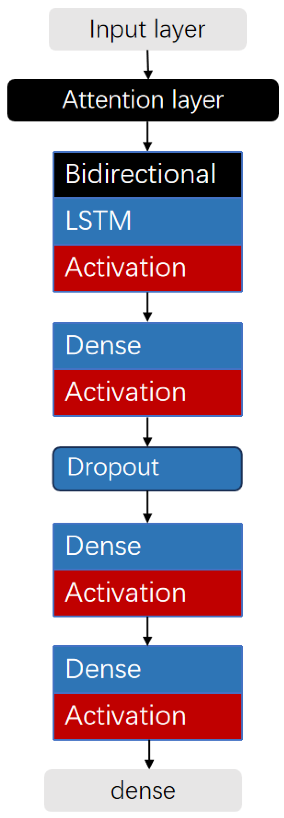
In general, the accuracy of the BiLSTM model is higher. Therefore, this paper uses the BiLSTM algorithm as the fault diagnosis base model, and adds an attention layer after the input layer of the model. To minimize the risk loss caused by the diagnostic results of the model, the minimum risk loss function is used to update the model weights. The BiLSTM model that integrates the attention mechanism and the minimum loss function is referred to as the BiLSTM-Attention-MiniLoss model. The structure of the AUV fault diagnosis model based on improved LSTM is shown in Figure 14:

5. Experiment

The experiment used the open-source deep learning library TensorFlow developed by the Google Brain team, and was performed on an Intel (R) Core (TM) i7-14650HX configuration CPU@2.20 (Intel, Santa Clara, CA, USA) Conduct experiments on a computer with GHz and 16 GB memory. Using the training and testing sets described in Table 1, a total of 980 training samples and 245 testing samples were included. Each sample is an 8-dimensional feature vector with a time series length of 196. These feature vectors were used to train and evaluate LSTM and improved models, respectively.

The number of trainable parameters of the LSTM and BiLSTM models is presented in

Table 3. The number of trainable parameters for LSTM.

Layer Model	LSTM
LSTM layer (128 units)	4 × (8 × 128 + 128 × 128 + 128) = 70,144
Dense layer (64 units)	128 × 64 + 64 = 8256
Dense layer (32 units)	64 × 32 + 32 = 2080
Dense layer (5 units)	32 × 5 + 5 = 165

and

Table 4. The number of trainable parameters for BiLSTM.

Layer Model	BiLSTM
BiLSTM layer (128 units)	2 × [4 × (8 × 128 + 128 × 128 + 128)] = 140,288
Dense layer (64 units)	128 × 64 + 64 = 8256
Dense layer (32 units)	64 × 32 + 32 = 2080
Dense layer (5 units)	32 × 5 + 5 = 165

Compared with the BiLSTM model, the BiLSTM-Attention-MiniLoss model incorporates an attention layer, and the number of trainable parameters of the attention layer is provided in

Table 5. The number of trainable parameters for Attention.

Layer Model	Attention
Conv1D (32 filters)	(5 × 8 + 1) × 32 = 1312
Temporal weight	32 × 8 = 256
Global weight	24 × 2 + 2 = 50
Global weight	2 × 8 + 8 = 24

.

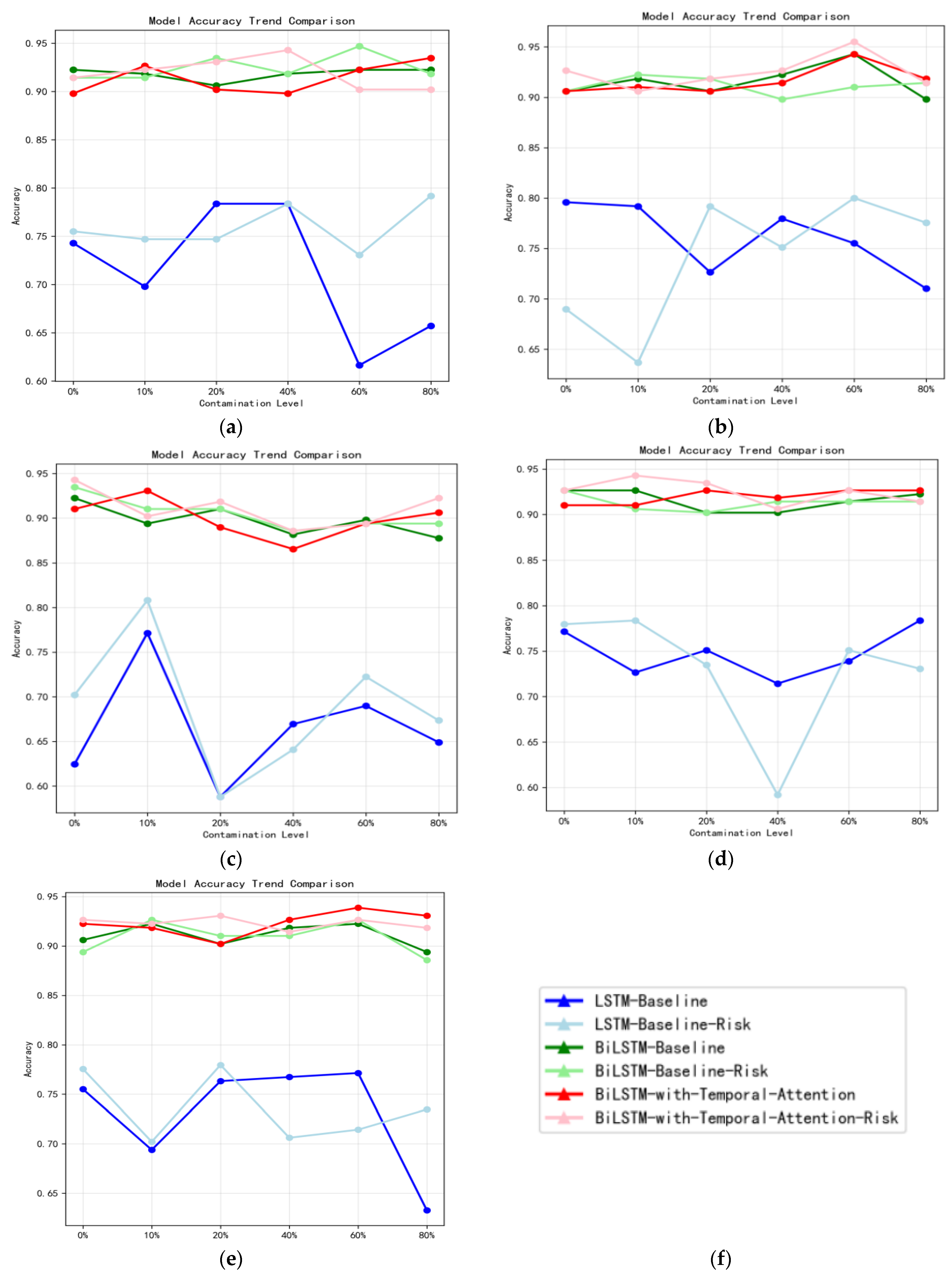
Based on the aforementioned dataset and model, we completed multiple sets of experiments. For both univariate missing and multivariate missing conditions, a comparative analysis of fault diagnosis performance between LSTM and BiLSTM-Attention-MiniLoss was conducted under missing rates of 0%, 10%, 20%, 40%, 60%, and 80%. The average accuracy of the diagnostic model under different working conditions is shown in

Table 6. The average accuracy of the diagnostic model under different working conditions. a: intermittent univariate missing data, forward fill imputation; b: intermittent multivariate missing data, forward fill imputation; c: continuous multivariate missing data, forward fill imputation; d: intermittent univariate missing data, local mean imputation; e: intermittent multivariate missing data, local mean imputation.

Working Conditions	LSTM-CE	LSTM-MiniLoss	BiLSTM-CE	BiLSTM-MiniLoss	BiLSTM-Attention_CE	BiLSTM-Attention-MiniLoss
a	0.7136	0.7592	0.9184	0.9245	0.9136	0.9190
b	0.7632	0.7407	0.9157	0.9116	0.9163	0.9245
c	0.6653	0.6891	0.8973	0.8998	0.8993	0.9109
d	0.7476	0.7286	0.9156	0.9129	0.9197	0.9252
e	0.7306	0.7354	0.9109	0.9088	0.9231	0.9231

. Under different missing rates in the scenario of continuous multivariate missing data, the detailed losses and average losses of each model using forward interpolation imputation are shown in

Table 7. The loss of the diagnostic model under different missing rate.

Missing Rate	LSTM-CE	LSTM-MiniLoss	BiLSTM-CE	BiLSTM-MiniLoss	BiLSTM-Attention_CE	BiLSTM-Attention-MiniLoss
0%	0.9970	0.7929	0.2393	0.2053	0.2355	0.2250
10%	0.6147	0.5437	0.2966	0.2553	0.2158	0.2906
20%	1.0649	1.0766	0.2485	0.2720	0.2689	0.2249
40%	0.9564	0.9793	0.3818	0.3066	0.3762	0.2899
60%	0.7268	0.7219	0.2671	0.3058	0.2418	0.3020
80%	0.8831	0.8011	0.3068	0.3201	0.2504	0.2465
Mean loss	0.8738	0.8193	0.2900	0.2775	0.2648	0.2632

. The comparative experimental accuracy results are presented in Figure 15 and Figure 16.

As can be seen from Table 6, the proposed BiLSTM-Attention-MiniLoss model demonstrates superior performance across multiple experimental sets. Table 7 shows the loss values when the model employs forward imputation under the scenario of continuous multivariate missing data. In this experiment, the BiLSTM-Attention-MiniLoss model achieved an accuracy increase of 36.9% and a loss reduction of 69.89% compared to the original LSTM model; when compared to the BiLSTM model, it improved accuracy by 1.5% and reduced loss by 9.3%. It can be observed that the BiLSTM-Attention-MiniLoss model achieves the smallest loss. However, the difference in losses between the model using cross-entropy loss and the one using minimum risk loss is marginal, which is primarily attributable to an overly conservative design of the cost matrix. While we are currently unable to provide a more rational cost matrix and can only empirically set its values to demonstrate the necessity of incorporating risk considerations, a more accurate update of the cost matrix will be pursued in future work.

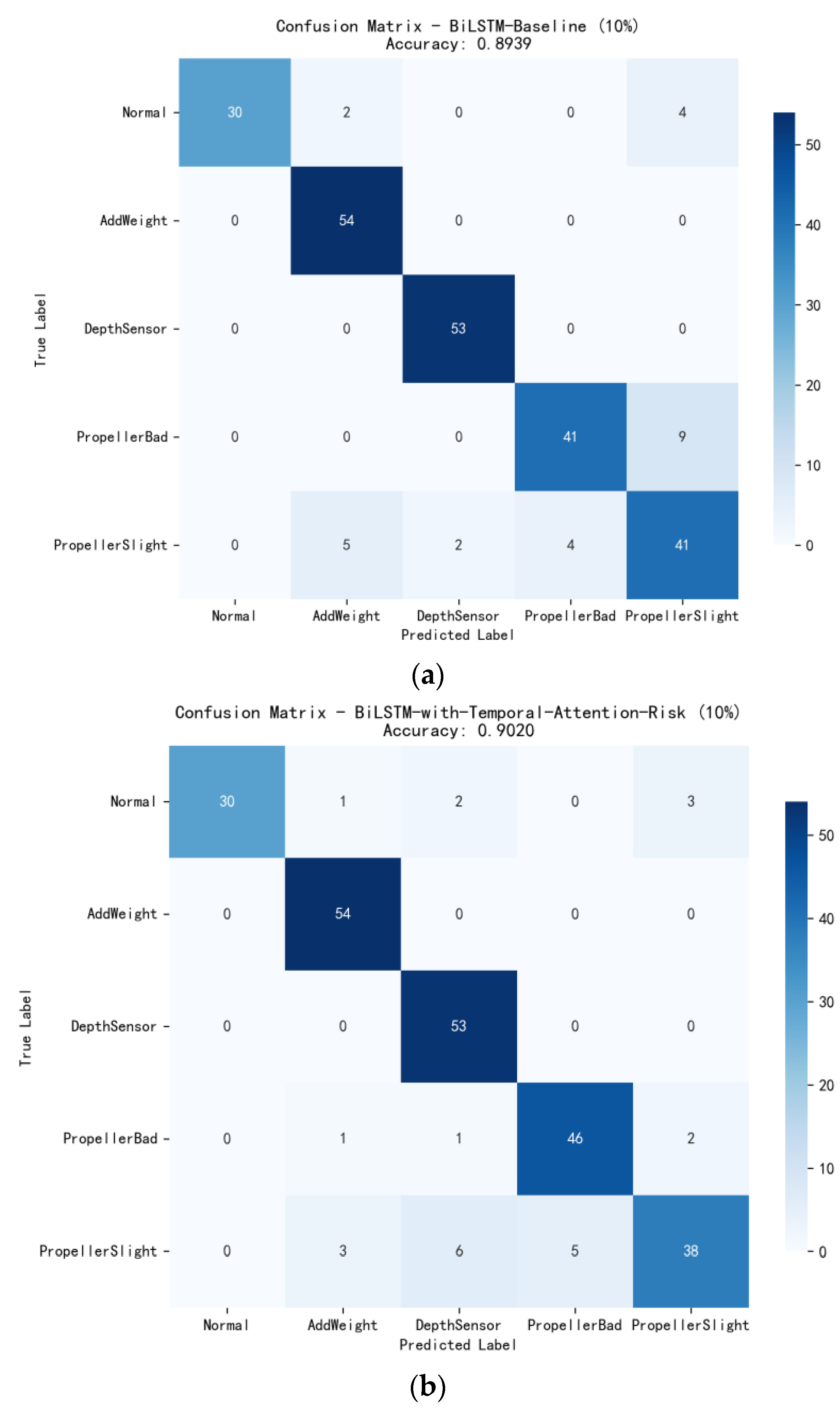
Figure 15 presents the detailed accuracy of each model under various data missing rates across the five experimental sets. Under a 10% continuous data missing rate with forward fill imputation, Figure 16 presents a comparison of the confusion matrices between the BiLSTM and BiLSTM-Attention-MiniLoss models. The confusion matrices allow for a detailed observation of the number of correctly and incorrectly classified samples.

The experimental results indicate that the original LSTM exhibits significant fluctuations in accuracy as the data missing rate increases, whereas the BiLSTM-Attention-MiniLoss model demonstrates much smaller variations, reflecting its stronger robustness. Furthermore, after incorporating the attention mechanism and the minimum risk loss function, the original BiLSTM shows improved accuracy and reduced loss.

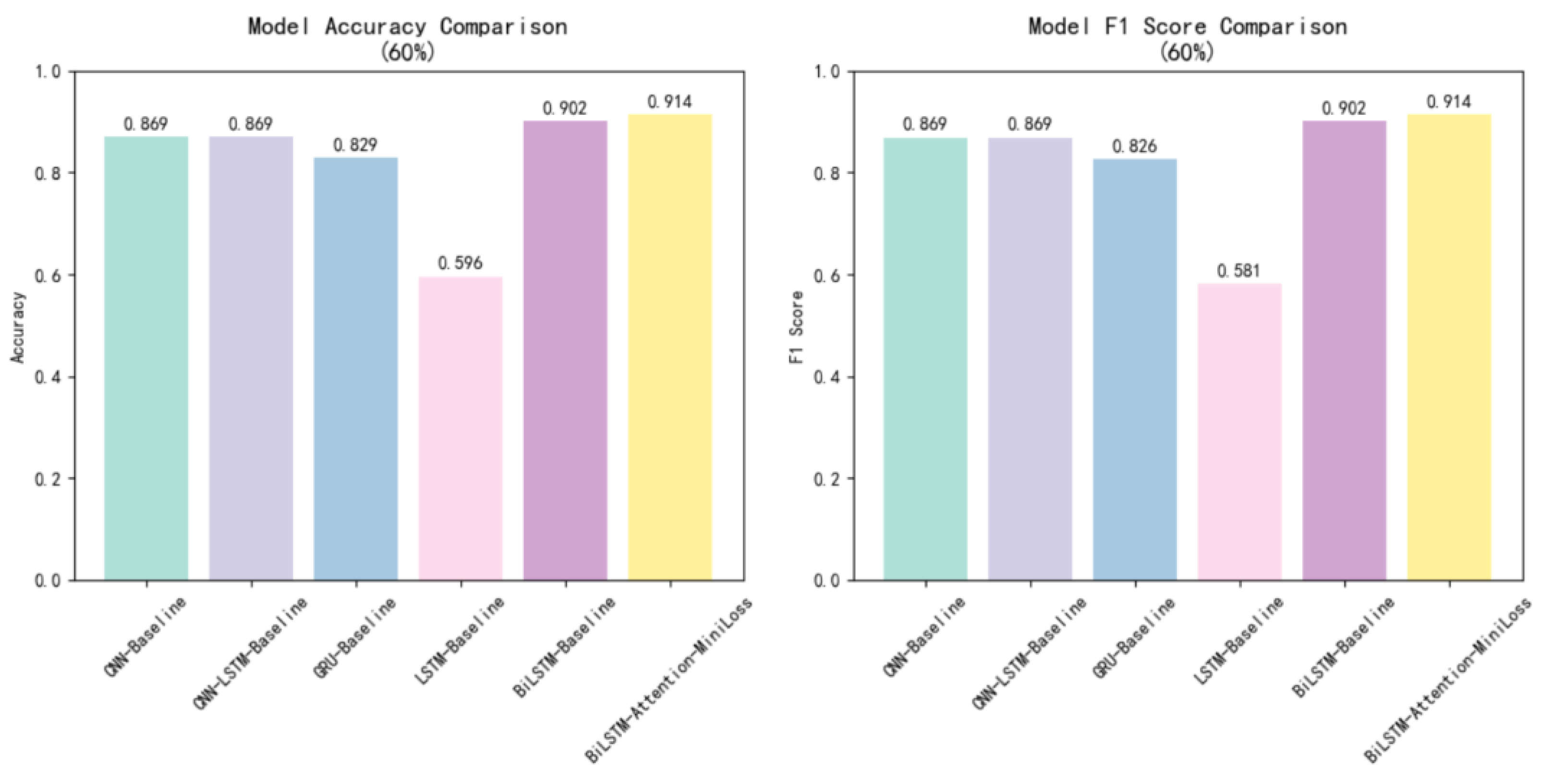
To demonstrate the effectiveness of the proposed model, we conducted comparative experiments with diagnostic models. Under continuous multivariate missing data conditions using forward-filling imputation, the accuracy comparison results of different models are shown in Figure 17. The experimental results indicate that the proposed model exhibits relatively superior performance.

6. Conclusions

A model-free fault diagnosis scheme with a new diagnosis algorithm BiLSTM-Attention-MiniLoss was proposed in this paper. The improved model incorporates a temporal-aware feature attention mechanism, which directs the model’s focus to more critical parts of the input by computing attention weights at the feature level. These weights are determined with full consideration of the temporal context. Additionally, to account for the varying costs associated with different types of misclassification, the improved model adopts a minimum risk-based loss function. Experimental results demonstrate that the incorporation of the attention mechanism and the minimum risk loss function into the BiLSTM model leads to an increase in accuracy and a reduction in loss.

Future Work Directions: Enable the fault diagnosis model to possess lifelong learning capabilities, equipping it with the ability to learn new fault types. The current method is only capable of handling single-fault diagnosis; future efforts will focus on enhancing the model to achieve multiple-fault diagnosis. Given the potential for more complex data missingness or noise in the dataset, it is imperative to propose more effective data preprocessing methods. A more rational update of the cost matrix will be pursued in future work.

References

1. Li, T.; Hou, S.; Li, D. Overview and research progress of fault identification method. Prog. Geophys. 2018, 33, 1507–1514. [Google Scholar]
2. Zhang, M.; Liu, C.; Wang, Y.; Chen, T. Fault Diagnosis for Autonomous Underwater Vehicles Using a Combined Model-Based and Data-Driven Approach. IEEE J. Ocean. Eng. 2021, 46, 987–1001. [Google Scholar]
3. Li, Y.; Zhao, W.; Zhang, J. Actuator Fault Diagnosis and Fault-Tolerant Control for Autonomous Underwater Vehicles. Ocean Eng. 2019, 172, 37–46. [Google Scholar]
4. Huang, J.; Zhang, M.; Wang, S. A Review of Fault Diagnosis and Fault-Tolerant Control for Autonomous Underwater Vehicles. Annu. Rev. Control. 2018, 45, 42–54. [Google Scholar]
5. Wang, Y.; Zhang, Q.; He, B. Sensor Fault Diagnosis and Reconstruction for Autonomous Underwater Vehicles Based on Deep Learning. IEEE Sens. J. 2022, 22, 15231–15242. [Google Scholar]
6. Zhang, T.; Li, X.; Zhang, Y. Fault Detection and Isolation for Autonomous Underwater Vehicles Using Sliding Mode Observers. Int. J. Adapt. Control Signal Process. 2017, 31, 735–751. [Google Scholar]
7. Ranganathan, N.; Patel, M.I.; Sathyamurthy, R. An intelligent system for failure detection and control in an autonomous underwater vehicle. IEEE Trans. Syst. Man Cybern.-Part A Syst. Hum. 2001, 31, 762–767. [Google Scholar] [CrossRef]
8. Hamilton, K.; Lane, D.M.; Brown, K.E.; Evans, J.; Taylor, N.K. An integrated diagnostic architecture for autonomous underwater vehicles. J. Field Robot. 2007, 24, 497–526. [Google Scholar] [CrossRef]
9. Zheng, Y.; Wang, G.; Chen, Z.; Liu, Y.; Shen, X. A finite state machine based diagnostic expert system of large-scale autonomous unmanned submarine. In Proceedings of the 2018 IEEE 8th International Conference on Underwater System Technology: Theory and Applications (USYS), Wuhan, China, 1–8 December 2018; IEEE: Piscataway, NJ, USA, 2018; pp. 1–6. [Google Scholar]
10. Miguelanez, E.; Patron, P.; Brown, K.E.; Petillot, Y.R.; Lane, D.M. Semantic knowledge-based framework to improve the situation awareness of autonomous underwater vehicles. IEEE Trans. Knowl. Data Eng. 2010, 23, 759–773. [Google Scholar] [CrossRef]
11. Alireza, M.; Zhang, Y.; Zhang, J. A hybrid fault diagnosis framework for autonomous underwater vehicles: Enhancing rule-based systems with neural networks. Ocean Eng. 2021, 235, 109357. [Google Scholar]
12. Xu, D.; Jiang, B.; Shi, P. A hybrid fault diagnosis methodology for autonomous underwater vehicles based on fuzzy logic and partial least squares. Int. J. Adapt. Control Signal Process. 2017, 31, 394–409. [Google Scholar]
13. Wang, Y.; Gao, Z.; Zhang, Q. Data-driven fault diagnosis for AUVs: Addressing the challenges of expert knowledge dependency and multiple faults. In Proceedings of the 2019 IEEE International Conference on Robotics and Automation (ICRA), Montreal, QC, Canada, 20–24 May 2019; IEEE: Piscataway, NJ, USA, 2019; pp. 6123–6129. [Google Scholar]
14. Ji, D.; Yao, X.; Li, S.; Tang, Y.; Tian, Y. Model-free fault diagnosis for autonomous underwater vehicles using sequence Convolutional Neural Network. Ocean Eng. 2021, 232, 108874. [Google Scholar] [CrossRef]
15. Shumsky, A.; Zhirabok, A.; Hajiyev, C. Observer based fault diagnosis in thrusters of autonomous underwater vehicle. In Proceedings of the 2010 Conference on Control and Fault-Tolerant Systems (SysTol), Nice, France, 6–8 October 2010; IEEE: Piscataway, NJ, USA, 2010; pp. 11–16. [Google Scholar]
16. Chu, Z.; Chen, Y.; Zhu, D.; Zhang, M. Observer-based fault detection for magnetic coupling underwater thrusters with applications in jiaolong HOV. Ocean Eng. 2020, 210, 107570. [Google Scholar] [CrossRef]
17. Jiang, C.; Lv, J.; Liu, Y.; Wang, G.; Xu, X.; Deng, Y. STF-based diagnosis of AUV thruster faults. In E3S Web of Conferences; EDP Sciences: Shenyang, China, 2022; Volume 360, p. 01048. [Google Scholar]
18. Li, Z.; Sun, J.; Zhang, W.; Du, J.; Hu, X. Modeling and controller design for underactuated AUVs in the presence of unknown ocean currents. Ocean Eng. 2023, 285, 115367. [Google Scholar]
19. Wang, Y.; Liu, J.; Zhang, M.; Du, J.; Li, Z. A robust fault diagnosis scheme for autonomous underwater vehicles with sensor faults under ocean current disturbances. Ocean Eng. 2022, 266, 113107. [Google Scholar]
20. Lei, Y.; Yang, B.; Jiang, X.; Jia, F.; Li, N.; Nandi, A.K. Applications of machine learning to machine fault diagnosis: A review and roadmap. Mech. Syst. Signal Process. 2020, 138, 106587. [Google Scholar] [CrossRef]
21. Liu, Q.; Zhu, D.; Yang, S.X. Unmanned underwater vehicles fault identification and fault-tolerant control method based on FCA-CMAC neural networks, applied on an actuated vehicle. J. Intell. Robot. Syst. 2012, 66, 463–475. [Google Scholar] [CrossRef]
22. Zhang, M.; Wu, J.; Chu, Z. Multi-fault diagnosis for autonomous underwater vehicle based on fuzzy weighted support vector domain description. China Ocean Eng. 2014, 28, 599–616. [Google Scholar] [CrossRef]
23. Nascimento, S.; Valdenegro-Toro, M. Modeling and soft-fault diagnosis of underwater thrusters with recurrent neural networks. Int. Fed. Autom. Control-Pap. 2018, 51, 80–85. [Google Scholar] [CrossRef]
24. Jiang, Y.; He, B.; Lv, P.; Guo, J.; Wan, J.; Feng, C.; Yu, F. Actuator fault diagnosis in autonomous underwater vehicle based on principal component analysis. In Proceedings of the 2019 IEEE Underwater Technology (UT), Kaohsiung, Taiwan, 16–19 April 2019; IEEE: Piscataway, NJ, USA, 2019; pp. 1–5. [Google Scholar]
25. Xia, S.; Zhou, X.; Shi, H.; Li, S.; Xu, C. A fault diagnosis method with multi-source data fusion based on hierarchical attention for AUV. Ocean Eng. 2022, 266, 112595. [Google Scholar] [CrossRef]
26. Li, Y.; Ye, Y.; Zhang, Z.; Wen, L. A New Incremental Learning Method Based on Rainbow Memory for Fault Diagnosis of AUV. Sensors 2025, 25, 4539. [Google Scholar] [CrossRef]
27. Zhang, S.; Ye, F.; Wang, B.; Zhang, J.; Han, Y.; Chang, H. A deep transfer learning based data-driven method for ship energy system fault diagnosis. Ocean Eng. 2023, 285, 115353. [Google Scholar]
28. Wang, J.; Liang, Y.; Zheng, Y.; Zhang, A.; Liu, Z. A deep learning-based method for bearing fault diagnosis with anti-strong noise and variable load capability. Measurement 2020, 165, 108100. [Google Scholar]
29. Mai, J.; Huang, H.; Wei, F.; Yang, C.; He, W. Autonomous underwater vehicle fault diagnosis model based on a deep belief rule with attribute reliability. Ocean Eng. 2025, 321, 120472. [Google Scholar] [CrossRef]
30. Mai, J.; Luo, Z.; Ge, G.; Zhang, G.; He, W. A Fault Diagnosis Method for Autonomous Underwater Vehicles Based on Online Extended Belief Rule Base with Dynamic Rule Reduction. IEEE Access 2024, 12, 165407–165424. [Google Scholar] [CrossRef]
31. Ji, D.; Yao, X.; Li, S.; Tang, Y.; Tian, Y. Autonomous underwater vehicle fault diagnosis dataset. Data Brief 2021, 39, 107477. [Google Scholar] [CrossRef] [PubMed]
32. Huo, Y.; Gang, S.; Guan, C. FCIHMRT: Feature Cross-Layer Interaction Hybrid Method Based on Res2Net and Transformer for Remote Sensing Scene Classification. Electronics 2023, 12, 4362. [Google Scholar] [CrossRef]
Figure 1. Fault diagnosis process based on rule.
Applsci 15 11570 g001
Figure 2. Fault diagnosis process based on model.
Applsci 15 11570 g002
Figure 3. Fault diagnosis process based on a data-driven approach.
Applsci 15 11570 g003
Figure 4. Flowchart of the diagnosis process.
Applsci 15 11570 g004
Figure 5. Fault types setting for ‘Haizhe’. The red circles indicate the fault locations.
Applsci 15 11570 g005
Figure 6. A subset of the raw data.
Applsci 15 11570 g006
Figure 7. Schematic diagram of time series feature vectors.
Applsci 15 11570 g007
Figure 8. Intermittent Data Missingness and Imputation Results.
Applsci 15 11570 g008
Figure 9. Continuous Data Missingness and Imputation Results.
Applsci 15 11570 g009
Figure 10. The results of mean imputation.
Applsci 15 11570 g010
Figure 11. The overall structure of an LSTM cell.
Applsci 15 11570 g011
Figure 12. The architecture of the BiLSTM.
Applsci 15 11570 g012
Figure 13. The workshop of the proposed attention mechanism.
Applsci 15 11570 g013
Figure 14. The structure of fault diagnosis model for AUV.
Applsci 15 11570 g014
Figure 15. Comparison of Accuracy of Each Model Under Various Data Missing Rates. (a) intermittent univariate missing data, forward fill imputation; (b) intermittent multivariate missing data, forward fill imputation; (c) continuous multivariate missing data, forward fill imputation; (d) intermittent univariate missing data, local mean imputation. (e) intermittent multivariate missing data, local mean imputation. (f) The description of line types.
Applsci 15 11570 g015
Figure 16. Comparison of Confusion Matrix. (a) BiLSTM; (b) BiLSTM-Attention-MiniLoss.
Applsci 15 11570 g016
Figure 17. Comparison of Diagnostic Model Accuracy.
Applsci 15 11570 g017